Article

A Generalization of the Bivariate Gamma Distribution Based on Generalized Hypergeometric Functions

by
Christian Caamaño-Carrillo
1 and
Javier E. Contreras-Reyes
2,*
1
Departamento de Estadística, Facultad de Ciencias, Universidad del Bío-Bío, Concepción 4081112, Chile
2
Instituto de Estadística, Facultad de Ciencias, Universidad de Valparaíso, Valparaíso 2360102, Chile
*
Author to whom correspondence should be addressed.
Mathematics 2022, 10(9), 1502; https://doi.org/10.3390/math10091502
Submission received: 20 March 2022 / Revised: 26 April 2022 / Accepted: 28 April 2022 / Published: 1 May 2022
(This article belongs to the Special Issue Probability, Statistics and Their Applications 2021)

Abstract

:
In this paper, we provide a new bivariate distribution obtained from a Kibble-type bivariate gamma distribution. The stochastic representation was obtained by the sum of a Kibble-type bivariate random vector and a bivariate random vector builded by two independent gamma random variables. In addition, the resulting bivariate density considers an infinite series of products of two confluent hypergeometric functions. In particular, we derive the probability and cumulative distribution functions, the moment generation and characteristic functions, the Hazard, Bonferroni and Lorenz functions, and an approximation for the differential entropy and mutual information index. Numerical examples showed the behavior of exact and approximated expressions.

1. Introduction

Let Z i k , i = 1 , , ν , ν > 2 , an independent sequence of standardized normal random variables with correlation C o r r ( Z i k , Z i k ) = ρ , i j , and let U k = i = 1 ν Z i k 2 with k = 1 , 2 , then U k is a random variable with χ ν 2 marginal distribution. According to [1], the distribution of U = ( U 1 , U 2 ) has a correlated bivariate chi-square distribution with ν degrees of freedom parameter and probability density function (pdf) given by
f U ( u ) = 2 ν ( u 1 u 2 ) ( ν 2 ) / 2 e ( u 1 + u 2 ) 2 ( 1 ρ 2 ) Γ 2 ν 2 ( 1 ρ 2 ) ν / 2 F 0 , 1 ν 2 ; ρ 2 u 1 u 2 4 ( 1 ρ 2 ) 2 ,
where F p , q ( a 1 , a 2 , , a p ; b 1 , b 2 , , b p ; x ) denotes the generalized hypergeometric function defined by
F p , q ( a 1 , a 2 , , a p ; b 1 , b 2 , , b q ; x ) = k = 0 ( a 1 ) k ( a 2 ) k ( a p ) k ( b 1 ) k ( b 2 ) k ( b q ) k x k k ! ,
for p , q = 0 , 1 , 2 , , and with ( a ) k = Γ ( k + a ) Γ ( a ) , k N { 0 } , being the Pochhammer symbol [2]. Note that in this case, the correlation function of U is given by ρ U = ρ 2 .
Transformation W = U β , β > 0 defines a random variable G a m m a ( ν / 2 , β / 2 ) distributed with density
f W ( w ) = β 2 ν / 2 w ν / 2 1 Γ ν 2 e β 2 w , w > 0 .
The pdf of W = ( W 1 , W 2 ) has a Kibble-type correlated bivariate gamma distribution [3], given by
f W ( w ) = 2 ν β ν ( w 1 w 2 ) ν / 2 1 e β 2 ( 1 ρ 2 ) ( w 1 + w 2 ) Γ ν 2 2 ( 1 ρ 2 ) ν / 2 F 0 , 1 ν 2 ; β 2 ρ 2 w 1 w 2 4 ( 1 ρ 2 ) 2 ,
where E ( W ) = ν β , V a r ( W ) = 2 ν β 2 and ρ W = ρ 2 . In Equations (1) and (4), the case ρ = 0 implies the product of two independent chi-square and gamma random variables (i.e., the same result obtained by the bivariate normal distribution in the independency case).
The univariate and bivariate gamma distributions are basic distributions that have been used to model data in many applications [4,5]. More recently, several examples of bivariate distributions and their applications emerged: streamflow data [6], drought data modeling [7], rainfall data modeling [8], wind speed data spatio-temporal modeling [9], flood volume-peak data modeling [10], wireless communications models [11], and transmit antennas system modeling [12].
In this paper, we build a generalization of bivariate gamma distribution using a Kibble type bivariate gamma distribution. The stochastic representation was obtained by the sum of a Kibble-type bivariate random vector and a bivariate random vector builded by two independent gamma random variables. In addition, the resulting bivariate density considers an infinite series of products of two confluent hypergeometric functions. In particular, we derive the pdf and cumulative distribution function (cdf), moment generation and characteristic functions, Hazard, Bonferroni and Lorenz functions, and an approximation for the differential entropy and mutual information index. Numerical examples showed the behavior of exact and approximated expressions. All numerical examples were calculated using the hypergeo package of R software [13].
The paper is organized as follows. Section 2 presents the generalization of the bivariate gamma distribution, with its pdf (with simulations), cdf, moment generation and characteristic functions, cross-product moment, covariance and correlation (with simulations), and some special expected values. Moreover, the Hazard, Bonferroni and Lorenz functions are computed. Section 3 presents the approximation for the differential entropy and mutual information index (with simulations) for the generalized bivariate gamma distribution with some numerical results. The paper ends with a discussion in Section 4. Proofs are available in Appendix A section.

2. Bivariate Gamma Generalization

Let
Y = W + R ,
where R is a random variable, R G a m m a ( α / 2 , β / 2 ) , α > 0 and the distribution of W is defined by Equation (3); thus Y G a m m a ( ( α + ν ) / 2 , β / 2 ) is a random variable with marginal gamma distribution and arbitrary shape, ( α + ν ) / 2 , and scale, β / 2 , based on α , β and ν parameters. This type of construction has been proposed by [5,6,14,15,16,17,18,19] to build a bivariate gamma distribution. Specifically, the authors considered the case W 1 = W 2 in (3). Properties of the bivariate gamma distribution can be found in [15,18,20,21].
In line with the stochastic representation (5), we consider the bivariate distribution of Y = ( Y 1 , Y 2 ) as a generalization of the Cheriyan distribution [15], where
Y 1 = W 1 + R 1 , Y 2 = W 2 + R 2 ,
W = ( W 1 , W 2 ) is given in (3) and (4) with ρ W = ρ 2 , and R i G a m m a ( α i / 2 , β / 2 ) , α i > 0 , R i R j , i j , R i W j , i , j . Thus, Y G a m m a ( ( α k + ν ) / 2 , β / 2 ) , k = 1 , 2 .
In the following theorem, we provide a new bivariate distribution with gamma marginal distributions obtained using a Kibble-type bivariate gamma distribution [3].
Theorem 1.
Let W k = i = 1 ν Z i k 2 / β where Z i k , i = 1 , , ν , k = 1 , 2 , is a finite sequence of independent normal random variables with zero mean, unit variance, and correlation ρ. Let Y = W + R , with W = ( W 1 , W 2 ) and R k G a m m a ( α k / 2 , β / 2 ) , k = 1 , 2 . The pdf of Y = ( Y 1 , Y 2 ) is given by
f Y ( y ) = β 2 ν + α 1 + α 2 2 y 1 ( ν + α 1 ) / 2 1 y 2 ( ν + α 2 ) / 2 1 e β 2 ( 1 ρ 2 ) ( y 1 + y 2 ) Γ ν + α 1 2 Γ ν + α 2 2 ( 1 ρ 2 ) ν / 2 k = 0 ν 2 k k ! ν + α 1 2 k ν + α 2 2 k β 2 ρ 2 y 1 y 2 4 ( 1 ρ 2 ) 2 k × F 1 , 1 α 1 2 ; ν + α 1 2 + k ; β ρ 2 y 1 2 ( 1 ρ 2 ) F 1 , 1 α 2 2 ; ν + α 2 2 + k ; β ρ 2 y 2 2 ( 1 ρ 2 ) ,
where F 1 , 1 a 1 ; b 1 ; x is the confluent hypergeometric function defined in (2) for p = q = 1 .
Theorem 1 shows that the pdf considers an infinite series of products of two confluent hypergeometric functions. Note that when ρ = 0 , pdf in Theorem 1 becomes the product of two independent gamma random variables, G a m m a ( ( ν + α k ) / 2 , β / 2 ) , k = 1 , 2 , i.e., the same property of the bivariate normal distribution is accomplished. When α 1 = α 2 = 0 , then f Y ( y ) = f W ( w ) , i.e., Y is Kibble-type gamma distributed (see Figure 1).
Figure 1 shows the pdf of Equation (6) for some parameters of Y . When ρ increases, is produced the largest values of y 1 and y 2 in the pdf. When ρ = 0.25 , the pdf is close at origin ( y 1 , y 2 0 ), has positive bias and decays exponentially. When ρ = 0.5 , the pdf has less bias, but more symmetry and variability. When ρ = 0.75 , the pdf has a bias to the right, but with less bias than in the case ρ = 0.25 . When β increases (decreases), its variance increases (decreases). When ν increases, the pdf shows heavy-tailed behavior, at the same time as parameter α k , k = 1 , 2 increases (as the usual gamma distribution).
Theorem 2.
The joint cdf of Y = ( Y 1 , Y 2 ) in Equation (6) can be expressed as
F Y ( Y 1 t 1 , Y 2 t 2 ) = ( 1 ρ 2 ) ν + α 1 + α 2 2 k = 0 ν 2 k ρ 2 k k ! γ 2 , 1 α 1 2 , ν + α 1 2 + k , β t 1 2 ( 1 ρ 2 ) ; ν + α 1 2 + k ; ρ 2 × γ 2 , 1 α 2 2 , ν + α 2 2 + k , β t 2 2 ( 1 ρ 2 ) ; ν + α 2 2 + k ; ρ 2 ,
where γ 2 , 1 ( a 1 , ( a 2 , x ) ; b 1 ; z ) denotes the incomplete gaussian hypergeometric function as
γ 2 , 1 ( a 1 , ( a 2 , x ) ; b 1 ; z ) = k = 0 ( a 1 ) k ( a 2 ; x ) k ( b 1 ) k z k k ! ,
with incomplete Pochhammer symbols given by ( a 2 ; x ) k = γ ( a 2 + k , x ) Γ ( a 2 ) for a 2 , k C , x 0 [2,22].
Theorem 2 shows that the joint pdf considers an infinite series of products of two incomplete gaussian hypergeometric functions.

2.1. Moment Generation Function

In this section, we analyze the moment generation function of Y = ( Y 1 , Y 2 ) , the cross-product moment between Y 1 and Y 2 , and some particular expected values involving these variables.
Proposition 1.
The joint moment generation (mgf) and characteristic functions of Y = ( Y 1 , Y 2 ) given in Equation (6) are
M ( t 1 , t 2 ) = β ν / 2 β ( 1 ρ 2 ) [ β 2 ( 1 ρ 2 ) t 1 ] [ β 2 ( 1 ρ 2 ) t 2 ] β 2 ρ 2 ν 2 β ( 1 ρ 2 ) ( β 2 ( 1 ρ 2 ) t 1 ) β ρ 2 α 1 2 β ( 1 ρ 2 ) ( β 2 ( 1 ρ 2 ) t 2 ) β ρ 2 α 2 2
and
ϕ ( t 1 , t 2 ) = β ν / 2 β ( 1 ρ 2 ) [ β 2 ( 1 ρ 2 ) i t 1 ] [ β 2 ( 1 ρ 2 ) i t 2 ] β 2 ρ 2 ν 2 β ( 1 ρ 2 ) ( β 2 ( 1 ρ 2 ) i t 1 ) β ρ 2 α 1 2 β ( 1 ρ 2 ) ( β 2 ( 1 ρ 2 ) i t 2 ) β ρ 2 α 2 2 ,
respectively.
Assuming ρ = 0 , thus M ( t 1 , 0 ) = β β 2 t 1 ν + α 1 2 and M ( 0 , t 2 ) = β β 2 t 2 ν + α 2 2 , which are the mgf’s of a gamma random variable. The proof of the characteristic function of Y is trivial, following the proof of Proposition 1 for M ( t 1 , t 2 ) .
Proposition 2.
The cross-product moment of Y = ( Y 1 , Y 2 ) in Equation (6) can be expressed as
E ( Y 1 a Y 2 b ) = 2 β a + b ( 1 ρ 2 ) ( ν + α 1 + α 2 ) / 2 + a + b Γ ν + α 1 2 + a Γ ν + α 2 2 + b Γ ν + α 1 2 Γ ν + α 2 2 k = 0 ν 2 k ν + α 1 2 + a k ν + α 2 2 + b k k ! ν + α 1 2 k ν + α 2 2 k ρ 2 k × F 2 , 1 α 1 2 , ν + α 1 2 + a + k ; ν + α 1 2 + k ; ρ 2 F 2 , 1 α 2 2 , ν + α 2 2 + b + k ; ν + α 2 2 + k ; ρ 2 ,
where F 2 , 1 a 1 , a 2 ; b 1 ; x is the gaussian hypergeometric function defined in (2) for p = 2 and q = 1 .
Proposition 2 shows that the cross-product moment considers an infinite series of products of two gaussian hypergeometric functions. A direct result of Proposition 2 is the following Corollary 1, that presents the expected value and variance of marginal gamma random variable Y i , and the covariance and correlation between two marginal gamma random variables, Y 1 and Y 2 .
Corollary 1.
If Y = ( Y 1 , Y 2 ) , it has pdf according to (6). According to Proposition 2, we have
 (a) 
E ( Y k ) = ν + α k β , k = 1 , 2 .
 (b) 
V a r ( Y k ) = 2 ( ν + α k ) β 2 , k = 1 , 2 .
 (c) 
C o v ( Y 1 , Y 2 ) = ( ν + α 1 ) ( ν + α 2 ) β 2 [ ( 1 ρ 2 ) ν / 2 k = 0 ν 2 k ν + α 1 2 + 1 k ν + α 2 2 + 1 k k ! ν + α 1 2 k ν + α 2 2 k ρ 2 k × 1 ρ 2 ν + 2 k ν + α 1 + 2 k 1 ρ 2 ν + 2 k ν + α 2 + 2 k 1 ] .
 (d) 
ρ Y = ( ν + α 1 ) ( ν + α 2 ) 2 [ ( 1 ρ 2 ) ν / 2 k = 0 ν 2 k ν + α 1 2 + 1 k ν + α 2 2 + 1 k k ! ν + α 1 2 k ν + α 2 2 k ρ 2 k × 1 ρ 2 ν + 2 k ν + α 1 + 2 k 1 ρ 2 ν + 2 k ν + α 2 + 2 k 1 ] .
The proofs of parts (a) and (b) are trivial. For parts (c) and (d), the Euler formula (9.131.1.11) of [23] is used, F 2 , 1 ( a , b , c , ; x ) = ( 1 x ) c b a F 2 , 1 ( c a , c b , c ; x ) , and Proposition 2 with a = b = 1 .
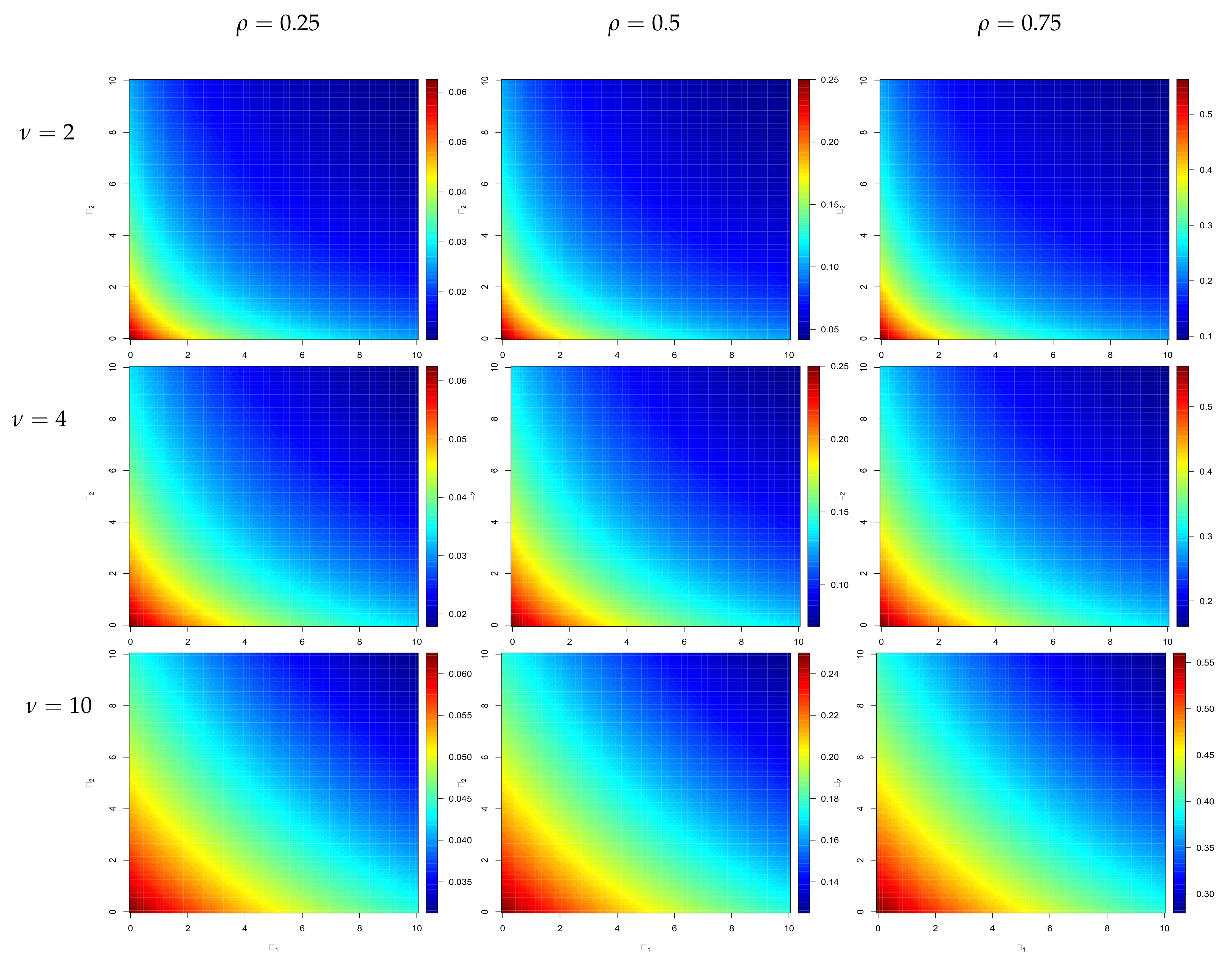
Figure 2 shows the correlation ρ Y of Corollary 1d for some pdf parameters of Y (6). For all cases, when α 1 and α 2 increase, the correlation ρ Y decreases. When ν increases, correlation ρ Y slowly decreases from small to large values of α 1 and α 2 . When parameter ρ (the normal distribution correlation) increases, the correlation ρ Y increases, as does its maximum value (from 0.06 to 0.55). We can observe in Corollary 1d that correlation ρ Y does not depend on β .
The following Proposition 3 is useful for computing differential entropy and mutual information index of Section 3.
Proposition 3.
If Y = ( Y 1 , Y 2 ) have pdf given in (6), then
 (a) 
E Y [ Y i ] = 2 ( 1 ρ 2 ) ( ν + α i ) / 2 + 1 Γ ν + α i 2 + 1 β Γ ν + α i 2 k = 0 ν 2 k ν + α i 2 + 1 k ρ 2 k k ! ν + α i 2 k F 2 , 1 α i 2 , ν + α i 2 + 1 + k ; ν + α i 2 + k ; ρ 2 ,
        i , j = 1 , 2 , i j .
 (b) 
E Y [ log Y i ] = ( 1 ρ 2 ) ( ν + α i ) / 2 k = 0 m 1 = 0 ν 2 k α i 2 m 1 ρ 2 ( k + m 1 ) k ! m 1 ! ψ ν + α i 2 + k + m 1 log β 2 ( 1 ρ 2 ) , if ρ > 0 ; ψ ν + α i 2 log β 2 , if ρ = 0 .
        i , j = 1 , 2 , i j ; where ψ ( x ) = d d x log Γ ( x ) is the digamma function.

2.2. Hazard, Bonferroni and Lorenz Functions

The Bonferroni and Lorenz curves [24] have many practical applications not only in economy, but also in fields like reliability, lifetime testing, insurance, and medicine. For random vector Y = ( Y 1 , Y 2 ) with cdf F ( y ) = F Y ( Y 1 y 1 , Y 2 y 2 ) , the Hazard, Bonferroni and Lorenz functions are defined by
Z Y ( t ) = f Y ( t ) 1 F ( t ) ,
with t = ( t 1 , t 2 ) ;
B q ( Y ) = 1 F ( y ) E [ Y ] 0 q 0 q y f Y ( y ) d y 1 d y 2 ,
with q a real scalar, 0 < q < + ; and
L q ( Y ) = B q ( y ) E [ Y ] ,
respectively.
The Bonferroni curve for pdf (6) considered F ( y ) and E [ Y ] , obtained from Theorem 2 and Proposition 2 (by replacing a = b = 1 ), respectively. The double integral of the left side of (14) is obtained with the following Proposition.
Proposition 4.
Let Y = ( Y 1 , Y 2 ) be a random vector with pdf given in (6) and q a real scalar, 0 < q < + , thus
0 q 0 q y f Y ( y ) d y 1 d y 2 = 4 ( 1 ρ 2 ) ( ν + α 1 + α 2 ) / 2 + 2 Γ ν + α 1 2 + 1 Γ ν + α 2 2 + 1 β 2 Γ ν + α 1 2 Γ ν + α 2 2 × k = 0 ν 2 k ν + α 1 2 + 1 ν + α 2 2 + 1 ρ 2 k k ! ν + α 1 2 ν + α 2 2 × γ 2 , 1 α 1 2 , ν + α 1 2 + 1 + k , β q 2 ( 1 ρ 2 ) ; ν + α 1 2 + k ; ρ 2 × γ 2 , 1 α 2 2 , ν + α 2 2 + 1 + k , β q 2 ( 1 ρ 2 ) ; ν + α 2 2 + k ; ρ 2 ,
where γ 2 , 1 ( a 1 , ( a 2 , x ) ; b 1 ; z ) is denoted in Theorem 2.
Given that F ( y ) and E [ Y ] depend on incomplete and complete gaussian hypergeometric functions, respectively, the Hazard, Bonferroni and Lorenz curves can be computed using these functions.

3. Differential Entropy and Mutual Information Index

The differential entropy of a random variable Y is a variation measure of information uncertainty [25]. In particular, the differential entropy of Y = ( Y 1 , Y 2 ) with pdf f Y ( y ) is defined by
H ( Y ) = E Y [ log { f Y ( Y ) } ] = 0 0 f Y ( y ) log f Y ( y ) d y 1 d y 2 ,
and measures the contained information in Y based on its pdf’s parameters. The following Remarks 1 and 2 will be used in the Proposition 5 to approximate the differential entropy of Y .
Remark 1 
([26]). For a positive and fixed y i , and fixed parameters α k , k = 1 , 2 , ρ and β, we have
F 1 , 1 α i 2 ; ν + α i 2 ; β ρ 2 y i 2 ( 1 ρ 2 ) = s = 0 n 1 ( α i 2 ) s ( ν + α i 2 ) s s ! β ρ 2 y 2 2 ( 1 ρ 2 ) s + O ( | ν | n ) , n = 1 , 2 , ,
as | ν | .
Remark 2.
(Formula 1.511 of [23]). If n and x = u / n (i.e., x turn around 0, 1 < x 1 , and there exists a constant μ > 0 such that | log ( 1 + u / n ) u / n | μ / n 2 ) , see Lemma 3.2 of [27]), we get
log ( 1 + x ) = x + O ( n 2 ) .
Proposition 5.
The differential entropy of a random vector Y = ( Y 1 , Y 2 ) with probability density function given in (6) can be approximated as
H ( Y ) log β 2 ν + α 1 + α 2 2 ( 1 ρ 2 ) ν / 2 Γ ν + α 1 2 Γ ν + α 2 2 ν + α 1 2 1 E Y [ log Y 1 ] ν + α 2 2 1 E Y [ log Y 2 ] β 2 ( 1 ρ 2 ) ρ 2 ( α 1 2 ) 1 ( ν + α 1 2 ) 1 1 E Y [ Y 1 ] + ρ 2 ( α 2 2 ) 1 ( ν + α 2 2 ) 1 1 E Y [ Y 2 ] ,
where E Y [ Y k ] and E Y [ log Y k ] , k = 1 , 2 , can be computed using parts (a) and (b) of Proposition 3, respectively.
Under dependence assumption ( ρ 0 ), the mutual information index (MII) [25,28,29] between Y 1 and Y 2 is defined by
M ( Y 1 , Y 2 ) = E log f Y ( y 1 , y 2 ) f Y 1 ( y 1 ) f Y 2 ( y 2 ) = 0 0 f Y ( y 1 , y 2 ) log f Y ( y 1 , y 2 ) f Y 1 ( y 1 ) f Y 2 ( y 2 ) d y 1 d y 2 .
It is clear from (17) that MII between Y 1 and Y 2 can be expressed in terms of marginal and joint differential entropies, M ( Y ) = H ( Y 1 ) + H ( Y 2 ) H ( Y ) [25]. According to (5), the differential entropy of each gamma distribution is
H ( Y k ) = α k + ν 2 log β 2 + log Γ α k + ν 2 + 1 α k + ν 2 ψ α k + ν 2 , k = 1 , 2 .
Therefore, the MII between Y 1 and Y 2 can be computed using (18) and Proposition (5). Under independence assumption ρ = 0 , the mutual information index between Y 1 and Y 2 is 0; otherwise, this index is positive [28,29]. Moreover, the MII increases with the degree of dependence between the components of Y 1 and Y 2 . Therefore, the MII is an association measure between Y 1 and Y 2 , which could be compared with correlation ρ Y .
Figure 3 illustrates the behavior of MII assuming several values for parameters of Y . The case ρ = 0 was omitted for the above mentioned reasons, and the case ρ = 0.5 was omitted because results are similar to the case ρ = 0.25 . We observed that M ( Y 1 , Y 2 ) < 0 for small values of β , which is related to approximation (A16) being wrongly utilized when the argument is outside ( 1 , 1 ] in Remark 2. However, when the argument is inside ( 1 , 1 ] , we get M ( Y 1 , Y 2 ) > 0 and increases for large values of β and any values of ν , as in the analysis of ρ Y in Figure 2.

4. Concluding Remarks

In this paper, we presented a generalization of bivariate gamma distribution based on a Kibble type bivariate gamma distribution. The stochastic representation was obtained by the sum of a Kibble-type bivariate random vector and a bivariate random vector builded by two independent gamma random variables. Moreover, the resulting bivariate density considers an infinite series of products of two confluent hypergeometric functions. In particular, we derived the probability and cumulative distribution functions, moment generation and characteristic functions, covariance, correlation and cross-product moment, Hazard, Bonferroni and Lorenz functions, and an approximation for the differential entropy and mutual information index. Numerical examples showed the behavior of exact and approximated expressions.
Previous work by [30] considered the generalization of this paper to represent bivariate Superstatistics based on Boltzmann factors. However, further work derived from this study could extend to the multivariate case (d-dimensional). A possible extension is considering Equation (6) of [31] for the joint pdf of our vector ( W 1 , , W d ) , corresponding to a pdf based on a gamma distribution with simple Markov chain-type correlation. When d = 2 , this pdf coincides with Kibble distribution defined in (4). Thus,
Y 1 = W 1 + R 1 Y d = W d + R d ,
where R 1 , , R d , R i G a m m a ( α i / 2 , β / 2 ) , i = 1 , , d are independent and gamma distributed random variables. However, the properties obtained in this study could be difficult to obtain for this multivariate version and the use of generalized hypergeometric function must be carefully handled. In addition, it is possible to consider the Probability Transformation method using the theory of the space transformation of random variables and the probability conservation principle. Thus, we could evaluate the pdf of a d-dimensional invertible transformation [32].
Inferential aspects could also be considered in future work. For example: (i) a numerical approach could be used in the optimization of log-likelihood function; (ii) the pseudo-likelihood method by considering the optimization of an objective function that depends on a bivariate pdf could be used; and (iii) a Bayesian approach could be useful.

Author Contributions

C.C.-C. and J.E.C.-R. wrote the paper and contributed reagents/analysis/ materials tools; C.C.-C. and J.E.C.-R. conceived, designed and performed the experiments. All authors have read and approved the final manuscript.

Funding

Caamaño-Carrillo’s research was funded by FONDECYT (Chile) grant No. 11220066 and by Proyecto Regular DIUBB 2120538 IF/R de la Universidad del Bío-Bío. Contreras-Reyes’s research was funded by FONDECYT (Chile) grant No. 11190116.

Institutional Review Board Statement

Not applicable.

Informed Consent Statement

Not applicable.

Data Availability Statement

Not applicable.

Acknowledgments

The authors thank the editor and three anonymous referees for their helpful comments and suggestions.

Conflicts of Interest

The authors declare that there is no conflict of interest in the publication of this paper.

Appendix A

Proof of Theorem 1. 
Let w 1 = y 1 r 1 and w 2 = y 2 r 2 be a transformation in (4), 0 < r k < y k , k = 1 , 2 , with Jacobian J ( ( w 1 , w 2 ) ( y 1 , y 2 ) ) = 1 . Using series expansion of the hypergeometric function F 0 , 1 , we get
f Y ( y ) = 0 y 1 0 y 2 f W | R ( w | r ) f R ( r ) | J | d r = 0 y 1 0 y 2 β 2 ν + α 1 + α 2 2 [ ( y 1 r 1 ) ( y 2 r 2 ) ] ν / 2 1 r 1 α 1 / 2 1 r 2 α 2 / 2 1 e β 2 ( 1 ρ 2 ) [ ( y 1 r 1 ) + ( y 2 r 2 ) ] e β 2 ( r 1 + r 2 ) Γ 2 ν 2 Γ α 1 2 Γ α 2 2 ( 1 ρ 2 ) ν / 2 × F 0 , 1 ν 2 ; β 2 ρ 2 ( y 1 r 1 ) ( y 2 r 2 ) 4 ( 1 ρ 2 ) 2 d r = k = 0 0 y 1 0 y 2 β 2 ν + α 1 + α 2 2 [ ( y 1 r 1 ) ( y 2 r 2 ) ] ν / 2 + k 1 r 1 α 1 / 2 1 r 2 α 2 / 2 1 e β 2 ( 1 ρ 2 ) ( y 1 + y 2 ) e β ρ 2 2 ( 1 ρ 2 ) ( r 1 + r 2 ) Γ 2 ν 2 Γ 2 α 2 ( 1 ρ 2 ) ν / 2 × 1 k ! ν 2 k β 2 ρ 2 4 ( 1 ρ 2 ) 2 k d r = β 2 ν + α 1 + α 2 2 e β 2 ( 1 ρ 2 ) ( y 1 + y 2 ) Γ 2 ν 2 Γ α 1 2 Γ α 2 2 ( 1 ρ 2 ) ν / 2 k = 0 I ( k ) k ! ν 2 k β 2 ρ 2 4 ( 1 ρ 2 ) 2 k .
Then, using Fubini’s Theorem and formula (3.383.1.11) of [23], we obtain
I ( k ) = 0 y 1 ( y 1 r 1 ) ν / 2 + k 1 r 1 α 1 / 2 1 e β ρ 2 2 ( 1 ρ 2 ) r 1 d r 1 0 y 2 ( y 2 r 2 ) ν / 2 + k 1 r 2 α 2 / 2 1 e β ρ 2 2 ( 1 ρ 2 ) r 2 d r 2 = Γ 2 ν 2 + k Γ α 1 2 Γ α 2 2 Γ ν + α 1 2 + k Γ ν + α 2 2 + k y 1 ( ν + α 1 ) 2 + k 1 y 2 ( ν + α 2 ) 2 + k 1 F 1 , 1 α 1 2 ; ν + α 1 2 + k ; β ρ 2 y 1 2 ( 1 ρ 2 ) × F 1 , 1 α 2 2 ; ν + α 2 2 + k ; β ρ 2 y 2 2 ( 1 ρ 2 ) .
Combining Equations (A2) and (A1), the result is obtained. □
Proof of Theorem 2.
Using series expansion of the hypergeometric function F 1 , 1 , we get
F Y ( Y 1 t 1 , Y 2 t 2 ) = 0 t 1 0 t 2 f Y ( y ) d y = β 2 ν + α 1 + α 2 2 Γ ν + α 1 2 Γ ν + α 2 2 ( 1 ρ 2 ) ν / 2 0 t 1 0 t 2 y 1 ( ν + α 1 ) / 2 1 y 2 ( ν + α 2 ) / 2 1 e β 2 ( 1 ρ 2 ) ( y 1 + y 2 ) × k = 0 ν 2 k k ! ν + α 1 2 k ν + α 2 2 k β 2 ρ 2 y 1 y 2 4 ( 1 ρ 2 ) 2 k F 1 , 1 α 1 2 ; ν + α 1 2 + k ; β ρ 2 y 1 2 ( 1 ρ 2 ) × F 1 , 1 α 2 2 ; ν + α 2 2 + k ; β ρ 2 y 2 2 ( 1 ρ 2 ) d y = β 2 ν + α 1 + α 2 2 Γ ν + α 1 2 Γ ν + α 2 2 ( 1 ρ 2 ) ν / 2 k = 0 m 1 = 0 m 2 = 0 ν 2 k I ( k , m 1 , m 2 ) k ! ν + α 1 2 k ν + α 2 2 k β 2 ρ 2 4 ( 1 ρ 2 ) 2 k × α 1 2 m 1 m 1 ! ν + α 1 2 + k m 1 β ρ 2 2 ( 1 ρ 2 ) m 1 α 2 2 m 2 m 2 ! ν + α 2 2 + k m 2 β ρ 2 2 ( 1 ρ 2 ) m 2 .
Using Fubini’s Theorem and formula (3.381.1) of [23], we obtain
I ( k , m 1 , m 2 ) = 0 t 1 y 1 ( ν + α 1 ) / 2 + k + m 1 1 e β y 1 2 ( 1 ρ 2 ) d y 1 0 t 1 y 2 ( ν + α 2 ) / 2 + k + m 2 1 e β y 2 2 ( 1 ρ 2 ) d y 2 = 2 ( 1 ρ 2 ) β ( ν + α 1 ) / 2 + k + m 1 2 ( 1 ρ 2 ) β ( ν + α 2 ) / 2 + k + m 2 × γ ν + α 1 2 + k + m 1 , β t 1 2 ( 1 ρ 2 ) γ ν + α 2 2 + k + m 2 , β t 2 2 ( 1 ρ 2 ) ,
where γ ( a , x ) = x e t t a 1 d t , a > 0 is the lower incomplete gamma function. Combining Equations (A3) and (A4), we obtain
F Y ( Y 1 t 1 , Y 2 t 2 ) = ( 1 ρ 2 ) ( ν + α 1 + α 2 ) / 2 Γ ν + α 1 2 Γ ν + α 2 2 k = 0 ν 2 k ρ 2 k k ! ν + α 1 2 k ν + α 2 2 k × m 1 = 0 α 1 2 m 1 γ ν + α 1 2 + k + m 1 , β t 1 2 ( 1 ρ 2 ) ρ 2 m 1 m 1 ! ν + α 1 2 + k m 1 m 2 = 0 α 2 2 m 2 γ ν + α 2 2 + k + m 2 , β t 2 2 ( 1 ρ 2 ) ρ 2 m 2 m 2 ! ν + α 2 2 + k m 2 = ( 1 ρ 2 ) ( ν + α 1 + α 2 ) / 2 Γ ν + α 1 2 Γ ν + α 2 2 k = 0 ν 2 k ρ 2 k k ! ν + α 1 2 k ν + α 2 2 k × m 1 = 0 α 1 2 m 1 ν + α 1 2 + k ; β t 1 2 ( 1 ρ 2 ) m 1 Γ ν + α 1 2 + k ρ 2 m 1 m 1 ! ν + α 1 2 + k m 1 × m 2 = 0 α 2 2 m 2 ν + α 2 2 + k ; β t 2 2 ( 1 ρ 2 ) m 2 Γ ν + α 2 2 + k ρ 2 m 2 m 2 ! ν + α 2 2 + k m 2 = ( 1 ρ 2 ) ( ν + α 1 + α 2 ) / 2 k = 0 ν 2 k ρ 2 k k ! γ 2 , 1 α 1 2 , ν + α 1 2 + k , β t 1 2 ( 1 ρ 2 ) ; ν + α 1 2 + k ; ρ 2 × γ 2 , 1 α 2 2 , ν + α 2 2 + k , β t 2 2 ( 1 ρ 2 ) ; ν + α 2 2 + k ; ρ 2 .
This concludes the proof. □
Proof of Proposition 1.
By definition of mfg and using series expansion of hypergeometric function F 1 , 1 , we get
M ( t 1 , t 2 ) = β 2 ν + α 1 + α 2 2 Γ ν + α 1 2 Γ ν + α 2 2 ( 1 ρ 2 ) ν / 2 k = 0 m 1 = 0 m 2 = 0 ν 2 k I ( k , m 1 , m 2 ) k ! ν + α 1 2 k ν + α 2 2 k β 2 ρ 2 4 ( 1 ρ 2 ) 2 k × α 1 2 m 1 m 1 ! ν + α 1 2 + k m 1 β ρ 2 2 ( 1 ρ 2 ) m 1 α 2 2 m 2 m 2 ! ν + α 2 2 + k m 2 β ρ 2 2 ( 1 ρ 2 ) m 2 .
Using Fubini’s Theorem and formula (3.381.4) of [23], we obtain
I ( k , m 1 , m 2 ) = 0 y 1 ( ν + α 1 ) / 2 + k + m 1 1 e β 2 ( 1 ρ 2 ) t 1 2 ( 1 ρ 2 ) y 1 d y 1 0 y 2 ( ν + α 2 ) / 2 + k + m 2 1 e β 2 ( 1 ρ 2 ) t 2 2 ( 1 ρ 2 ) y 2 d y 2 = 2 ( 1 ρ 2 ) β 2 ( 1 ρ 2 ) t 1 ( ν + α 1 ) / 2 + k + m 1 2 ( 1 ρ 2 ) β 2 ( 1 ρ 2 ) t 2 ( ν + α 2 ) / 2 + k + m 2 × Γ ν + α 1 2 + k + m 1 Γ ν + α 2 2 + k + m 2 .
Combining Equations (A5) and (A6), we obtain
M ( t 1 , t 2 ) = β ν + ( α 1 + α 2 ) / 2 ( 1 ρ 2 ) ( ν + α 1 + α 2 ) / 2 Γ ν + α 1 2 Γ ν + α 2 2 [ β 2 ( 1 ρ 2 ) t 1 ] ( ν + α 1 ) / 2 [ β 2 ( 1 ρ 2 ) t 2 ] ( ν + α 2 ) / 2 k = 0 ν 2 k k ! ν + α 1 2 k ν + α 2 2 k β 2 ρ 2 β 2 ( 1 ρ 2 ) t 1 k × m 1 = 0 α 1 2 m 1 Γ ν + α 1 2 + k + m 1 m 1 ! ν + α 1 2 + k m 1 β ρ 2 β 2 ( 1 ρ 2 ) t 1 m 1 m 2 = 0 α 2 2 m 2 Γ ν + α 2 2 + k + m 2 m 2 ! ν + α 2 2 + k m 2 β ρ 2 β 2 ( 1 ρ 2 ) t 2 m 2 = β ν + ( α 1 + α 2 ) / 2 ( 1 ρ 2 ) ( ν + α 1 + α 2 ) / 2 [ β 2 ( 1 ρ 2 ) t 1 ] ( ν + α 1 ) / 2 [ β 2 ( 1 ρ 2 ) t 2 ] ( ν + α 2 ) / 2 k = 0 ν 2 k k ! β 2 ρ 2 [ β 2 ( 1 ρ 2 ) t 1 ] [ β 2 ( 1 ρ 2 ) t 2 ] k × m 1 = 0 α 1 2 m 1 m 1 ! β ρ 2 β 2 ( 1 ρ 2 ) t 1 m 1 m 2 = 0 α 2 2 m 2 m 2 ! β ρ 2 β 2 ( 1 ρ 2 ) t 2 m 2 .
Considering k = 0 ( a ) k x k k ! = ( 1 x ) a , the last equality yields
M ( t 1 , t 2 ) = β ν + ( α 1 + α 2 ) / 2 ( 1 ρ 2 ) ( ν + α 1 + α 2 ) / 2 [ β 2 ( 1 ρ 2 ) t 1 ] ( ν + α 1 ) / 2 [ β 2 ( 1 ρ 2 ) t 2 ] ( ν + α 2 ) / 2 1 β 2 ρ 2 [ β 2 ( 1 ρ 2 ) t 1 ] [ β 2 ( 1 ρ 2 ) t 2 ] ν 2 × 1 β ρ 2 β 2 ( 1 ρ 2 ) t 1 α 1 2 1 β ρ 2 β 2 ( 1 ρ 2 ) t 2 α 2 2 .
This concludes the proof. □
Proof of Proposition 2.
By definition of cross-product moment and using series expansion of the hypergeometric function F 1 , 1 , we get
E ( Y 1 a Y 2 b ) = β 2 ν + α 1 + α 2 2 Γ ν + α 1 2 Γ ν + α 2 2 ( 1 ρ 2 ) ν / 2 0 0 y 1 ( ν + α 1 ) / 2 + a 1 y 2 ( ν + α 2 ) / 2 + b 1 e β 2 ( 1 ρ 2 ) ( y 1 + y 2 ) × k = 0 ν 2 k k ! ν + α 1 2 k ν + α 2 2 k β 2 ρ 2 y 1 y 2 4 ( 1 ρ 2 ) 2 k F 1 , 1 α 1 2 ; ν + α 1 2 + k ; β ρ 2 y 1 2 ( 1 ρ 2 ) F 1 , 1 α 2 2 ; ν + α 2 2 + k ; β ρ 2 y 2 2 ( 1 ρ 2 ) d y = β 2 ν + α 1 + α 2 2 Γ ν + α 1 2 Γ ν + α 2 2 ( 1 ρ 2 ) ν / 2 k = 0 m 1 = 0 m 2 = 0 ν 2 k I ( k , m 1 , m 2 ) k ! ν + α 1 2 k ν + α 2 2 k β 2 ρ 2 4 ( 1 ρ 2 ) 2 k × α 1 2 m 1 m 1 ! ν + α 1 2 + k m 1 β ρ 2 2 ( 1 ρ 2 ) m 1 α 2 2 m 2 m 2 ! ν + α 2 2 + k m 2 β ρ 2 2 ( 1 ρ 2 ) m 2 .
Using Fubini’s Theorem and formula (3.381.4) of [23], we obtain
I ( k , m 1 , m 2 ) = 0 y 1 ( ν + α 1 ) / 2 + a + k + m 1 1 e β y 1 2 ( 1 ρ 2 ) d y 1 0 y 2 ( ν + α 2 ) / 2 + b + k + m 2 1 e β y 2 2 ( 1 ρ 2 ) d y 2 = 2 ( 1 ρ 2 ) β ( ν + α 1 ) / 2 + a + k + m 1 2 ( 1 ρ 2 ) β ( ν + α 2 ) / 2 + b + k + m 2 Γ ν + α 1 2 + a + k + m 1 Γ ν + α 2 2 + b + k + m 2 .
Combining Equations (A7) and (A8), we obtain
E ( Y 1 a Y 2 b ) = 2 β a + b ( 1 ρ 2 ) ( ν + α 1 + α 2 ) / 2 + a + b Γ ν + α 1 2 Γ ν + α 2 2 k = 0 ν 2 k ρ 2 k k ! ν + α 1 2 k ν + α 2 2 k × m 1 = 0 α 1 2 m 1 Γ ν + α 1 2 + a + k + m 1 ρ 2 m 1 m 1 ! ν + α 1 2 + k m 1 m 2 = 0 α 2 2 m 2 Γ ν + α 2 2 + b + k + m 2 ρ 2 m 2 m 2 ! ν + α 2 2 + k m 2 = 2 β a + b ( 1 ρ 2 ) ( ν + α 1 + α 2 ) / 2 + a + b Γ ν + α 1 2 Γ ν + α 2 2 k = 0 ν 2 k ρ 2 k k ! ν + α 1 2 k ν + α 2 2 k × m 1 = 0 α 1 2 m 1 ν + α 1 2 + a + k m 1 Γ ν + α 1 2 + a + k ρ 2 m 1 m 1 ! ν + α 1 2 + k m 1 m 2 = 0 α 2 2 m 2 ν + α 2 2 + k m 2 Γ ν + α 2 2 + b + k ρ 2 m 2 m 2 ! ν + α 2 2 + k m 2 .
This concludes the proof using basic algebra. □
Proof of Proposition 3.
For (a), we have
E Y [ Y i ] = β 2 ν + α i + α j 2 Γ ν + α i 2 Γ ν + α j 2 ( 1 ρ 2 ) ν / 2 k = 0 m 1 = 0 m 2 = 0 ν 2 k I ( k , m 1 , m 2 ) k ! ν + α i 2 k ν + α j 2 k β 2 ρ 2 4 ( 1 ρ 2 ) 2 k × α i 2 m 1 m 1 ! ν + α i 2 + k m 1 β ρ 2 2 ( 1 ρ 2 ) m 1 α j 2 m 2 m 2 ! ν + α j 2 + k m 2 β ρ 2 2 ( 1 ρ 2 ) m 2 .
Using Fubini’s Theorem and formula (3.381.4) of [23], we obtain
I ( k , m 1 , m 2 ) = 0 y i ( ν + α i ) / 2 + k + m 1 e β y i 2 ( 1 ρ 2 ) d y i 0 y j ( ν + α j ) / 2 + k + m 1 1 e β y j 2 ( 1 ρ 2 ) d y j = 2 ( 1 ρ 2 ) β ν + ( α i + α j ) / 2 + 2 k + m 1 + m 2 + 1 Γ ν + α i 2 + k + m 1 + 1 Γ ν + α j 2 + k + m 1 .
The proof is straightforward by combining Equations (A9) and (A10).
For (b), we have
E Y [ log Y i ] = β 2 ν + α i + α j 2 Γ ν + α i 2 Γ ν + α j 2 ( 1 ρ 2 ) ν / 2 k = 0 m 1 = 0 m 2 = 0 ν 2 k I ( k , m 1 , m 2 ) k ! ν + α i 2 k ν + α j 2 k β 2 ρ 2 4 ( 1 ρ 2 ) 2 k × α i 2 m 1 m 1 ! ν + α i 2 + k m 1 β ρ 2 2 ( 1 ρ 2 ) m 1 α j 2 m 2 m 2 ! ν + α j 2 + k m 2 β ρ 2 2 ( 1 ρ 2 ) m 2 .
Using Fubini’s Theorem and formulas (3.381.4) and (4.352.1) of [23], we obtain
I ( k , m 1 , m 2 ) = 0 log ( y i ) y i ( ν + α i ) / 2 + k + m 1 1 e β y i 2 ( 1 ρ 2 ) d y i 0 y j ( ν + α j ) / 2 + k + m 2 1 e β y j 2 ( 1 ρ 2 ) d y j = 2 ( 1 ρ 2 ) β ν + ( α i + α j ) / 2 + 2 k + m 1 + m 2 Γ ν + α i 2 + k + m 1 Γ ν + α j 2 + k + m 2 × ψ ν + α i 2 + k + m 1 log β 2 ( 1 ρ 2 ) .
The proof is straightforward by combining Equations (A11) and (A12). □
Proof of Proposition 4.
By replacing a = b = 1 in Proposition 2, we have
0 q 0 q y f Y ( y ) d y 1 d y 2 = β 2 ν + α 1 + α 2 2 Γ ν + α 1 2 Γ ν + α 2 2 ( 1 ρ 2 ) ν / 2 0 q 0 q y 1 ( ν + α 1 ) / 2 y 2 ( ν + α 2 ) / 2 e β 2 ( 1 ρ 2 ) ( y 1 + y 2 ) × k = 0 ν 2 k k ! ν + α 1 2 k ν + α 2 2 k β 2 ρ 2 y 1 y 2 4 ( 1 ρ 2 ) 2 k F 1 , 1 α 1 2 ; ν + α 1 2 + k ; β ρ 2 y 1 2 ( 1 ρ 2 ) × F 1 , 1 α 2 2 ; ν + α 2 2 + k ; β ρ 2 y 2 2 ( 1 ρ 2 ) d y = β 2 ν + α 1 + α 2 2 Γ ν + α 1 2 Γ ν + α 2 2 ( 1 ρ 2 ) ν / 2 k = 0 m 1 = 0 m 2 = 0 ν 2 k I ( k , m 1 , m 2 ) k ! ν + α 1 2 k ν + α 2 2 k β 2 ρ 2 4 ( 1 ρ 2 ) 2 k × α 1 2 m 1 m 1 ! ν + α 1 2 + k m 1 β ρ 2 2 ( 1 ρ 2 ) m 1 α 2 2 m 2 m 2 ! ν + α 2 2 + k m 2 β ρ 2 2 ( 1 ρ 2 ) m 2 .
Using Fubini’s Theorem and formula (3.381.1) of [23], we obtain
I ( k , m 1 , m 2 ) = 0 q y 1 ( ν + α 1 ) / 2 + k + m 1 e β y 1 2 ( 1 ρ 2 ) d y 1 0 q y 2 ( ν + α 2 ) / 2 + k + m 2 e β y 2 2 ( 1 ρ 2 ) d y 2 = 2 ( 1 ρ 2 ) β ( ν + α 1 ) / 2 + 1 + k + m 1 2 ( 1 ρ 2 ) β ( ν + α 2 ) / 2 + 1 + k + m 2 × γ ν + α 1 2 + 1 + k + m 1 , β q 2 ( 1 ρ 2 ) γ ν + α 2 2 + 1 + k + m 2 , β q 2 ( 1 ρ 2 ) ,
where γ ( · , · ) is the lower incomplete gamma function. Combining Equations (A13) and (A14), we obtain
0 q 0 q y f Y ( y ) d y 1 d y 2 = 4 ( 1 ρ 2 ) ( ν + α 1 + α 2 ) / 2 + 2 β 2 Γ ν + α 1 2 Γ ν + α 2 2 k = 0 ν 2 k ρ 2 k k ! ν + α 1 2 k ν + α 2 2 k × m 1 = 0 α 1 2 m 1 γ ν + α 1 2 + 1 + k + m 1 , β q 2 ( 1 ρ 2 ) ρ 2 m 1 m 1 ! ν + α 1 2 + k m 1 m 2 = 0 α 2 2 m 2 γ ν + α 2 2 + 1 + k + m 2 , β q 2 ( 1 ρ 2 ) ρ 2 m 2 m 2 ! ν + α 2 2 + k m 2 = 4 ( 1 ρ 2 ) ( ν + α 1 + α 2 ) / 2 + 2 β 2 Γ ν + α 1 2 Γ ν + α 2 2 k = 0 ν 2 k ρ 2 k k ! ν + α 1 2 k ν + α 2 2 k × m 1 = 0 α 1 2 m 1 ν + α 1 2 + 1 + k ; β q 2 ( 1 ρ 2 ) m 1 Γ ν + α 1 2 + 1 + k ρ 2 m 1 m 1 ! ν + α 1 2 + k m 1 × m 2 = 0 α 2 2 m 2 ν + α 2 2 + 1 + k ; β q 2 ( 1 ρ 2 ) m 2 Γ ν + α 2 2 + 1 + k ρ 2 m 2 m 2 ! ν + α 2 2 + k m 2 = 4 ( 1 ρ 2 ) ( ν + α 1 + α 2 ) / 2 + 2 Γ ν + α 1 2 + 1 Γ ν + α 2 2 + 1 β 2 Γ ν + α 1 2 Γ ν + α 2 2 k = 0 ν 2 k ν + α 1 2 + 1 ν + α 2 2 + 1 ρ 2 k k ! ν + α 1 2 ν + α 2 2 × γ 2 , 1 α 1 2 , ν + α 1 2 + 1 + k , β q 2 ( 1 ρ 2 ) ; ν + α 1 2 + k ; ρ 2 γ 2 , 1 α 2 2 , ν + α 2 2 + 1 + k , β q 2 ( 1 ρ 2 ) ; ν + α 2 2 + k ; ρ 2 .
This concludes the proof. □
Proof of Proposition 5.
Evaluating the density (6) in the definition (16), we have
H ( Y ) = 0 0 f Y ( y ) log β 2 ν + α 1 + α 2 2 y 1 ( ν + α 1 ) / 2 1 y 2 ( ν + α 2 ) / 2 1 e β 2 ( 1 ρ 2 ) ( y 1 + y 2 ) Γ ν + α 1 2 Γ ν + α 2 2 ( 1 ρ 2 ) ν / 2 d y 1 d y 2 0 0 f Y ( y ) log { k = 0 ν 2 k k ! ν + α 1 2 k ν + α 2 2 k β 2 ρ 2 y 1 y 2 4 ( 1 ρ 2 ) 2 k × F 1 , 1 α 1 2 ; ν + α 1 2 + k ; β ρ 2 y 1 2 ( 1 ρ 2 ) F 1 , 1 α 2 2 ; ν + α 2 2 + k ; β ρ 2 y 2 2 ( 1 ρ 2 ) } d y 1 d y 2 .
Then
H ( Y ) = log β 2 ν + α 1 + α 2 2 ( 1 ρ 2 ) ν / 2 Γ ν + α 1 2 Γ ν + α 2 2 + β 2 ( 1 ρ 2 ) ( E Y [ Y 1 ] + E Y [ Y 2 ] ) ν + α 1 2 1 E Y [ log Y 1 ] ν + α 2 2 1 E Y [ log Y 2 ] 0 0 f Y ( y ) log { k = 0 ν 2 k k ! ν + α 1 2 k ν + α 2 2 k β 2 ρ 2 y 1 y 2 4 ( 1 ρ 2 ) 2 k × F 1 , 1 α 1 2 ; ν + α 1 2 + k ; β ρ 2 y 1 2 ( 1 ρ 2 ) F 1 , 1 α 2 2 ; ν + α 2 2 + k ; β ρ 2 y 2 2 ( 1 ρ 2 ) } d y 1 d y 2 .
Assuming in the pdf (6) that its sum converges at k = 0 (first term), the differential entropy of Y can be approximated by
H ( Y ) log β 2 ν + α 1 + α 2 2 ( 1 ρ 2 ) ν / 2 Γ ν + α 1 2 Γ ν + α 2 2 + β 2 ( 1 ρ 2 ) ( E Y [ Y 1 ] + E Y [ Y 2 ] ) ν + α 1 2 1 E Y [ log Y 1 ] ν + α 2 2 1 E Y [ log Y 2 ] E Y log F 1 , 1 α 1 2 ; ν + α 1 2 ; β ρ 2 Y 1 2 ( 1 ρ 2 ) E Y log F 1 , 1 α 2 2 ; ν + α 2 2 ; β ρ 2 Y 2 2 ( 1 ρ 2 ) .
Considering n = 2 in Remark 1, we obtain
F 1 , 1 α k 2 ; ν + α k 2 ; β ρ 2 y k 2 ( 1 ρ 2 ) 1 + ( α k 2 ) 1 ( ν + α k 2 ) 1 β ρ 2 y k 2 ( 1 ρ 2 ) , k = 1 , 2 .
Therefore, using Remark 2, the expected values of (A15) can be approximated by
E Y log F 1 , 1 α k 2 ; ν + α k 2 ; β ρ 2 Y k 2 ( 1 ρ 2 ) ( α k 2 ) 1 ( ν + α k 2 ) 1 β ρ 2 2 ( 1 ρ 2 ) E Y [ Y k ] , k = 1 , 2 .
This concludes the proof. □

References

  1. Jensen, D.R. A Generalization of the Multivariate Rayleigh Distribution. Sankhya 1970, 75, 193–208. [Google Scholar]
  2. Sahai, V.; Verma, A. Generalized Incomplete Pochhammer Symbols and Their Applications to Hypergeometric Functions. Kyungpook Math. J. 2018, 58, 67–79. [Google Scholar]
  3. Kibble, W.F. A two-variate gamma type distribution. Sankhyā 1941, 5, 137–150. [Google Scholar]
  4. Johnson, N.L.; Kotz, S.; Balakrishnan, N. Continuous Univariate Distributions, 2nd ed.; John Wiley and Sons: New York, NY, USA, 1994; Volume 1. [Google Scholar]
  5. Kotz, S.; Balakrishnan, N.; Johnson, N.L. Continuous multivariate distributions. In Models and Applications, 2nd ed.; John Wiley and Sons: New York, NY, USA, 2004; Volume 1. [Google Scholar]
  6. Prékopa, A.; Szántai, T. A new multivariate gamma distribution and its fitting to empirical streamflow data. Water Resour. Res. 1978, 14, 19–24. [Google Scholar] [CrossRef]
  7. Nadarajah, S.; Gupta, A.K. Cherian’s bivariate gamma distribution as a model for drought data. Agrociencia 2006, 40, 483–490. [Google Scholar]
  8. Van den Berg, J.; Roux, J.J.; Bekker, A. A bivariate generalization of gamma distribution. Comm. Stat. Theor. Meth. 2013, 42, 3514–3527. [Google Scholar] [CrossRef] [Green Version]
  9. Bevilacqua, M.; Caamaño-Carrillo, C.; Gaetan, C. On modeling positive continuous data with spatiotemporal dependence. Environmetrics 2020, 31, e2632. [Google Scholar] [CrossRef]
  10. Chen, L.S.; Tzeng, I.S.; Lin, C.T. Bivariate generalized gamma distributions of Kibble’s type. Statistics 2014, 48, 933–949. [Google Scholar] [CrossRef]
  11. Bekker, A.; Ferreira, J. Bivariate gamma type distributions for modeling wireless performance metrics. Stat. Optim. Infor. Comput. 2018, 6, 335–353. [Google Scholar] [CrossRef]
  12. Bekker, A.; Arashi, M.; Ferreira, J.T. New bivariate gamma types with MIMO application. Comm. Stat. Theor. Meth. 2019, 48, 596–615. [Google Scholar] [CrossRef] [Green Version]
  13. R Core Team. A Language and Environment for Statistical Computing; R Foundation for Statistical Computing: Vienna, Austria, 2021; ISBN 3-900051-07-0. Available online: http://www.R-project.org (accessed on 15 December 2021).
  14. McKay, A.T. Sampling from batches. J. Royal Stat. Soc. 1934, 1, 207–216. [Google Scholar] [CrossRef]
  15. Cherian, K.C. A bivariate correlated gamma-type distribution function. J. Indian Math. Soc. 1941, 5, 133–144. [Google Scholar]
  16. Eagleson, G.K. Polynomial expansions of bivariate distributions. Ann. Math. Stat. 1964, 35, 1208–1215. [Google Scholar] [CrossRef]
  17. Szántai, T. Evaluation of a special multivariate gamma distribution function. In Stochastic Programming 84 Part I; Springer: Berlin/Heidelberg, Germany, 1986; pp. 1–16. [Google Scholar]
  18. Mathal, A.M.; Moschopoulos, P.G. A form of multivariate gamma distribution. Ann. Inst. Stat. Math. 1992, 44, 97–106. [Google Scholar] [CrossRef]
  19. Balakrishnan, N.; Lai, C. Bivariate Probability Distributions, 2nd ed.; Springer: New York, NY, USA, 2009. [Google Scholar]
  20. Wicksell, S.D. On correlation functions of type III. Biometrika 1933, 25, 121–133. [Google Scholar] [CrossRef]
  21. David, F.N.; Fix, E. Rank correlation and regression in a nonnormal surface. In Proceedings of the Fourth Berkeley Symposium on Mathematical Statistics and Probability, (Contributions to the Theory of Statistics); University of California Press: Berkeley, CA, USA, 1961; Volume 1, pp. 177–197. [Google Scholar]
  22. Srivastava, H.M.; Chaudhry, M.A.; Agarwal, R.P. The incomplete Pochhammer symbols and their applications to hypergeometric and related functions. Integral Transforms Spec. Funct. 2012, 23, 659–683. [Google Scholar] [CrossRef]
  23. Gradshteyn, I.S.; Ryzhik, I.M. Table of Integrals, Series, and Products, 7th ed.; Academic Press: Cambridge, MA, USA, 2007. [Google Scholar]
  24. Bonferroni, C.E. Elementi di Statistica Generale; Libreria Seber: Florence, Italy, 1938. [Google Scholar]
  25. Cover, T.M.; Thomas, J.A. Elements of Information Theory, 2nd ed.; Wiley & Son, Inc.: New York, NY, USA, 2006. [Google Scholar]
  26. Daalhuis, A.B.O. Confluent hypergeometric functions. In NIST Handbook of Mathematical Functions; Cambridge University Press: Cambridge, UK, 2010. [Google Scholar]
  27. Contreras-Reyes, J.E. Asymptotic form of the Kullback–Leibler divergence for multivariate asymmetric heavy-tailed distributions. Physica A 2014, 395, 200–208. [Google Scholar] [CrossRef]
  28. Arellano-Valle, R.B.; Contreras-Reyes, J.E.; Genton, M.G. Shannon entropy and mutual information for multivariate skew-elliptical distributions. Scand. J. Stat. 2013, 40, 42–62. [Google Scholar] [CrossRef]
  29. Contreras-Reyes, J.E. Mutual information matrix based on asymmetric Shannon entropy for nonlinear interactions of time series. Nonlin. Dyn. 2021, 104, 3913–3924. [Google Scholar] [CrossRef]
  30. Caamaño-Carrillo, C.; Contreras-Reyes, J.E.; González-Navarrete, M.; Sánchez, E. Bivariate superstatistics based on generalized gamma distribution. Eur. Phys. J. B 2020, 93, 43. [Google Scholar] [CrossRef]
  31. Nomoto, S.; Kishi, Y.; Nanba, S. Multivariate Gamma distributions and their numerical evaluations for M-branch selection diversity study. Electron. Commun. Jpn. I 2004, 87, 1–12. [Google Scholar] [CrossRef]
  32. Jiang, W.; Huang, C.; Deng, X. A new probability transformation method based on a correlation coefficient of belief functions. Int. J. Intel. Sys. 2019, 34, 1337–1347. [Google Scholar] [CrossRef]
Figure 1. Bivariate pdf of Equation (6) for some parameter combinations.
Mathematics 10 01502 g001
Figure 2. Correlation ρ Y of Corollary 1d for some parameter combinations.
Mathematics 10 01502 g002
Figure 3. Mutual information index for several parameters of density given in (6).
Mathematics 10 01502 g003
Publisher’s Note: MDPI stays neutral with regard to jurisdictional claims in published maps and institutional affiliations.

