Abstract
A finite mixture of exponentiated Kumaraswamy Gompertz and exponentiated Kumaraswamy Fréchet is developed and discussed as a novel probability model. We study some useful structural properties of the proposed model. To estimate the model parameters under the classical method, we use the maximum likelihood estimation using a progressive type II censoring scheme. Under the Bayesian paradigm the estimation is carried out with gamma priors under a progressive type II censored samples with squared error loss function. To demonstrate the efficiency of the proposed model based on progressively type II censoring, a simulation study is carried out. Three actual data sets are used as an example, demonstrating that the suggested model in the new class fits better than the existing finite mixture models available in the literature.
Keywords:
finite mixture; exponentiated Kumaraswamy Gompertz distribution; exponentiated Kumaraswamy Fréchet; Bayesian approach; loss function; progressive type II censoring MSC:
65C20; 60E05; 62P30; 62L15
1. Introduction
The literature on statistical distributions in the continuous domain can be supplemented in a number of ways. Adding one or more additional parameters to a baseline distribution, as proposed in [1], and it was subsequently developed by those who utilized a mixture of two normal distributions to fit a data set of crab measurements, which pioneered the use of finite mixture models in statistical research. Since then, mixture models have attracted a lot of interest, owing to the wide range of applications in which they are used. A non-exhaustive collection of references is provided below that utilized the concept of the several different mixing strategies to produce new probability models: [2,3,4]. Mixture distributions are a valuable statistical tool with more flexibility for analyzing and interpreting probabilistic called random occurrences in a potentially heterogeneous population. When modelling real-world data, it is typical to find that the data come from a mixed population that might comprise two or more distributions. In terms of applications of finite mixture models, there are plenty of areas, including but not limited to medical, economics, psychology, botany, fisheries research, life testing, and reliability, among others. Cluster analysis, latent structure models, empirical Bayes technique, and nonparametric density estimation are examples of indirect applications of such a process (finite mixture models).
Due to time constraints and several other constraints on data gathering such as constraints on resources, censoring in modeling lifetime data is very useful. Censoring occurs when specific lifetimes are only known for a subset of the individuals or units under study, but information on the remaining lifetimes is incomplete. There are various types of censoring schemes that exist in the literature, among which type II censoring is one of the most popular types. It is observed that type II censorship can be used to save time and money, i.e., it is economically profitable. However, when product lifetimes are extremely lengthy, the experimental period of a type II filtering life test can still be excessively long. Progressive type II censoring is a generalization of type II censoring that is beneficial when the loss of live test units at places other than the termination point is unavoidable. The type II gradually filtering approach has recently piqued the interest of statisticians, for example, see [5,6]. For further information on the theory, methodology, and applications of progressive filtering, see [7,8] for some recent comprehensive work in this context. Reference [9] developed a life test in which the experimenter may choose to organize the test units into various groups, each as an assembly of test units, and then run all of the test units simultaneously until the first failure in each group occurred. In this study, we conjecture that, scenarios regarding the analysis of lifetime data resembles to the case of progressive censoring. Therefore, in this study, we investigate a progressive type II censoring scheme, which is a generalization of the classical type II censoring scheme that allows living items to be removed during the experiment. For more information, see [10,11] and the references cited therein.
In the class of mixing distributions, among popular choices of a two-parameter probability model, the use of Kumaraswamy distribution as a baseline distribution under both the discrete and the continuous set-up have been well established in the literature. For example, the Kumaraswamy-G family by [12]; Kumaraswamy-beta generalized family by [13]; Kumaraswamy-Marshall–Olkin-G family by [14] and estimation of a three-component mixture of distributions via Bayesian and classical approaches is presented [15].
It is worth noting that while the additional parameter(s) increase the flexibility of a parent distribution, they come at a cost. With the addition of a new parameter or group of parameters, efficient estimation, and accurate interpretation of the model parameters for the proposed model become more cumbersome and at times quite difficult, for more information see [16]. In this article, we study a mixture between exponentiated Kumaraswamy Gompertz henceforth, in short (MEKGEKF) and exponentiated Kumaraswamy Fréchet distributions. We conjecture that the proposed mixture model will be useful in modeling behavior of various types of data for which, component-wise, either of the probability models might not provide an adequate fit and the data are obtained because of a progressively type II censoring.
The model described in this study generalizes several well-known distributions, including exponentiated Gompertz, exponentiated Kumaraswamy, exponentiated Fréchet, and exponentiated Fréchet distributions, among others. Furthermore, despite the fact that our MEKGEKF model contains 11 parameters, the density, cumulative, and probability functions, among others, do not have any non-manageable/intractable forms. This is beneficial since it makes it easier to obtain analytical and numerical results. This serves as a major motivation to carry out the present work. In addition, we investigated the MEKGEK model’s structural features and confirmed that all the suggested model’s formulas are basic and manageable given computational resources, for example, statistical computing software such as R/Mathematica/Matlab, etc.
The new MEKGEK model’s hazard function is versatile to suit all traditional forms, including increasing, decreasing, unimodal, and inverted bathtub shapes, among many others. As a result of their wide applicability in real life, these shapes are extremely essential. The actual data sets that are utilized to demonstrate the new MEKGEK model’s goodness-of-fit appears in support of the fact that it is indeed a very useful model. For the reasons stated above, we believe it is critical to investigate the MEKGEK distribution in more detail. We expect that this new mixed distribution will become a part of the applied researchers’ toolkit, and that it will be employed in a variety of contexts. The remainder of this article is structured as follows. Section 2 contains a mathematical description of the suggested model and some interesting structural aspects of the proposed model. Section 3 presents the maximum likelihood function of the suggested model under a progressively type II censoring. In Section 4, we present a general framework for Bayes estimation of the vector of parameters and posterior risk of the proposed model under squared error loss function under a progressively censored type II sampling scheme. In Section 5, we look at how to estimate the MEKGEKF distribution using both the classical and Bayesian paradigms, using a simulated study with various censoring schemes. In Section 6, three applications of the MEKGEKF distribution are given for illustrative purposes by modelling operation data on jobs made of iron sheet, Wire data, and the Australian athletes data set. Finally, some concluding remarks are presented in Section 7.
2. A Finite Mixture of Exponentiated Kumaraswamy Gompertz and Exponentiated Kumaraswamy Fréchet Model
The probability density function (PDF) of the exponentiated Kumaraswamy-G (henceforth, in short, EK) distributions was defined by several authors, such as [12,17,18], and has the following form of the density function
where are all positive parameters and x > 0, and G is the baseline distribution function.
The corresponding cumulative distribution function (CDF) is
A mixture model has the advantage of subsuming numerous other existing probability models, including the parent distribution, under specific parametric constraints. This feature is present in the suggested distribution that we have developed and studied in this paper. Taking G as a two parameter Gompertz distribution in (1), the PDF and CDF of exponentiated Kumaraswamy Gompertz (henceforth, in short, EKG) distributions are defined as follows:
and
where s and r are the shape and scale parameters, respectively.
Similarly, taking G as a two parameter Fréchet distribution in (1), the PDF and CDF of exponentiated Kumaraswamy Fréchet (EKF) distributions is defined as
and
Next, the PDF of a two-component mixture of EKG and EKF (MEKGEKF) models with mixing proportions, ( is given as follows:
in the mixing proportions must satisfy , and and and are defined in (2) and (3), and all the parameters are unknown. The associated CDF of the MEKGEKF model is given by:
For of EKG and EKF distributions, a density function of mixture of two component densities with mixing proportions is (, is given as follows:
The corresponding CDF is given by:
The associated quantile function is given by:
Some representative plots of the PDF and the hrf corresponding to the density in (6) for varying values of the mixing parameter p = are given in Figure 1.
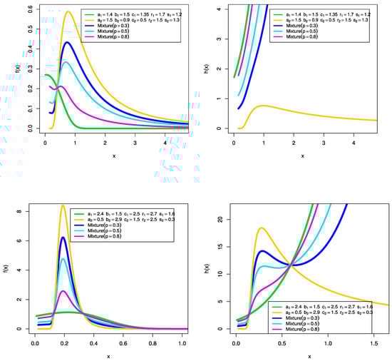
Figure 1.
Some representative PDF and hrf plots MEKGEKF distribution.
From these plots, one can observe that the PDF of MEKGEKF distribution is unimodal and right skewed. Additionally, from the hrf plots it is observed that the hrf and the MEKGEKF distribution are decreasing, increasing, unimodal, and inverse bathtub shaped.
Laplace Transformation for MEKGEKF Model
Laplace transformation is a useful tool in probability and statistics. In this section, we begin our discussion by driving the Laplace transform for the proposed MEKGEKF model. From (6) of the MEKGEKF density, the associated Laplace transform will be
where
where
where, again,
where
Combining () and (), we get:
Next, consider the following:
Combing (10), (11), and (12) in (6), we get:
on using Mathematica.
Therefore,
Observe that (13) is not available in closed form.
Therefore, the Laplace transformation for the MEKGEKF model is given by where and are given by (13) and (14), respectively.
3. Maximum Likelihood Estimation of MEKGEKF Distribution under Progressive Type II Censoring
Assume that n units are subjected to a life test at time 0, and that the experimenter determines the quantity , the number of failures to be observed, ahead of time. Next, units are now randomly deleted from the remaining n-1 surviving units at the time of first failure; units from the remaining units are randomly deleted at the second failure. The test will continue until the mth failure has occurred. The remaining units are deleted at this time. and m are prefixed in this censoring scheme. The m failure times obtained from a progressive type II censoring scheme was arranged. Progressive type II censored ordered statistics are the names given to the values acquired as a result of this type of censoring scheme. This scheme reduces to a classical type II right censoring technique if so that . Additionally, if , the progressively type II censoring method simplifies to the case of a complete sample (m = n, i.e., the case of no censoring).
Let be a progressively type II censored sample, with the progressive censoring scheme Based on progressively type II censored samples obtained from the MEKGEKF distributions, from (6), the associated likelihood function will be:
where . Here, we get the log likelihood function without the constant term. To make things easier, we’ll use the natural logarithm of the likelihood function, , which is as follows:
The maximum-likelihood estimates (MLEs) of the parameter vector are calculated by taking partial derivatives of (16) w.r.t. the parameters, and setting them equal to zero. These equations cannot be solved analytically, and we need to consider adopting any iterative techniques, such as simulated annealing, or Newton–Raphson type algorithm. In this case, we adopt the second choice for the iterative algorithm, i.e., the Newton–Raphson method.
Fisher Information Matrix (FIM)
The FIM is important in the calculation of uncertainty and other aspects of estimation for a wide range of statistical methods and applications, including parameter estimation, and experimental design for more details see [19].
The FIM is an excellent indicator of how much information sample data can provide regarding parameters. Assume is the density function and is associated with the log-likelihood function. We can define the expected FIM, I, as follows:
We may investigate the global maxima of the log-likelihood by setting different starting values for the parameters. The FIM will be required for interval estimation. The elements of observed FIM (since expected values are different to calculate), can be obtained from the authors upon request. The asymptotic distribution of is , under the standard regularity conditions, where is the expected information matrix, and is the observed information matrix. The multivariate normal distribution can be used to construct approximate confidence intervals for the individual parameters. The asymptotic variance-covariance matrix of the MLE can be obtained from the inverse of the observed FIM as: .
Then, based on the asymptotic normality of the MLE, a approximate confidence interval for the parameters (say) can be obtained as:
4. Bayesian Estimation
In recent years, Bayes’ paradigm has gained popularity in a range of fields, including engineering, clinical medicine, biology, and so on. Its ability to analyze earlier (prior) data makes it particularly useful in dependability studies, where data availability is one of the most significant challenges. This section develops the Bayes estimates and corresponding credible intervals of the model parameters,
4.1. Prior Information and Loss Function
As the gamma distribution can take on a variety of shapes depending on its parameter values, employing independent gamma priors is straightforward and can result in more expressive posterior density estimates. As a result, we consider gamma density priors, which are more flexible and convenient than other less informative independent prior distributions, in order to tailor support for the MEKGEKF distribution parameters. Therefore, the independent gamma priors for the MEKGEKF distribution parameters, are assumed to be , respectively. A logical assumption for an appropriate prior for the mixing weight parameter p could be a uniform (0,1), which we have assumed in the context. The joint prior in this case will be:
where , that reflect the prior knowledge of the unknown parameters . It is assumed that are known and non-negative. Regarding the use of such priors in this context, see [20,21] and the references cited therein.
Next, we consider an appropriate loss function. According to [22], the choice of the symmetric loss function (SLF) is a critical issue in Bayesian analysis. The squared error loss function (SEL) is the most commonly utilized SLF that is considered in this study for estimating the unknown parameters which is given by:
where is a close approximation of . The objective is to use the above function to calculate the Bayesian estimates of the parameters to be obtained as posterior mean of On the other hand, any other loss functions, such as LINEX, composite, precautionary loss functions can be readily added as appropriate.
4.2. Posterior Analysis by SLF
Observing the progressively type II censored sample data from the likelihood function in (15), and combining with the prior knowledge as given earlier, yields the following form of the joint posterior density function. are the MEKGEKF density and the CDF given in (4) and (5), respectively.
The Bayes estimator of (i.e., the parameter vector) will be the posterior expectation of , denoted by under the SEL function. In order to obtain these estimators, the marginal posterior distributions for each of the parameters in must be collected. However, explicit expressions for the marginal PDFs for each of the unknown parameters cannot be obtained simultaneously due to interactable and complicated mathematical computation. As a result, we compute Bayesian estimates and credible intervals using simulation methods such as MCMC techniques.
One of the most useful MCMC algorithms is the Metropolis–Hastings (MH) algorithm which is used to generate random samples using the posterior density distribution. Additionally, an independent proposal distribution to approximate Bayesian estimates is applied to create the associated Highest Posterior Density (HPD) credible intervals. Furthermore, this method provides a chain form of the Bayesian estimates that are easy to utilize in practice. For more information on this algorithm, see [23,24] and the references cited therein.
5. Monte Carlo Simulation
To compare the performance of the different estimators mentioned earlier, under both the classical and Bayesian paradigm, we build a Monte Carlo simulation of maximum likelihood estimates for MEKGEKF distribution based on a progressively type II samples obtained under different schemes at first.
5.1. Simulation Study
Several simulation studies were carried out to evaluate the performance of the MLE based on various censoring schemes. We offer a detailed simulation study that compares the performance of the likelihood estimation approach with Bayesian inference assuming gamma prior distributions for each parameter. In simulation studies, the sample size (n), censored progression size (m), replication (N), and different techniques are all changed in a systematic way.
5.2. Simulation Design
A censored sample for the MEKGEKF model in the simulation inquiry was created using a progressively type II censored sample. We define the scheme with replication, N = 10,000, as follows:
- -
- The total sample size (n) was altered, resulting in two levels of n = 100 and 200.
- -
- In the presence of and , the size of the progressive censored sample (m) was changed, generating two levels: m = 70, and 85, when n = 100, and m = 150 and 185, when n = 200.
- -
- The following two censored sample techniques were considered:
- -
- Scheme I: , .
- -
- Scheme II: , .
- -
- We create two models, one with parameters and the other with parameters The true values of the parameters for the first model are and and 0.7.
- -
- We determine the length of the confidence interval using a 95% confidence level.
5.3. Simulation Study
For the Monte Carlo simulation, the estimation methods indicated in Section 3 and Section 4 were employed to estimate the model parameters. To acquire the desired MLEs, the iterative NR approach is numerically implemented (as closed form expressions for the MLE are not available in this case) using the ‘maxLik’ package in R. The regularity conditions are satisfied for approximate normality assumption, asymptotic confidence intervals for each of the parameters are computed using the formula as given in Section 3. MCMC techniques and the MH algorithm were used to create Bayesian estimators based on the independent gamma priors as distributed earlier.
5.4. Comment on the Simulation Study
For each predicted model parameter, the bias, the mean square error (MSE), and the length of confidence intervals (L.CI) were calculated. Table 1 and Table 2 show the estimated values for the eight parameters of MEKGEKF model. The predicted results for the 11 parameters are shown in Table 3 and Table 4. There is some interesting information that can be observed from these tables. As the sample size n and m increases, the estimates become more accurate, implying that they are asymptotically unbiased which a desirable property. When we increase the value of parameter , the mixing component to 1, the bias, MSE and L.CI decrease. Furthermore, the MSE decreases as the sample size increases in all situations, implying that these estimates are consistent. When comparing between the two estimates, we observe that the Bayes estimates have the lowest MSE in the vast majority of cases. The L.CI for estimates approaches 0 as it grows, indicating that the CI is the shortest. However, we cannot say that the Bayesian method will be uniformly better in all situations.

Table 1.
MLE and the Bayesian estimates for eight parameters of MEKGEKF model based on a progressively Type II censoring scheme: scheme II.
Table 2.
MLE and the Bayesian estimates for eight parameters of MEKGEKF model based on a progressively type II censoring scheme: scheme I.
Table 3.
MLE and the Bayesian estimates for 11 parameters of MEKGEKF model based on a progressively type II censoring scheme: scheme II.
Table 4.
MLE and the Bayesian estimates for 11 parameters of MEKGEKF model based on a progressively type II censoring. scheme: scheme I.
6. Real Data Applications
We consider several lifetime data sets in this section to demonstrate how well this new finite mixture distribution fits for illustrative purposes. For the components (of the mixture) of the distribution’s efficacy, we calculated the Akaikes information criterion (AIC), the Bayesian information criterion (BIC), the Hannan Quinn information criterion (HQIC), and the Kolmogorov–Smirnov (K-S) values. The parameters were estimated using the MLE method, and the MLE optimizations are done using the Nelder–Mead technique, which is a numerical approach for finding the global maximum of an objective function in a multidimensional space, and the R software is utilized.
6.1. Operation Data on Jobs Made of Iron Sheet
The data set consists of 50 observations (in millimeters), the hole diameter is 12 mm, and the sheet thickness is 3.15 mm, as reported in [25]. The data values are: 0.04, 0.02, 0.06, 0.12, 0.14, 0.08, 0.22, 0.12, 0.08, 0.26, 0.24, 0.04, 0.14, 0.16, 0.08, 0.26, 0.32, 0.28, 0.14, 0.16, 0.24, 0.22, 0.12, 0.18, 0.24, 0.32, 0.16, 0.14, 0.08, 0.16, 0.24, 0.16, 0.32, 0.18, 0.24, 0.22, 0.16, 0.12, 0.24, 0.06, 0.02, 0.18, 0.22, 0.14, 0.06, 0.04, 0.14, 0.26, 0.18, 0.16.
We conjecture that the data have interesting characteristics if we divide it into two parts and also conjecture that a mixing distribution (finite mixture) will be adequate to explain the hidden characteristics for the data. The two-component mixture of EKF and EKG distribution was applied to the data set given as.
Subpopulation I: 0.04, 0.06, 0.12, 0.22, 0.08, 0.26, 0.14, 0.08, 0.32, 0.14, 0.16, 0.12, 0.24, 0.16, 0.08, 0.16, 0.32, 0.24, 0.22, 0.24, 0.02, 0.22, 0.06, 0.14, 0.26; these data are applied to EKF distribution.
Subpopulation II: 0.02, 0.14, 0.08, 0.12, 0.24, 0.04, 0.16, 0.26, 0.28, 0.24, 0.22, 0.18, 0.32, 0.14, 0.24, 0.16, 0.18, 0.16, 0.12, 0.06, 0.18, 0.14, 0.04, 0.18, 0.16; these data are applied to EKG distribution.
From Table 5 and Table 6, we note that EKF is the best model for each data, but the p-value for EKG is larger than EKF for data set II. Therefore, the first distribution EKF is good for data set I, and the second distribution EKG is good for data set II in the mixture model. However, either of the distributions cannot provide a good fit for the entire data set.
Table 5.
MLE, stander error (SE), KS test, and p-value for different sets for the hole data.
Table 6.
Goodness-of-fit measures, AIC, BIC, CAIC, and HQIC for the hole diameter data.
Table 6 shows the different goodness-of-fit measures values as AIC, BIC, CAIC, and HQIC for EKG and EKF distribution for the hole diameter data. Here, we conclude that the EKF model is better than the EKG model.
Figure 2 and Figure 3 show the Estimated CDF and PDF for EKG and EKF distribution for Subpopulation I and estimated CDF and PDF for EKG and EKF distribution for Subpopulation II. While, the PP-plot for EKG and EKF distribution for Subpopulation I and the PP-plot for EKG and EGF distribution for Subpopulation II are indicated in Figure 4 and Figure 5, respectively.
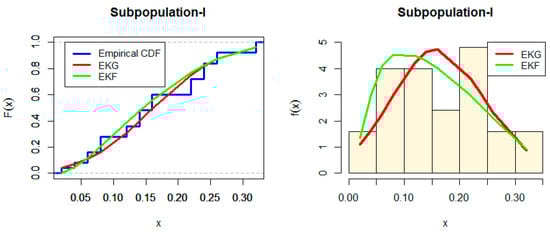
Figure 2.
Estimated CDF and PDF for EKG and EKF distribution for Subpopulation I.
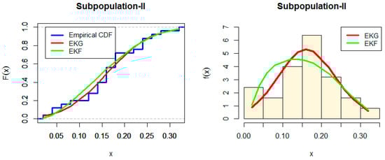
Figure 3.
Estimated CDF and PDF for EKG and EKF distribution for Subpopulation II.
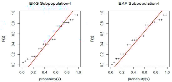
Figure 4.
PP-plot for EKG and EKF distribution for Subpopulation I.
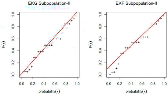
Figure 5.
PP-plot for EKG and EGF distribution for Subpopulation II.
Table 7 report the MLE and Bayesian estimation parameters of mixture of exponentiated Kumaraswamy Gompertz and exponentiated Kumaraswamy Fréchet distribution. From the reported results, we conclude that the Bayesian estimation is preforming better than the MLE where the standard error (SE) values are smaller compared the SE values obtained under the MLE method.
Table 7.
MLE and the Bayesian estimates for the fitted MEKGEKF model.
From the above summary measures, it appears that the MEKGEKF model might be a reasonably good fit for the data.
6.2. Wire Data
In the Wire Fatigue Experiment [26], a 48-stranded stainless-steel wire was ruptured by clamping it in needle-nose pliers and hanging a 1.65-pound weight on it while using 3/4 of a liter of water, then a 2.2-pound weight while using 1 liter of water. The pliers were spun clockwise and counterclockwise by 180 degrees. The number of half twists that resulted in total rupture (failure) was counted. For the Wire Fatigue Experiment, the wire data represent the number of half twists to total rupture as follows: 37, 30, 27, 51, 10, 24, 15, 14, 34, 34, 42, 25, 15, 13, 16, 12, 27, 21, 37, 35, 18, 17, 17, 13, 35, 27, 41, 41, 14, 17, 20, 16, 28, 24, 32, 24, 17, 19, 15, 20, 45, 39, 27, 33, 18, 13, 11, 13.
From Table 8, we note that EKF is the fitting model for Wire data, but the p-value of EKF is larger than EKG for Wire data. Figure 6 and Figure 7 shows that the shape of the probability density function is bimodal for both EKG and EKF distribution but the original data shape is uni-modal. Table 9 shows different goodness-of-fit measures values such as the AIC, BIC, CAIC, and the HQIC for EKG and EKF distribution for the hole diameter data.
Table 8.
MLE with standard error (SE) and KS test for different sets and different model for Wire data.
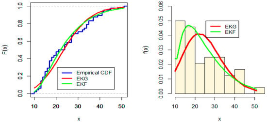
Figure 6.
Estimated CDF and PDF for EKG and EKF distribution for Wire data.
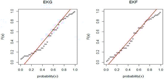
Figure 7.
PP-plot for EKG and EGF distribution for Wire data.
Table 9.
AIC, BIC, CAIC, and HQIC for different sets and different model for Wire data.
Table 10 illustrate the MLE and the Bayesian estimates for the fitted MEKGEF model for the Wire data. Consequently, we conclude that the EKF is petter than EKG model. However, from the above summary, it can be said that component-wise, either of the EKG and the EKF might not adequately fit the data. Consequently, we conjecture that the 11-parameter MEKGEKF distribution in (6) will be a good fit and in the next, we fit this distribution to this data set.
Table 10.
MLE and the Bayesian estimates for the fitted MEKGEF model for the Wire data.
6.3. Australian Athletes Data Set
These data were gathered as part of a study that looked at how data on various blood parameters differed according to the athlete’s sport body size and gender. There are 202 observations on 13 variables in this data set (for more details see [27]). The variables rcc (red blood cell count), wcc (white blood cell count), and bmi (body mass index) were investigated (body mass index).
The data values are 3.80 3.90 3.90 3.91 3.95 3.95 3.96 3.96 4.00 4.02 4.03 4.06 4.07 4.08 4.09 4.09 4.10 4.11 4.11 4.12 4.13 4.13 4.14 4.15 4.16 4.16 4.17 4.17 4.19 4.20 4.20 4.21 4.23 4.23 4.24 4.24 4.25 4.26 4.26 4.27 4.27 4.30 4.31 4.31 4.32 4.32 4.32 4.35 4.36 4.36 4.37 4.38 4.38 4.39 4.40 4.40 4.40 4.41 4.41 4.41 4.42 4.42 4.44 4.44 4.44 4.45 4.45 4.46 4.46 4.46 4.46 4.46 4.48 4.49 4.50 4.50 4.51 4.51 4.51 4.51 4.52 4.53 4.54 4.55 4.56 4.57 4.58 4.62 4.63 4.63 4.63 4.64 4.66 4.68 4.71 4.71 4.71 4.71 4.73 4.75 4.75 4.76 4.77 4.77 4.78 4.81 4.81 4.82 4.82 4.83 4.83 4.83 4.83 4.84 4.86 4.86 4.87 4.87 4.87 4.87 4.87 4.87 4.88 4.89 4.89 4.90 4.90 4.91 4.91 4.92 4.93 4.93 4.94 4.95 4.95 4.96 4.97 4.97 4.98 4.99 5.00 5.00 5.00 5.01 5.01 5.01 5.02 5.02 5.03 5.03 5.03 5.03 5.04 5.04 5.08 5.09 5.09 5.09 5.10 5.11 5.11 5.11 5.11 5.11 5.13 5.13 5.13 5.13 5.16 5.16 5.16 5.16 5.17 5.17 5.18 5.21 5.21 5.22 5.22 5.24 5.24 5.25 5.29 5.31 5.32 5.33 5.33 5.34 5.34 5.34 5.34 5.38 5.40 5.48 5.48 5.49 5.50 5.59 5.66 5.69 5.93 6.72.
From Figure 8 and Figure 9, it appears that, component-wise, EKG and EKF will not provide an adequate fit to the given data. The p-value in Table 11 also supports this assessment. As before, we conjecture that the 11 parameter MEKGEKF distribution might provide a good fit to the data. We fit the proposed distribution and the goodness-of-fit measures are reported in Table 12. The MLE and the Bayesian estimates for the fitted MEKGEF model for the Australian athletes data are shown in Table 13.
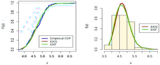
Figure 8.
Estimated CDF and PDF for EKG and EKF distribution for Australian Athletes data.
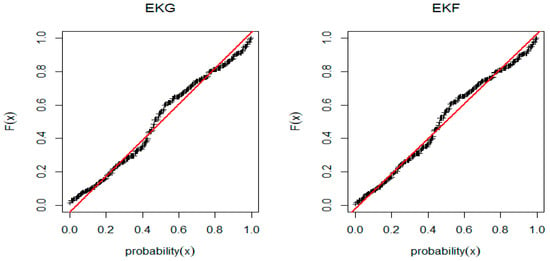
Figure 9.
PP-plot for EKG and EGF distribution for Australian Athletes data.
Table 11.
MLE with standard error (SE) and KS test for different sets and different model for Australian athletes data set.
Table 12.
AIC, BIC, CAIC, and HQIC for different sets and different model for Australian athletes data set.
Table 13.
MLE and the Bayesian estimates for the fitted MEKGEF model for the Australian athletes data.
From the above summary measures, it appears that the proposed distribution given in (6) is a reasonable model to fit the above data.
7. Concluding Remarks
Classical and Bayesian inferences for finite mixture models in the case of absolutely continuous probability models as subpopulations is not new in the literature except for the fact that probability distribution(s) defined on the unit interval (0,1) has not been considered effectively earlier. In this paper, we discuss the utility of a finite mixture model for which the components are also some mixtures with Kumaraswamy distribution as one of the mixing components under the frequentist approach, the method of the maximum likelihood is adopted while for the Bayesian estimation, independent gamma priors are considered for all the model parameters of the derived model which we call the MEKGEKF distribution. The performance of both these estimation methods are assessed in the light of a progressively censored Type II random samples drawn from the newly developed probability model. From the simulation study (under various parameter settings and various censoring scheme), it appears that this MEKGEKF distribution might be useful in analyzing certain dataset(s) for which either or both of its component distributions will be inadequate to completely explain the data.
Author Contributions
All authors have contributed equally. All authors have read and agreed to the published version of the manuscript.
Funding
This research was funded by Princess Nourah bint Abdulrahman University Researchers Supporting Project number (PNURSP2022R50), Princess Nourah bint Abdulrahman University, Riyadh, Saudi Arabia.
Institutional Review Board Statement
Not applicable.
Informed Consent Statement
Not applicable.
Data Availability Statement
The data used to support the findings of this study are included within the article.
Acknowledgments
Princess Nourah bint Abdulrahman University Researchers Supporting Project number (PNURSP2022R50), Princess Nourah bint Abdulrahman University, Riyadh, Saudi Arabia).
Conflicts of Interest
The authors declare no conflict of interest.
References
- Pearson, K. Contributions to the Mathematical theory of Evolution. Philos. Trans. R. Soc. Lond. A 1984, 185, 71–110. [Google Scholar]
- Kao, J. A Graphical Estimation of Mixed Weibull Parameters in Life-Testing of Electron Tubes. Technometrics 1959, 1, 389–407. [Google Scholar] [CrossRef]
- Ahmed, K.E.; Jaheen, Z.F.; Mohammed, H.S. Bayesian estimation under a mixture of Bur type XII distribution and its reciprocal. J. Stat. Comput. Simul. 2012, 81, 2121–2130. [Google Scholar] [CrossRef]
- Ristic, M.M.; Balakrishnan, N. The gamma- exponentiated exponential distribution. J. Stat. Comput. Simul. 2012, 82, 1191–1206. [Google Scholar] [CrossRef]
- Kundu, D. Bayesian inference and life testing plan for Weibull distribution in presence of progressive censoring. Technometrics 2008, 50, 144–154. [Google Scholar] [CrossRef]
- Raqab, M.Z.; Asgharzadeh, A.R.; Valiollahi, R. Prediction for Pareto distribution based on progressively Type-II Censored Samples. Comput. Stat. Data Anal. 2010, 54, 1732–1743. [Google Scholar] [CrossRef]
- Balakrishnan, N.; Aggarwala, R. Progressive Censoring, Theory, Methods and Applications; Birkhauser: Boston, MA, USA, 2007. [Google Scholar]
- Balakrishnan, N. Progressive Censoring Methodology: An Appraisal. TEST 2007, 16, 211–296. [Google Scholar] [CrossRef]
- Johnson, L.G. Theory and Technique of Variation Research; Elsevier: Amsterdam, The Netherlands, 1964. [Google Scholar]
- Pradhan, B.; Kundu, D. On progressively censored generalized exponential distribution. TEST 2009, 18, 497–515. [Google Scholar] [CrossRef]
- Pradhan, B.; Kundu, D. Inference and optimal censoring schemes for progressively censored Birnbaum–Saunders distribution. J. Stat. Plan. Inference 2013, 143, 1098–1108. [Google Scholar] [CrossRef]
- Cordeiro, G.M.; de Castro, M. A New Family of Generalized Distributions. J. Stat. Comput. Simul. 2011, 81, 883–898. [Google Scholar] [CrossRef]
- Cordeiro, G.M.; Nadarajah, S.; Ortega, E.M. The Kumaraswamy Gumbel distribution. Stat. Methods Appl. 2012, 21, 139–168. [Google Scholar] [CrossRef]
- Tahir, M.; Almanjahie, I.M.; Abid, M.; Ahmad, I. On Estimation of Three-Component Mixture of Distributions via Bayesian and Classical Approaches. Math. Probl. Eng. 2021, 9944008. [Google Scholar] [CrossRef]
- Tahir, M.H.; Nadarajah, S. Parameter induction in continuous univariate distributions: Well-established G families. Ann. Braz. Acad. Sci. 2015, 87, 539–568. [Google Scholar] [CrossRef] [PubMed]
- Hussein, M.; Elsayed, H.; Cordeiro, G. A new family of continuous distribution: Properties and estimation. Symmetry 2022, 14, 276. [Google Scholar] [CrossRef]
- Alzaatreh, A.; Lee, C.; Famoye, F. A new method for generating families of continuous distribution. Metron 2013, 71, 63–79. [Google Scholar] [CrossRef] [Green Version]
- Nadarajah, S.; Rocha, R. Newdistns: An R Package for New Families of Distributions. J. Stat. Softw. 2016, 69, 1–32. [Google Scholar] [CrossRef] [Green Version]
- Spall, J.C. Feedback and Weighting Mechanisms for Improving Jacobian Estimates in the Adaptive Simultaneous Perturbation Algorithm. IEEE Trans. Autom. Control 2009, 54, 1216–1229. [Google Scholar] [CrossRef]
- Almetwally, E.M.; Abdo, D.A.; Hafez, E.H.; Jawa, T.M.; Sayed-Ahmed, N.; Almongy, H.M. The new discrete distribution with application to COVID-19 Data. Results Phys. 2022, 32, 104987. [Google Scholar] [CrossRef]
- Metwally AS, M.; Hassan, A.S.; Almetwally, E.M.; Kibria, B.M.; Almongy, H.M. Reliability Analysis of the New Exponential Inverted Topp–Leone Distribution with Applications. Entropy 2021, 23, 1662. [Google Scholar] [CrossRef]
- Moore, D.; Papadopoulos, A.S. The Burr Type XII distribution as a failure model under various loss functions. Microelectron. Reliab. 2000, 40, 17–22. [Google Scholar] [CrossRef]
- Gelman, A.; Carlin, J.B.; Stern, H.S.; Rubin, D.B. Bayesian Data Analysis, 2nd ed.; Chapman and Hall/CRC: Boca Raton, FL, USA, 2004. [Google Scholar]
- Lynch, S.M. Introduction to Applied Bayesian Statistics and Estimation for Social Scientists; Springer: New York, NY, USA, 2007. [Google Scholar]
- Dasgupta, R. On the distribution of burr with applications. Sankhya B 2011, 73, 1–19. [Google Scholar] [CrossRef]
- Abernethy, R.B. The New Weibull Handbook: Reliability & Statistical Analysis for Predicting Life, Safety, Survivability, Risk, Cost, and Warranty Claims, 5th ed.; Abernethy: North Palm Beach, FL, USA, 2010. [Google Scholar]
- Telford, R.D.; Cunningham, R.B. Sex, sport and body-size dependency of hematology in highly trained athletes. Med. Sci. Sports Exerc. 1991, 23, 788–794. [Google Scholar] [CrossRef] [PubMed]
Publisher’s Note: MDPI stays neutral with regard to jurisdictional claims in published maps and institutional affiliations. |
© 2022 by the authors. Licensee MDPI, Basel, Switzerland. This article is an open access article distributed under the terms and conditions of the Creative Commons Attribution (CC BY) license (https://creativecommons.org/licenses/by/4.0/).