Analytic Approximation for American Straddle Options

Abstract

This paper looks at adapting a recent approach found in the literature for pricing short-term American options to price American straddle options with two free boundaries. We provide a series solution in which explicit formulas for the coefficients are given. Hence, no complicated, recursive systems or nonlinear integral equations need to be solved, and the method efficiently provides fast solutions. We also compare the method with a numerical method and find that it gives very accurate prices not only for the option value, but also for the critical stock prices.

1. Introduction

A European straddle is a strategy that involves buying both a European call option and a European put option both with the same strike price and expiration date. The strategy is extremely popular in a volatile market as the more the underlying asset moves from the chosen strike price, the higher the value of the straddle. The European straddle can be exercised only at the expiry time, at which time the payoff is $max(S-X,X-S)$, where S is the value of the underlying asset at expiry and X is the strike price. The value of a European straddle is simply the sum of the component call and put options, which can be calculated using the famous Black–Scholes formulas (see, e.g., Kwok [1]). An American straddle also has the payoff at expiry of $max(S-X,X-S)$, but it can be exercised at any time before expiry and so there exist free boundaries, or optimal exercise boundaries (OEBs), which mark the borders between holding and exercising the straddle. Hence, its value is not simply the combination of an American call option and an American put option.

American options offer investors a means to offset their financial risk as well as a means to attain higher returns should their opinion on the market direction be correct. Given their immense popularity worldwide, it is as expected that their pricing has attracted considerable research. Unfortunately to date, even for the vanilla American call and put options, no fully analytical solution for their price and optimal exercise boundaries have been found. While the American call and put options each have one free boundary, the American straddle has two: an upper one, similar to that for a call option and a lower one, similar to that for a put option. This means the valuation of American straddles is even more challenging.

In 2002, Alobaidi and Mallier [2] attempted to use partial Laplace transforms on the Black–Scholes partial differential Equation (PDE) to find the value of the straddle option price. However they were not able to invert the value function in Laplace format. Then in 2006, the same authors [3] used a method due to Kim [4] to formulate an integral representation for the price of straddle options near expiry. They obtained a set of four coupled nonlinear (Volterra of the second kind) integral equations governing the locations of the free boundaries, which were then solved asymptotically to find their locations close to expiry. Both the value function and the free boundaries were written as series in functions of time-to-expiry, and to determine each coefficient involved solving complicated nonlinear systems of equations.

A related derivative to the American straddle is the American strangle. The payoff of strangle options is defined as $max({(S-K)}^{+},{(L-S)}^{+})$, where K is the higher strike price and L is the lower strike price, satisfying $K>L$. Hence, the strangle is similar to the straddle, but uses different strike prices. From the definition of the payoff function, this option will be in-the-money when the stock price S is in the regions $S<L$ and $S>K$.

The strangle was studied by Chiarella and Ziogas [5] who used the Fourier transform method to formulate a coupled integral equation system for the value of the strangle’s two free boundaries. The system was solved numerically and the free boundaries were then used to find the price of the American strangle.

Additionally, Detemple [6] got the same early exercise premium representation for the value of American strangle options as was found in Chiarella and Ziogas [5], which again was suitable for applying a numerical method to calculate the option price.

Numerical methods, such as lattice methods, have also been studied for pricing American strangles. This includes the work of Gao et al. [7], who used lattice methods for pricing American strangles and then compared the results with the least square Monte Carlo method via numerical examples.

More recently, Kang et al. [8] attempted to price American strangles using Laplace–Carson transforms. However, although they derived in the Laplace–Carson space an analytic expression of the value function and a nonlinear system of equations in the transformed variables of the two free boundaries, this nonlinear system had to be solved using numerical Laplace inversion techniques.

The majority of the above references used the integral equation approach to price the American strangle or straddle. However, this generally means no closed-form solutions for the optimal exercise boundaries and value function. The nonlinear integral equations are also difficult to solve efficiently using numerical methods. In a different approach, Ma et al. [9] constructed upper and lower bounds for the value of an American strangle and proposed an algorithm to approximate the early exercise boundary of the American strangle option.

Also using an integral equation approach, Qiu [10] showed that the double optimal stopping boundaries for American strangle and straddle options with finite maturity can be described as the unique pair of solution to a system of two nonlinear integral equations. These equations were derived using an early exercise premium representation. To calculate the double free-boundaries in the system of two integral equations he introduced a numerical method. Through computer simulation he showed intuitively that with respect to time, the lower and upper boundaries were increasing and decreasing, respectively. He also showed (in his Theorem 8) that for American strangle options, when time t approaches maturity T, the upper and lower free-boundaries converge respectively to the early exercise boundaries of the American call and put options, i.e., $max(K,rK/q),min(L,rL/q),$ where $r,q$ are the risk-free interest rate and continuous dividend yield, respectively.

In this paper, we adapt and improve on the method of Medvedev and Scaillet [11], who proposed a new analytical approximation method to price short-term American put options. The main idea behind their proposal was to replace the optimal exercise rule with a simple suboptimal exercise rule so that as soon as the option’s moneyness reached some desired level, then the option should be exercised. The American option price was given as an asymptotic series with respect to time to maturity. They say their method [11] ‘is both computationally tractable and general enough to be successfully applied to a three factor diffusion model without jumps’. However a major weakness of the method is that complicated recursive systems need to be solved in order to calculate the coefficients of their asymptotic series. With investors requiring quick answers, this is a significant issue. In this paper, we modify their method to present an analytic approximation to American straddle options. However, rather than solving a recursive system, we provide explicit formulas for the coefficients in the series solution. Free boundary problems are notoriously hard to solve and the American straddle option problem has two free boundaries: an upper and a lower. The solution for the options as well as the critical stock prices are derived and then compared to those found by the numerical Crank–Nicolson method. Our solutions are found to be very accurate and the solution method highly efficient compared to the time-consuming numerical method. We also examine the asymptotic behavior of the free boundaries as time to expiry tends to zero.

2. The Mathematical Model and Solution

We now present the main result of the paper, in which we present the series representation for the American straddle option price. Explicit formulas are given for the coefficients in the series.

We let $V(S,t)$ be the price of an American straddle option with exercise price X and expiry T and assume that the stock price S follows the risk-neutral lognormal process, i.e.,

$$dS/S=(r-q)dt+\sigma dZ.$$

(1)

In (1), $r,q$ and $\sigma$ are, respectively, the constant risk-free interest rate, dividend yield and volatility and $dZ$ is an increment in a Wiener process Z, under a risk-neutral measure. Then, if we denote the upper optimal exercise boundary (OEB) by $S_u\left(t\right)$ and the lower optimal exercise boundary by $S_l\left(t\right)$ then in the continuation region, $S_l\left(t\right)\le S<S_u\left(t\right)$ the value $V(S,t)$ satisfies the Black–Scholes Equation (see Appendix A)

$$V_t+\frac{{\sigma }^2{S}^2}{2}{V}_{SS}+(r-q)S{V}_S-rV=0,$$

(2)

subject to

$$\begin{array}{ccc}\hfill V(S,T)& \hfill =\hfill & max(X-S,S-X),\hfill \end{array}$$

(3a)

$$\begin{array}{ccc}\hfill V(S_u\left(t\right),t)& \hfill =\hfill & S_u\left(t\right)-X,\hfill \end{array}$$

(3b)

$$\begin{array}{ccc}\hfill V_S(S_u\left(t\right),t)& \hfill =\hfill & 1,\hfill \end{array}$$

(3c)

$$\begin{array}{ccc}\hfill V(S_l\left(t\right),t)& \hfill =\hfill & X-S_l\left(t\right),\hfill \end{array}$$

(3d)

$$\begin{array}{ccc}\hfill V_S(S_l\left(t\right),t)& \hfill =\hfill & -1.\hfill \end{array}$$

(3e)

In pricing an American put option with price $P(S,t)$ and free boundary $S_f\left(t\right)$, Medvedev and Scaillet [11] replaced the smooth-pasting condition $P_S(S_f\left(t\right),t)=-1$ by an explicit exercise rule and assumed that the OEB had the form

$$S_f\left(t\right)=X{e}^{-y\sigma \sqrt{T-t}},$$

(4)

where y is a decision variable determining the suboptimal rule. Hence, the American put option was treated as a barrier put option that is exercised when the normalized level of moneyness, $\frac{ln\left(\frac{X}{S}\right)}{\sigma \sqrt{T-t}}$, reaches the barrier level y. The same application is used in our paper where there is now an upper and lower barrier. We will use a similar idea for both of the free boundaries of the straddle option and, unlike Medvedev and Scaillet, give explicit formulas for the coefficients in the series representation for the American straddle. The following theorem gives our main result.

Theorem 1.

Let $x=ln(X/S)$ and $\tau =T-t.$ The approximation to the short-term American straddle option price in $S_l\left(t\right)\le S\le S_u\left(t\right),$ where $S_u\left(t\right)$ and $S_l\left(t\right)$, respectively, are the upper and lower OEBs is

$$V(x,\tau )=\underset{y⩾\frac{-x}{\sigma \sqrt{\tau }},z⩾\frac{x}{\sigma \sqrt{\tau }}}{max}V(x,\tau ;y,z)=V(x,\tau ;\widehat{y},\widehat{z}),$$

(5)

where

$$\begin{array}{ccc}\hfill V(x,\tau ;y,z)& =& e^{-q\tau }{e}^{Ax+B\tau }{e}^{\frac{-x^2}{2{\sigma }^2\tau }}\sum _{i=1}^{\infty }{\tau }^{i/2}\left[C_{i}M\left(\frac{1+i}{2},\frac{1}{2},\frac{x^2}{2{\sigma }^2\tau }\right)+D_{i}U\left(\frac{1+i}{2},\frac{1}{2},\frac{x^2}{2{\sigma }^2\tau }\right)\right]\hfill \\ & & forln\left(\frac{X}{S_u}\right)\le x\le 0(i.e.,X\le S\le S_u),\hfill \\ & =& e^{-q\tau }{e}^{Ax+B\tau }{e}^{\frac{-x^2}{2{\sigma }^2\tau }}\sum _{i=1}^{\infty }{\tau }^{i/2}\left[\left(C_i+\frac{2D_i\sqrt{\pi }}{\mathsf{\Gamma }(1+i/2)}\right)M\left(\frac{1+i}{2},\frac{1}{2},\frac{x^2}{2{\sigma }^2\tau }\right)\right.\hfill \\ & & -D_i\left.U\left(\frac{1+i}{2},\frac{1}{2},\frac{x^2}{2{\sigma }^2\tau }\right)\right]\hfill \\ & & for 0<x\le ln\left(\frac{X}{S_l}\right)(i.e.,S_l\le S<X),\hfill \end{array}$$

(6)

with $A=\frac{r-q-\frac{{\sigma }^2}{2}}{{\sigma }^2},B=-\frac{{(r-q+\frac{{\sigma }^2}{2})}^2}{2{\sigma }^2}$ and M and U represent the confluent hypergeometric functions, Kummer-M and Kummer-U, respectively (see [12]).

The coefficients $C_i$ and $D_i$ are given by

$$\begin{array}{ccc}\hfill C_i& =& \frac{-\left[2e^{z^2/2}X\left(\sqrt{\pi }p({\widehat{ϵ}}_i-{\gamma }_i)M^z-\frac{\mathsf{\Gamma }(1+i/2)}{2}\{({\varphi }_i-{\psi }_i)U^y+p{U}^z({\widehat{ϵ}}_i-{\gamma }_i)\}\right)\right]}{\left([2\sqrt{\pi }{M}^y-\mathsf{\Gamma }(1+i/2)U^y]M^z-\mathsf{\Gamma }(1+i/2)U^z{M}^y\right)}\hfill \end{array}$$

(7)

$$\begin{array}{ccc}\hfill D_i& =& \frac{e^{z^2/2}X\left[({\psi }_i-{\varphi }_i)M^y+p{M}^z({\widehat{ϵ}}_i-{\gamma }_i)\right]\mathsf{\Gamma }(1+i/2)}{\left([2\sqrt{\pi }{M}^z-\mathsf{\Gamma }(1+i/2)U^z]M^y-\mathsf{\Gamma }(1+i/2)U^y{M}^z\right)}\hfill \end{array}$$

(8)

where

$$\begin{array}{ccc}\hfill p& =& exp\left(\frac{y^2-z^2}{2}\right)\hfill \end{array}$$

(9a)

$$\begin{array}{ccc}\hfill M^y& =& M\left(\frac{1+i}{2},\frac{1}{2},\frac{y^2}{2}\right),M^z=M\left(\frac{1+i}{2},\frac{1}{2},\frac{z^2}{2}\right),\hfill \end{array}$$

(9b)

$$\begin{array}{ccc}\hfill U^y& =& U\left(\frac{1+i}{2},\frac{1}{2},\frac{y^2}{2}\right),U^z=U\left(\frac{1+i}{2},\frac{1}{2},\frac{z^2}{2}\right),\hfill \end{array}$$

(9c)

$$\begin{array}{ccc}\hfill {\widehat{ϵ}}_i& =& \sum _{j=0}^i{ϵ}_j{b}_{i-j},{\gamma }_i=\sum _{j=0}^i{b}_j{\left({\beta }^{\prime }\right)}_{i-j},{\psi }_i=\sum _{j=0}^i{a}_j{b}_{i-j},\hfill \end{array}$$

(9d)

$$\begin{array}{ccc}\hfill {\varphi }_i& =& \sum _{j=0}^i{\alpha }_j{b}_{i-j},\hfill \end{array}$$

(9e)

with

$$b_n=\left\{\begin{array}{cc}0\hfill & n=1,3,5,\dots \hfill \\ \frac{{(q-B)}^{n/2}}{(n/2)!}\hfill & n=0,2,4,\dots \hfill \end{array}\right.$$

(9f)

$$a_m=\frac{{(-Az\sigma )}^m}{m!},m=0,1,2,3\dots$$

(9g)

$${ϵ}_m=\frac{{\left(Ay\sigma \right)}^m}{m!},m=0,1,2,3\dots$$

(9h)

$${\alpha }_m=\frac{{(-(1+A)z\sigma )}^m}{m!},m=0,1,2,3,\dots$$

(9i)

$${\beta }_m^{\prime }=\frac{{\left((1+A)y\sigma \right)}^m}{m!},m=0,1,2,3,\dots$$

(9j)

The upper and lower optimal exercise boundaries are given respectively by

$$S_u=X{e}^{y\sigma \sqrt{\tau }}$$

(10)

and

$$S_l=X{e}^{-z\sigma \sqrt{\tau }},$$

(11)

$y,z\ge 0$, where approximations ${\widehat{\theta }}_1,$${\widehat{\theta }}_2$ for the true early exercise level of moneyness, are given by

$${\widehat{\theta }}_1\left(\tau \right)=\arg \underset{\theta =\frac{x}{\sigma \sqrt{\tau }}}{min}[\widehat{y}(\theta ,\tau )=-\theta ],$$

(12)

and

$${\widehat{\theta }}_2\left(\tau \right)=\arg \underset{\theta =\frac{x}{\sigma \sqrt{\tau }}}{min}[\widehat{z}(\theta ,\tau )=\theta ],$$

(13)

where $\widehat{y}$ and $\widehat{z}$ are implicitly defined in (5).

Note: Outside the continuation region, the option should be exercised. Hence, for $S>S_u\left(t\right),V(S,t)=S-X$ and for $S<S_l\left(t\right),V(S,t)=X-S$.

Proof. 

It is useful to divide the continuation domain into the 2 regions $S_l\left(t\right)\le S<X$ and $X\le S\le S_u\left(t\right)$. In the continuation region of the American straddle option, the option price $V(S,t)$ satisfies Equation (2), which in

$S_l\left(t\right)\le S<X$ necessitates being solved subject to

$$V(S_l\left(t\right),t)=X-S_l\left(t\right),$$

(14)

and in $X\le S<S_u\left(t\right)$, subject to $V(S_u\left(t\right),t)=S_u\left(t\right)-X.$

Note: As indicated in (6), we will be formulating a solution of the form

$$V(\theta ,\tau )=g(\theta ,\tau )\sum _{n=1}^{\infty }{f}_n\left(\theta \right){\tau }^{n/2},$$

(15)

where $\theta =\frac{x}{\sigma \sqrt{\tau }},x=ln\left(\frac{X}{S}\right)$, and where g and $f_n$ are given functions found by comparing (15) with (6).

With $\theta$ fixed, when $\tau =0$, $g(\theta ,0)=exp(-\frac{{\theta }^2}{2})$ and $S=X$. This means the payoff $max(X-S,S-X)=0$ is implied by the form (15) and hence the final condition (3a) will be satisfied.

We also require that across the strike price we have continuity of the value of the option and its derivative, i.e.,

$$\begin{array}{ccc}\hfill \underset{S\to X^{-}}{lim}V& =& \underset{S\to X^{+}}{lim}V,\hfill \end{array}$$

$$\begin{array}{ccc}\hfill \underset{S\to X^{-}}{lim}{V}_S& =& \underset{S\to X^{+}}{lim}{V}_S.\hfill \end{array}$$

We note that continuity of the second derivative $V_{SS}$ across the strike price is also required for an exact, classical solution to the second-order PDE (2). This will be shown to follow automatically.

Making the substitutions

$$S=X{e}^{-x},t=T-\tau ,V=e^{-q(T-t)}W(x,\tau ),$$

PDE (2) becomes

$$W_{\tau }=\frac{{\sigma }^2}{2}{W}_{xx}+\left[\frac{{\sigma }^2}{2}+(q-r)\right]W_x-(r-q)W.$$

(16)

We note that a similar PDE of parabolic type was considered by Covei [13] where the author connected the considered equation with a production planning problem. We solve (16) on $(-y\sigma \sqrt{\tau },0)$ subject to $W(-y\sigma \sqrt{\tau },\tau )=X{e}^{q\tau }(e^{y\sigma \sqrt{\tau }}-1)$ and on $(0,z\sigma \sqrt{\tau })$ subject to $W(z\sigma \sqrt{\tau },\tau )=X{e}^{q\tau }(1-e^{-z\sigma \sqrt{\tau }}).$ The continuity conditions become

$$\begin{array}{ccc}\hfill \underset{x\to 0^{-}}{lim}W& =& \underset{x\to 0^{+}}{lim}W,\hfill \\ \hfill \underset{x\to 0^{-}}{lim}{W}_x& =& \underset{x\to 0^{+}}{lim}{W}_x.\hfill \end{array}$$

Now letting $W=exp(Ax+B\tau )u(x,\tau )$ where $A=\frac{r-q-\frac{{\sigma }^2}{2}}{{\sigma }^2},B=\frac{{\sigma }^2{A}^2}{2}+A(q-r+\frac{{\sigma }^2}{2})-(r-q)$ reduces (16) to the classical heat equation

$$u_{\tau }=\frac{{\sigma }^2}{2}{u}_{xx}.$$

(17)

Finally, we let $\theta =\frac{x}{\sigma \sqrt{\tau }}$ to get

$$2\tau u_{\tau }=u_{\theta \theta }+\theta u_{\theta },$$

(18)

to be solved on $-y\le \theta \le 0$ subject to

$$u(-y,\tau )=Xexp(Ay\sigma \sqrt{\tau }-B\tau )exp\left(q\tau \right)(exp\left(y\sigma \sqrt{\tau }\right)-1),$$

(19)

and on $0<\theta \le z$ subject to

$$u(z,\tau )=Xexp(-Az\sigma \sqrt{\tau }-B\tau )exp\left(q\tau \right)(1-exp(-z\sigma \sqrt{\tau })),$$

(20)

with continuity conditions

$$\begin{array}{ccc}\hfill \underset{\theta \to 0^{-}}{lim}u& =& \underset{\theta \to 0^{+}}{lim}u,\hfill \end{array}$$

$$\begin{array}{ccc}\hfill \underset{\theta \to 0^{-}}{lim}{u}_{\theta }& =& \underset{\theta \to 0^{+}}{lim}{u}_{\theta }.\hfill \end{array}$$

Equation (18) admits separable solutions of the form

$$u(\theta ,\tau )=e^{\frac{-{\theta }^2}{2}}\sum _{i=1}^{\infty }{\tau }^{\frac{i}{2}}\left[C_{i}M\left(\frac{1+i}{2},\frac{1}{2},\frac{{\theta }^2}{2}\right)+D_{i}U\left(\frac{1+i}{2},\frac{1}{2},\frac{{\theta }^2}{2}\right)\right],$$

(21)

where M and U are the confluent hypergeometric functions, Kummer-M and Kummer-U functions, respectively. In (21), we have used the separation constant ${\lambda }_i=\frac{i}{2}$ where i is a positive integer. This was chosen as power series in square root of time have been shown to be effective in solving other free boundary problems that involve linear diffusion equations (see, e.g., Tao [14]). We will use (21) to describe the solutions in $-y\le \theta \le 0$.

For $0<\theta \le z$ we use different constants and write

$$u(\theta ,\tau )=e^{\frac{-{\theta }^2}{2}}\sum _{i=1}^{\infty }{\tau }^{\frac{i}{2}}\left[F_{i}M\left(\frac{1+i}{2},\frac{1}{2},\frac{{\theta }^2}{2}\right)+G_{i}U\left(\frac{1+i}{2},\frac{1}{2},\frac{{\theta }^2}{2}\right)\right].$$

(22)

• Determining the Solution Coefficients

For the limit conditions at $\theta =0$ (or the corresponding x conditions across $x=0$) to be satisfied we need

$$\begin{array}{ccc}\hfill C_i+D_i\frac{\sqrt{\pi }}{\mathsf{\Gamma }(1+\frac{i}{2})}& =& F_i+G_i\frac{\sqrt{\pi }}{\mathsf{\Gamma }(1+\frac{i}{2})},\hfill \end{array}$$

(23)

$$\begin{array}{ccc}\hfill D_i& =& -G_i,\hfill \end{array}$$

(24)

so that we set ${\displaystyle F_i=C_i+\frac{2\sqrt{\pi }}{\mathsf{\Gamma }(1+\frac{i}{2})}{D}_i}$ and $G_i=-D_i$.

We point out here that the continuity at $x=0$ of the second derivative necessitates

$$i{C}_i+i{D}_i\frac{\sqrt{\pi }}{\mathsf{\Gamma }(1+\frac{i}{2})}=i{F}_i+i{G}_i\frac{\sqrt{\pi }}{\mathsf{\Gamma }(1+\frac{i}{2})},$$

However, this follows directly from (23). This means derivatives of all orders are continuous at $x=0$. Hence, we have

$$\begin{array}{ccc}\hfill u(\theta ,\tau )& =& e^{\frac{-{\theta }^2}{2}}\sum _{i=1}^{\infty }{\tau }^{i/2}\left[C_{i}M\left(\frac{1+i}{2},\frac{1}{2},\frac{{\theta }^2}{2}\right)+D_{i}U\left(\frac{1+i}{2},\frac{1}{2},\frac{{\theta }^2}{2}\right)\right]\hfill \\ & & \mathrm{for}-y\le \theta \le 0,\hfill \\ & =& e^{\frac{-{\theta }^2}{2}}\sum _{i=1}^{\infty }{\tau }^{i/2}\left[\left(C_i+\frac{2D_i\sqrt{\pi }}{\mathsf{\Gamma }(1+i/2)}\right)M\left(\frac{1+i}{2},\frac{1}{2},\frac{{\theta }^2}{2}\right)\right.\hfill \\ & & -D_i\left.U\left(\frac{1+i}{2},\frac{1}{2},\frac{{\theta }^2}{2}\right)\right]\hfill \\ & & \mathrm{for} 0<\theta \le z.\hfill \end{array}$$

(25)

To determine the constants $C_i$ and $D_i$ we first apply the boundary condition at $\theta =-y$, which in series form is

$$u(-y,\tau )=X\sum _{i=0}^{\infty }({\gamma }_i-{\widehat{ϵ}}_i){\tau }^{i/2},$$

(26)

where ${\widehat{ϵ}}_i$ and ${\gamma }_i$ are defined in (9d)–(9j). Hence equating coefficients of ${\tau }^{i/2}$ we get

$${\displaystyle D_i=\frac{X({\gamma }_i-{\widehat{ϵ}}_i)e^{y^2/2}-C_{i}M\left(\frac{1+i}{2},\frac{1}{2},\frac{y^2}{2}\right)}{U\left(\frac{1+i}{2},\frac{1}{2},\frac{y^2}{2}\right)}.}$$

(27)

We now apply the boundary condition at $\theta =z.$ The condition there can be written in series form as

$$u(z,\tau )=X\sum _{i=0}^{\infty }({\psi }_i-{\varphi }_i){\tau }^{i/2},$$

(28)

where ${\psi }_i$ and ${\varphi }_i$ are defined in (9d)–(9j). Hence equating coefficients of ${\tau }^{i/2}$ we get

$$X({\psi }_i-{\varphi }_i)=e^{-z^2/2}\left[\left(C_i+\frac{2D_i\sqrt{\pi }}{\mathsf{\Gamma }(1+i/2)}\right)M\left(\frac{1+i}{2},\frac{1}{2},\frac{z^2}{2}\right)-D_{i}U\left(\frac{1+i}{2},\frac{1}{2},\frac{z^2}{2}\right)\right].$$

(29)

Solving (27) and (29) we get $C_i$ and $D_i$ as given in (7) and (8).

The conditions for the early exercise (12) and (13), are based on knowing that with $\theta =\frac{x}{\sigma \sqrt{\tau }}$, if $\theta =-\widehat{y}(\theta ,\tau )$ or $\theta =\widehat{z}(\theta ,\tau )$, then the option should be exercised. □

Plots of American straddle prices are given in Figure 1, using parameter values $X=2,\sigma =0.2,r=0.03,q=0.04$ for $\tau =1/12$ and $\tau =9/12$. The upper, $S_u$ and lower, $S_l$, critical stock prices are indicated on the plots. The values in the continuation region, i.e., $S\in (S_l,S_u)$ are calculated using Theorem 1 and this part of the graph merges smoothly into the payoff functions $X-S$ for $S<S_l$ and $S-X$ for $S>S_u$. As expected, the minimum values are at $S=X$ and options with the longer time to expiry have higher values in the continuation region. The difference between the two plots decreases with distance from the strike price.

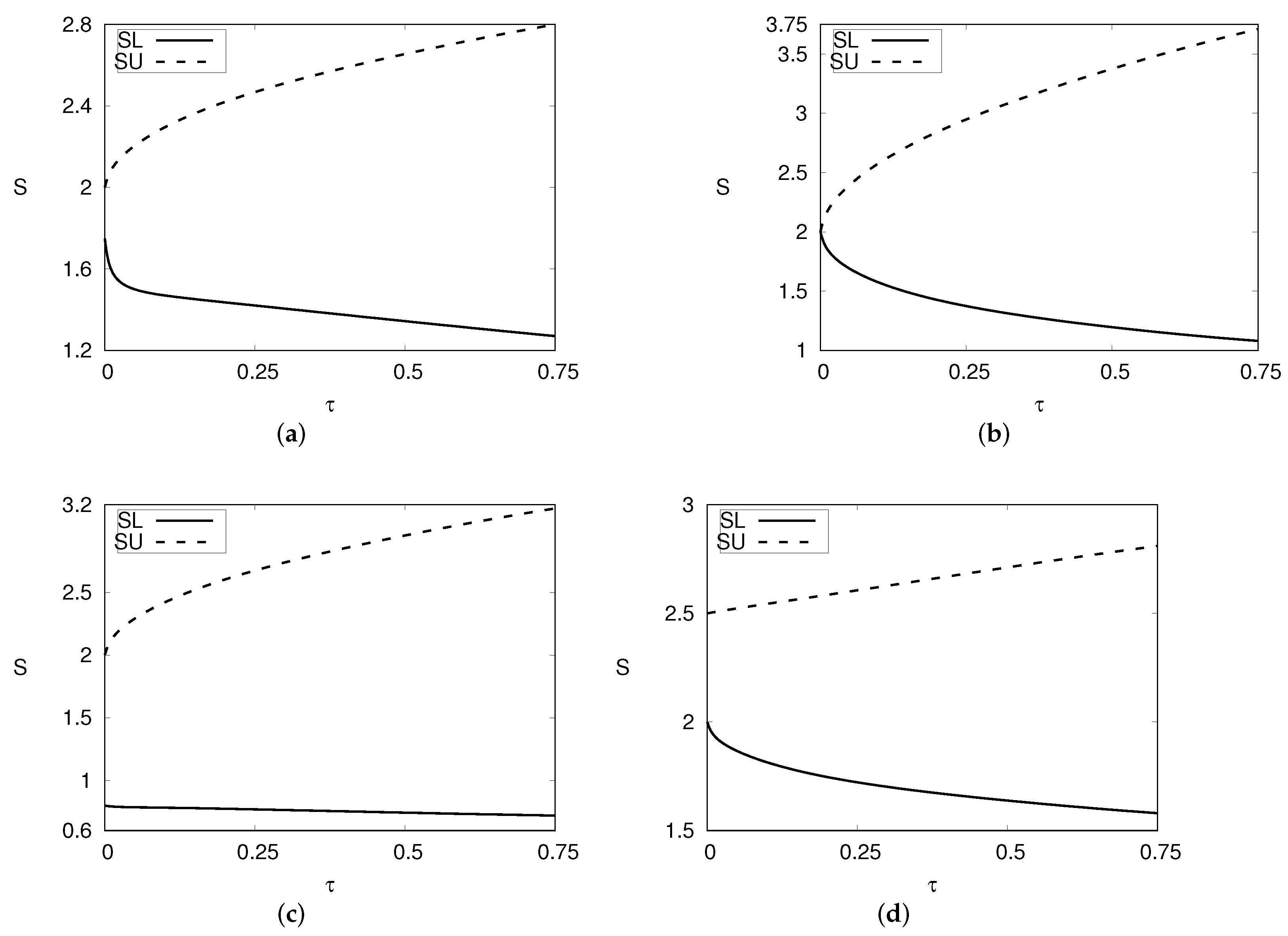
Plots of optimal exercise boundaries, $S_l$ and $S_u$ for $0\le \tau \le \frac{9}{12}$ calculated using Theorem 1 are given in Figure 2 using $X=2$ and a variety of parameter values for $\sigma ,r$ and q. From the figures it can be seen that at $\tau =0$, when $r>q$ that $S_u=rX/q$ and $S_l=X$; when $r<q$ that $S_u=X$ and $S_l=Xr/q$ and when $r=q$, $S_u=S_l=X=2$. This is in agreement with the results of Qiu [10]. From $\tau =0,$$S_u$ increases, (at first more sharply) while $S_l$ decreases with $\tau$.

3. Early Exercise Price at Small Maturities

Recall that in the previous section we defined $\theta =\frac{x}{\sigma \sqrt{\tau }}$ where $x=ln\left(\frac{X}{S}\right)$. In this section, we demonstrate how our representation of the solution when $r>q$ leads to an approximation ${\widehat{\theta }}_2$ of the early exercise level for the lower boundary $S_l$ in (11) as $\tau$ tends to 0 which is similar to asymptotic results found in the literature for the free boundary in American put options (see, e.g., Lamberton Villeneuve [12] and Kwok [1]). However, when $r=q$ the behavior differs from that of the American put free boundary as $\tau$ tends to zero. For the upper boundary, the behaviors are interchanged.

Proposition 1.

When $r>q$, the solution (5) leads to an approximation ${\widehat{\theta }}_2$ of the early exercise level in (11) that is $\sim \sqrt{ln(1/\tau )}$ as τ tends to 0 and when $r=q$ behaves like ${\displaystyle \sqrt{W_L\left(\frac{1}{{\tau }^2}\right)}}$, where $W_L$ is the Lambert function which satisfies $W_L\left(x\right)e^{W_L\left(x\right)}=x$.

Proof. 

We have in $0\le \theta \le z$, $\begin{array}{ccc}\hfill V(\theta ,\tau ;y,z)& =& e^{-q\tau }{e}^{A\sigma \sqrt{\tau }\theta }{e}^{B\tau }{e}^{-{\theta }^2/2}[\sqrt{\tau }\left\{(C_1+4D_1)M\left(1,\frac{1}{2},\frac{{\theta }^2}{2}\right)-D_{1}U\left(1,\frac{1}{2},\frac{{\theta }^2}{2}\right)\right\}\hfill \\ & +& R(\theta ,\tau ;y,z)\tau ],\hfill \end{array}$ where

$${\displaystyle R(\theta ,\tau ;y,z)=\sum _{i=2}^{\infty }{\tau }^{\frac{i-2}{2}}\left[\left(C_i+\frac{2D_i\sqrt{\pi }}{\mathsf{\Gamma }(1+i/2)}\right)M\left(\frac{1+i}{2},\frac{1}{2},\frac{{\theta }^2}{2}\right)-D_{i}U\left(\frac{1+i}{2},\frac{1}{2},\frac{{\theta }^2}{2}\right)\right].}$$

From (13), we have that for small $\tau$, $V_z({\tilde{\theta }}_2,\tau ;\infty ,{\tilde{\theta }}_2)=0$. This leads to

$$\begin{array}{ccc}& & \sqrt{\tau }\left\{{(C_1+4D_1)}_{z}M\left(1,\frac{1}{2},\frac{{\widehat{\theta }}_2^2}{2}\right)-{\left(D_1\right)}_{z}U\left(1,\frac{1}{2},\frac{{\widehat{\theta }}_2^2}{2}\right)\right\}+R_z({\widehat{\theta }}_2,\tau ;\infty ,{\widehat{\theta }}_2)\tau =0\hfill \\ & & {\displaystyle \Rightarrow \frac{2X\sigma }{e^{\frac{-{\widehat{\theta }}_2^2}{2}}+{\widehat{\theta }}_2\sqrt{\frac{\pi }{2}}[1+erf\left(\frac{{\widehat{\theta }}_2}{\sqrt{2}}\right)]}+R_z\sqrt{\tau }=0.}\hfill \end{array}$$

(30)

Now, using the relation that for large z

$$erf\left(\frac{z}{\sqrt{2}}\right)\sim 1-\frac{2}{z\sqrt{2\pi }}{e}^{-z^2/2}$$

(31)

we get

$${\displaystyle \frac{2X\sigma }{{\widehat{\theta }}_2\sqrt{2\pi }}\sim -R_z\sqrt{\tau }.}$$

(32)

We now examine the leading order term of $R_z$ when $r>q,$ which is

$${(C_2+2\sqrt{\pi }{D}_2)}_{z}M\left(\frac{3}{2},\frac{1}{2},\frac{{\theta }^2}{2}\right)-{\left(D_2\right)}_{z}U\left(\frac{3}{2},\frac{1}{2},\frac{{\theta }^2}{2}\right).$$

(33)

Using (31) the leading order behavior is found to be ${\displaystyle \sim \frac{8X(q-r)e^{{\widehat{\theta }}_2^2/2}{\widehat{\theta }}_2^3}{4{\widehat{\theta }}_2^4}.}$

Hence, from (32) we have

$${\displaystyle \frac{2\sigma }{{\widehat{\theta }}_2\sqrt{2\pi }}\sim -\frac{8(q-r)e^{{\widehat{\theta }}_2^2/2}}{4{\widehat{\theta }}_2}\sqrt{\tau }.}$$

(34)

This makes sense only if $r>q$ and so for this case we get on rearranging (34) ${\widehat{\theta }}_2\sim \sqrt{ln(1/\tau )}.$

When $r=q$ then for the leading order behavior of $R_z$ we go to

$${(C_3+\frac{8D_3}{3})}_{z}M\left(2,\frac{1}{2},\frac{{\theta }^2}{2}\right)-{\left(D_3\right)}_{z}U\left(2,\frac{1}{2},\frac{{\theta }^2}{2}\right).$$

(35)

Using (31) we get the leading order behavior $\sim -2r\sigma X{e}^{{\widehat{\theta }}_2^2/2}$.

Hence, we have

$${\displaystyle \frac{2\sigma }{{\widehat{\theta }}_2\sqrt{2\pi }}\sim 2r\sigma e^{{\widehat{\theta }}_2^2/2}\tau .}$$

(36)

From this, we get

$$\begin{array}{c}\hfill {\widehat{\theta }}_2{e}^{{\widehat{\theta }}_2^2/2}\sim \frac{1}{\tau }\mathrm{so}\mathrm{that}{\widehat{\theta }}_2^2{e}^{{\widehat{\theta }}_2^2}\sim \frac{1}{{\tau }^2}.\end{array}$$

Hence, ${\widehat{\theta }}_2\sim \sqrt{W_L\left({\tau }^{-2}\right)}$ where $W_L$ is the Lambert function (see Abramowitz and Stegun [15]). □

Remark 1.

When $r<q$ the right hand side of (34) would be negative and thus the above analysis fails. In this case, we cannot use the leading order of $R_z$ as in (33) even though the terms in $R_z$ eventually go to zero. It is believed that in this case ${\widehat{\theta }}_2\sim 1/\sqrt{\tau },$ by comparing (11) and the known behavior at expiry of American put options $S_f\left(T\right)=X\frac{r}{q}$ when $r<q$ (see, e.g., Kwok [1]), which is evidenced in our solutions.

Proposition 2.

Solution (5) leads to an approximation $Y=-{\widehat{\theta }}_1>0$ of the early exercise level in (10) that is $\sim \sqrt{ln(1/\tau )}$ as τ tends to 0 when $r<q$ and when $r=q$ behaves like ${\displaystyle \sqrt{W_L\left(\frac{1}{{\tau }^2}\right)}}$, where $W_L$ is the Lambert function which satisfies $W_L\left(x\right)e^{W_l\left(x\right)}=x$.

Proof. 

The proof for this proposition is similar to that for Proposition 4.1. We have in $-y\le \theta \le 0$

$$V(\theta ,\tau ;y,z)=e^{-q\tau }{e}^{A\sigma \sqrt{\tau }\theta }{e}^{B\tau }{e}^{-{\theta }^2/2}\left[\sqrt{\tau }\left\{C_{1}M\left(1,\frac{1}{2},\frac{{\theta }^2}{2}\right)+D_{1}U\left(1,\frac{1}{2},\frac{{\theta }^2}{2}\right)\right\}+R(\theta ,\tau ;y,z)\tau \right],$$

where

$${\displaystyle R(\theta ,\tau ;y,z)=\sum _{i=2}^{\infty }{\tau }^{\frac{i-2}{2}}\left[C_{i}M\left(\frac{1+i}{2},\frac{1}{2},\frac{{\theta }^2}{2}\right)+D_{i}U\left(\frac{1+i}{2},\frac{1}{2},\frac{{\theta }^2}{2}\right)\right].}$$

From (12) we have that $V_y(Y,\tau ;Y,\infty )=0$. This leads to

$$\begin{array}{ccc}& & \sqrt{\tau }\left\{{\left(C_1\right)}_{y}M\left(1,\frac{1}{2},\frac{Y^2}{2}\right)+{\left(D_1\right)}_{y}U\left(1,\frac{1}{2},\frac{Y^2}{2}\right)\right\}+R_y(Y,\tau ;Y,\infty )\tau =0.\hfill \end{array}$$

(37)

Using the relation for large y as given in (31) we get

$${\displaystyle \frac{2X\sigma }{Y\sqrt{2\pi }}\sim -R_y\sqrt{\tau }.}$$

(38)

We now look at the leading order term of $R_y$, namely

$$\left[{\left(C_2\right)}_{y}M\left(\frac{1+i}{2},\frac{1}{2},\frac{{\theta }^2}{2}\right)+{\left(D_2\right)}_{y}U\left(\frac{1+i}{2},\frac{1}{2},\frac{{\theta }^2}{2}\right)\right].$$

(39)

Using (31) we get the leading order behavior

$$\sim -\frac{2e^{Y^2/2}(q-r)}{Y},$$

(40)

so that using (38) and (40) we get

$$\frac{2\sigma }{Y\sqrt{2\pi }}\sim \frac{2e^{Y^2/2}(q-r)}{Y}\sqrt{\tau }.$$

(41)

This only makes sense if $q>r$ in which case $e^{-Y^2/2}\sim \sqrt{\tau }$ so that $Y\sim \sqrt{ln(1/\tau )}.$

When $r=q$ then the leading order behavior of $R_y$ is

$${\left(C_3\right)}_{y}M\left(2,\frac{1}{2},\frac{{\theta }^2}{2}\right)+{\left(D_3\right)}_{y}U\left(2,\frac{1}{2},\frac{{\theta }^2}{2}\right).$$

(42)

Using (31) and (42) we get the leading order behavior of $R_y$$\sim -2Xr\sigma e^{Y^2/2}$.

Hence, from (38) (but with the RHS now $-R_y\tau$) we have

$${\displaystyle \frac{2\sigma }{Y\sqrt{2\pi }}\sim 2r\sigma e^{Y^2/2}\tau .}$$

(43)

From this, we get

$$e^{Y^2}{Y}^2\sim \frac{1}{{\tau }^2}.$$

(44)

Hence $Y\sim \sqrt{W_L\left({\tau }^{-2}\right)}.$ □

We now make a similar remark as for the previous proposition.

Remark 2.

When $r>q$ the right hand side of (41) would be negative and thus the above analysis fails. So for $r>q$ we are unable to use the leading order of $R_y$ as in (42), however the terms in $R_y$ eventually go to zero. By comparing (10) and the known behavior at expiry of American call options $S_f\left(T\right)=X\frac{r}{q}$ when $r>q$ (see, e.g., Kwok [1]), it is presumed that in this case ${\widehat{\theta }}_1\sim 1/\sqrt{\tau }.$ This is supported by our solutions.

4. Some Comparisons with a Numerical Method

We now assess the performance of the formula in Theorem 1 (T1) for pricing American straddle options up to 9 months maturity with that obtained numerically using (2), (3a)–(3e). The solution method in this paper is designed for American straddles with a short time to maturity, e.g., up to 1 year, as the majority of American options have a lifespan of less than 9 months. The numerical method we used was the Crank–Nicolson (CN) method with successive over-relaxation which is accurate to $O(d{t}^2,d{S}^2)$ (see Wilmott [16]) where $dt$ and $dS$ are the increments in time and asset price respectively (note that the increment sizes $dt$ and $dS$ obviously affect the speed and accuracy of the CN scheme. If the largest S value in the grid is denoted $S_{max}$ then the number of S intervals is $M=\frac{S_{max}}{dS}$ and the size of the coefficient matrices are $(M-1)\times (M-1)$. Here, we used $S_{max}=7$ and chose increments so that when halved, did not alter the solution to 4 decimal places. Typically, this was $dS={10}^{-2}$ and $dt=0.5\times {10}^{-3}$ or $0.25\times {10}^{-3}$).

In

Table 1. Comparison of American straddle option prices with $X=2$ using Theorem 1 (T1) and the Crank–Nicolson scheme (CN).

$(\mathit{\sigma },\mathit{r},\mathit{q})$	S	$\mathit{\tau }=1/12$		$\mathit{\tau }=2/12$		$\mathit{\tau }=3/12$		$\mathit{\tau }=6/12$		$\mathit{\tau }=9/12$
		CN	T1	CN	T1	CN	T1	CN	T1	CN	T1
(0.2,0.03,0.04)	1.8	0.2038	0.2038	0.2157	0.2157	0.2299	0.2299	0.2716	0.2715	0.3084	0.3082
	1.9	0.1237	0.1237	0.1519	0.1519	0.1760	0.1760	0.2333	0.2333	0.2780	0.2779
	2.0	0.0919	0.09191	0.1297	0.1297	0.1585	0.1585	0.2226	0.2225	0.2707	0.2706
	2.1	0.1252	0.1252	0.1548	0.1548	0.1799	0.1799	0.2395	0.2395	0.2859	0.2859
	2.2	0.2037	0.2037	0.2179	0.2179	0.2344	0.2343	0.2812	0.2812	0.3218	0.3217
(0.3,0.02,0.02)	1.8	0.2175	0.2175	0.2495	0.2495	0.2797	0.2797	0.3567	0.3567	0.4192	0.4192
	1.9	0.1574	0.1574	0.2063	0.2063	0.2456	0.2456	0.3361	0.3361	0.4057	0.4057
	2.0	0.1379	0.1380	0.1947	0.1947	0.2381	0.2381	0.3350	0.3350	0.4082	0.4082
	2.1	0.1632	0.1633	0.2152	0.2152	0.2568	0.2568	0.3524	0.3524	0.4258	0.4258
	2.2	0.2246	0.2246	0.2634	0.2634	0.2988	0.2988	0.3866	0.3866	0.4571	0.4571
(0.3,0.02,0.05)	1.8	0.2209	0.2209	0.2546	0.2546	0.2862	0.2862	0.3656	0.3656	0.4296	0.4295
	1.9	0.1595	0.1595	0.2092	0.2092	0.2491	0.2491	0.3408	0.3408	0.4110	0.4109
	2.0	0.1380	0.1381	0.1949	0.1950	0.2383	0.2383	0.3352	0.3351	0.4081	0.4080
	2.1	0.1615	0.1615	0.2128	0.2128	0.2539	0.2538	0.3481	0.3480	0.4202	0.4201
	2.2	0.2219	0.2219	0.2590	0.2590	0.2931	0.2931	0.3783	0.3782	0.4467	0.4465
(0.2,0.02,0.01)	1.8	0.2020	0.2020	0.2124	0.2124	0.2256	0.2256	0.2659	0.2659	0.3022	0.3022
	1.9	0.1222	0.1222	0.14980	0.1498	0.1736	0.1736	0.2309	0.2309	0.2763	0.2763
	2.0	0.0920	0.0920	0.1301	0.1301	0.1592	0.1592	0.2246	0.2246	0.2743	0.2743
	2.1	0.1271	0.1271	0.1578	0.1579	0.1839	0.1840	0.2461	0.2461	0.2951	0.2951
	2.2	0.2063	0.2063	0.2226	0.2227	0.2408	0.2408	0.2918	0.2918	0.3359	0.3359
RMSE		$3.9\times {10}^{-5}$		$3.2\times {10}^{-5}$		$3.9\times {10}^{-5}$		$5.0\times {10}^{-5}$		$9.5\times {10}^{-5}$

we compare American straddle prices V using Theorem 1 (T1) with that obtained using the CN method. We used $X=2$ and a variety of other parameter values for $\sigma ,r,q$ and S and with maturity times from 1 to 9 months. As can be seen from the table, the price solutions agree remarkably well with mostly 4 decimal place accuracy and with root mean square errors (RMSEs) for all the maturities being less than ${10}^{-4}$.

In

Table 2. Comparison of optimal exercise stock prices ($S_u,$ the upper price and $S_l,$ the lower price) with $X=2$ using Theorem 1 (1) and the Crank–Nicolson scheme (CN).

$(\mathit{\sigma },\mathit{r},\mathit{q})$	${\mathit{S}}_{\mathit{value}}$	$\mathit{\tau }=1/12$		$\mathit{\tau }=2/12$		$\mathit{\tau }=3/12$		$\mathit{\tau }=6/12$		$\mathit{\tau }=9/12$
		CN	T1	CN	T1	CN	T1	CN	T1	CN	T1
(0.2,0.03,0.04)	$S_u$	2.31	2.31	2.42	2.42	2.50	2.50	2.68	2.67	2.80	2.80
	$S_l$	1.46	1.47	1.44	1.45	1.41	1.42	1.33	1.34	1.26	1.27
(0.3,0.02,0.02)	$S_u$	2.60	2.61	2.82	2.83	3.00	3.00	3.41	3.42	3.71	3.71
	$S_l$	1.54	1.54	1.41	1.41	1.33	1.33	1.17	1.17	1.08	1.08
(0.3,0.02,0.05)	$S_u$	2.44	2.44	2.60	2.60	2.72	2.72	2.98	2.98	3.18	3.17
	$S_l$	0.79	0.79	0.78	0.78	0.77	0.77	0.73	0.74	0.71	0.72
(0.15,0.05,0.04)	$S_u$	2.55	2.54	2.58	2.57	2.61	2.60	2.72	2.72	2.81	2.81
	$S_l$	1.8	1.8	1.74	1.74	1.70	1.70	1.62	1.63	1.57	1.58
RMSE		$6.1\times {10}^{-3}$		$6.1\times {10}^{-3}$		$5.0\times {10}^{-3}$		$7.9\times {10}^{-3}$		$7.1\times {10}^{-3}$

, we compare the upper and lower optimal exercise boundaries obtained using (12) and (13) with that obtained numerically. The values agree extremely well in all cases. Hence, the solution as described in Theorem 1 has shown to be remarkably accurate not just for the option values, but also for the OEBs values.

As a further test, we compared the computational times for the Crank–Nicolson numerical method with that of the proposed solution in this paper. Using the computer algebra package Maple [17] on a Dell x64 PC, (Intel Core i7 processor, 16 GB RAM, CPU @3.6 GHz) we found that using $n=4$ terms in the series expansions for the American straddle price, the new solution presented in this paper took under one and a half seconds in real time or under one second in CPU time, to yield the straddle price. Using $n=10$ terms took about 3 s in real time or 2.56 s in CPU time. In comparison, the numerical CN method could take between 25 and 300 s depending on the time to maturity, or between 86 and 1000 s CPU time. Given that fast and accurate answers are critical in practice, this is an important development in the area of option pricing.

5. Conclusions

There are currently close to 5 million options listed on the Chicago Board of Exchange (CBOE) (see https://markets.cboe.com/, accessed on 21 April 2022) with over 376 million open interest. The overwhelming majority of these options have less than 9 months to maturity. Hence, with short-tenor American options, whether they be vanilla or exotic, being in such demand, it is no surprise that the matter of pricing these options is so useful and crucial. In this paper, we have provided a very accurate and efficient analytical approximation for American straddle options with short-tenor in the form of a series solution; the coefficients of which are in terms of standard mathematical functions. As such, solutions of all orders can be found extremely swiftly. We have also demonstrated that the solution provides very accurate results. While some analytic approximations proposed in the literature might yield good results in some cases for either the option price or the critical stock price, remarkably our solution provides very accurate results for both for the option price and for the critical stock prices. This is a highlight of the solution method as many analytic approximations to American options yield either good option prices or critical stock prices, but not both. We have also examined the behavior of the critical boundaries near expiry and found they were dependent on the relative values of the risk-free interest rate r and the dividend yield q. Like American put options, when $r>q$, the lower boundary of the American straddle tends to the strike price, X, in the parabolic-logarithmic form, and when $r<q$, the upper boundary of the American straddle behaves like the free boundary of American call options and tends to the strike price in the parabolic-logarithmic form. However, when $r=q$, the behaviors differ from their American vanilla counterparts. In the case $r<q$ for the lower boundary and $r>q$ for the upper boundary, we surmised and observed they tended towards $Xr/q$ parabolically as time to expiry tended towards zero.

References

1. Kwok, Y. Mathematical Models of Financial Derivatives; Springer: Singapore, 1998. [Google Scholar]
2. Alobaidi, G.; Mallier, R. Laplace transforms and the American straddle. J. Appl. Math. 2002, 3, 121–129. [Google Scholar] [CrossRef] [Green Version]
3. Alobaidi, G.; Mallier, R. The American straddle close to expiry. Bound. Value Probl. 2006, 2006, 32835. [Google Scholar] [CrossRef] [Green Version]
4. Kim, I. The analytic valuation of American options. Rev. Financ. Stud. 1990, 3, 547–572. [Google Scholar] [CrossRef]
5. Chiarella, C.; Ziogas, A. Evaluation of American strangles. J. Econ. Dyn. Control 2005, 3, 31–62. [Google Scholar] [CrossRef] [Green Version]
6. Detemple, J. American-Style Derivatives: Valuation and Computation; Chapman & Hall/CRC: Boca Raton, FL, USA, 2006. [Google Scholar]
7. Gao, X.; Deng, D.; Shan, Y. Lattice methods for pricing American strangles with two-dimensional stochastic volatility models. Discrete Dyn. Nat. Soc. 2014, 1, 1–6. [Google Scholar] [CrossRef]
8. Kang, M.; Jeon, J.; Han, H.; Lee, S. Analytic solution for American strangle options using Laplace–Carson transforms. Commun. Nonlinear Sci. Numer. Simul. 2017, 47, 292–307. [Google Scholar] [CrossRef]
9. Ma, J.; Li, W.; Cui, Z. Valuation of American Strangles Through an Optimized Lower–Upper Bound Approach. J. Oper. Res. Soc. China 2018, 6, 25–47. [Google Scholar] [CrossRef]
10. Qiu, S. American Strangle options. Appl. Math. Financ. 2020, 7, 228–263. [Google Scholar] [CrossRef]
11. Medvedev, A.; Scaillet, O. Pricing American options under stochastic volatility and stochastic interest rates. J. Financ. Econ. 2010, 98, 145–159. [Google Scholar] [CrossRef] [Green Version]
12. Lamberton, D.; Villeneuve, S. Critical price near maturity for an American option on a dividend-paying stock. Ann. Appl. Probab. 2003, 13, 800–815. [Google Scholar] [CrossRef]
13. Covei, D. On a parabolic partial di¤erential equation and system modeling a production planning problem. Electron. Res. Arch. 2022, 30, 1340–1453. [Google Scholar] [CrossRef]
14. Tao, L. On free boundary problems with arbitrary initial and flux conditions. J. Appl. Math. Phys. 1979, 30, 416–426. [Google Scholar] [CrossRef]
15. Abramowitz, M.; Stegun, I. Handbook of Mathematical Functions With Formulas, Graphs, and Mathematical Tables; U.S. Government Publishing Office: Washington, DC, USA, 1998.
16. Wilmott, P. Derivatives: The Theory and Practice of Financial Engineering; John Wiley & Sons: Chichester, UK, 1998. [Google Scholar]
17. Maple. Maplesoft; A Division of Waterloo Maple Inc.: Waterloo, ON, Canada, 2018. [Google Scholar]
Figure 1. American straddle prices with parameters X = 2 , σ = 0.2 , r = 0.03 , q = 0.04 for τ = 1 / 12 and τ = 9 / 12 .
Mathematics 10 01401 g001
Figure 2. Optimal exercise stock prices for 0 τ 9 12 using X = 2 and (a) σ = 0.2 , r = 0.03 , q = 0.04 , (b) σ = 0.3 , r = 0.02 , q = 0.02 , (c) σ = 0.3 , r = 0.02 , q = 0.05 and (d) σ = 0.15 , r = 0.05 , q = 0.04 .
Mathematics 10 01401 g002