Article

Observer-Based PID Control Strategy for the Stabilization of Delayed High Order Systems with up to Three Unstable Poles

by
César Cruz-Díaz
1,
Basilio del Muro-Cuéllar
1,*,
Gonzalo Duchén-Sánchez
1,
Juan Francisco Márquez-Rubio
1 and
Martín Velasco-Villa
2
1
Instituto Politécnico Nacional, ESIME Culhuacán, Av. Santa Ana 1000, Col. San Francisco Culhuacán, Mexico City 04440, Mexico
2
Centro de Investigación y de Estudios Avanzados del Instituto Politécnico Nacional, Electrical Engineering Department, Mechatronics Section, Av. IPN 2508, Col. San Pedro Zacatenco, Mexico City 07360, Mexico
*
Author to whom correspondence should be addressed.
Mathematics 2022, 10(9), 1399; https://doi.org/10.3390/math10091399
Submission received: 24 March 2022 / Revised: 18 April 2022 / Accepted: 19 April 2022 / Published: 22 April 2022

Abstract

:
In this paper, a new method to manage the stabilization and control problems of n-dimensional linear systems plus dead time, which includes one, two, or three unstable poles, is proposed. The control methodology proposed in this work is an Observer-based Proportional-Integral-Derivative (PID) strategy, where an observer and a PID controller are used to relocate the original unstable open-loop poles to stabilize the resultant closed-loop system. The observer provides an adequate estimation of the delayed-free variables and the PID uses the delay-free variables estimated by the proposed observer. Also, step-tracking is achieved in the overall control scheme. Necessary and sufficient conditions are presented to ensure closed-loop stability based on the open loop parameters of the system. The observer-based PID strategy considers five to seven constant parameters to obtain a stable closed-loop system. A general procedure to implement the proposed control strategy is presented and its performance is evaluated by means of numerical simulations.
MSC:
93C43; 93B53; 93C05; 93Dxx

1. Introduction

A dynamical system may be characterized by the existing relationship between its input and output signals. In any dynamical system, the appearance of a change in the output and its detection at the input to make a decision always occurs after a finite period of time. This period is called time delay or simply delay. When the size of the delay is not significant compared to the characteristics of the system, that is, with the dominant time constant, the analysis and control of such systems are not difficult to carry out, and the time delay can even be neglected. Conversely, when the magnitude of the delay approaches or exceeds the system time constant value, other techniques are necessary to design controllers that mitigate its effect. In general, time delay is an intrinsic attribute of several dynamical systems like financial systems [1], biological systems [2], chemical processes [3], thermal systems [4], tele-operation systems [5], mechanical systems [6], communications systems [7], electrical systems [8], hydraulic actuators [9], robotic systems [10], and many others [11]. Nevertheless, necessary and sufficient conditions to stabilize such systems have only been given for particular cases and several problems remain open, in particular, the case of observer-based controllers for delayed high order systems.
Observer-based strategies for systems with time-varying delays, or delays on input and output signals, still constitute open problems. The strategy commonly taken to handle with delayed systems is mainly based on the classic Smith predictor [12], which is a method that tries to counteract the effect of the time delay using strategies to estimate the future value of the output signal on the design of a control feedback. This approach has the disadvantage of being restricted to open loop stable systems. Some modifications to the original Smith predictor for the case of unstable systems can be consulted in Refs. [13,14], also a few recent papers have been published using this approach [15].
Another approach to stabilize unstable systems with delay is the consideration of P, PI, PD, and PID control actions. In Ref. [16], the results for the stabilization of a delayed system with a single unstable real pole and several stable real poles using classical controllers are presented, while in Ref. [17] the stabilization of the same systems with possible complex conjugate stable poles is considered. It is worth mentioning that it is not possible to stabilize delayed systems with more than two unstable poles using a P, P I controller [18].
The observer-based control of high order systems with one or two unstable poles is discussed in Refs. [19,20]. In Ref. [19], the stability of linear delayed systems with two unstable real poles using an observer-based scheme is studied, a robustness analysis is presented, and a two degree of freedom PI control action is implemented to track step references and reject disturbances. In Ref. [20], the stabilization and control of linear delayed systems with two unstable real poles and n stable real poles using an Observer- P I scheme is considered, and the control scheme manages the problem of regulation and step disturbance rejection.
In Ref. [21], the stabilization and control of delayed systems containing minimum phase zeros is analyzed, sufficient conditions are provided with the objective to guarantee the stabilization of high-order delayed systems including m real left half-plane (LHP) zeros, by using proportional, derivative and integral controllers.
In Ref. [22], the case of high order systems with two unstable poles and and several real stable poles using a P D -observer scheme is presented. This proposal is extended in [23] by considering the case of complex conjugated stable poles. In particular, in [23] an observer scheme is proposed including a Proportional Derivative P D controller to stabilize systems with two unstable poles and several stable poles, the latter being able to be complex conjugates. The work [23] improves the result mentioned in Ref. [22], by increasing the size of the admissible delay in the plant and taking into account the possibility of conjugated complex poles in the plant.
In the literature, several strategies considering the use of observers have been applied to delayed systems, for instance [19], in this work, an observer-based controller is presented to achieve the stabilization and control of linear time invariant high order delayed systems with two unstable real poles. In [24], an infinite dimensional observer with an adaptive time delay estimation and a sliding mode controller is proposed.
Up to the best of our knowledge, the necessary and sufficient condition for the stabilization of high order delayed systems with three unstable poles has not been addressed in the literature. Motivated by this consideration, in this paper, a novel general scheme is proposed for the stabilization of delayed high order systems with one, two, and even three unstable poles. The main contributions of this paper can be summarized as follows: First, the ability to stabilize systems with three unstable poles. Second, the generalization of being able to also stabilize systems with one and two unstable poles. Third, the admissible delay is increased compared to previously presented strategies. Numerical examples illustrate the effectiveness of the proposed scheme.
The remainder of this paper is organized as follows. In Section 2, the problem statement is given, and some preliminary results already presented in the literature are provided. In Section 3, the main results of the work are presented. In Section 4, a numerical evaluation of the proposed strategy through some academic examples is given. Finally, the general conclusions of the work are stated in Section 5.

2. Problem Statement

It is considered a class of unstable delayed single-input single-output (SISO) linear systems with time-delay in the direct path. Furthermore, it is assumed that the system has one, two, or three unstable poles. The system is given by the transfer function,
Y ( s ) U ( s ) = G u j ( s ) G s ( s ) e τ s
where Y ( s ) is the output signal, U ( s ) the input signal, G u j ( s ) is an unstable transfer function with j = 1 , 2 , 3 unstable poles, G s ( s ) is a stable subsystem with n j poles and τ > 0 is the magnitude of dead time. In particular, the subsystem G u j ( s ) can be defined as one of the following transfer functions,
G u j ( s ) = i = 1 j G α i ( s ) for j = 1 , 2 , 3
where
G α i ( s ) = 1 ( s α i )
with α i R + , and without loss of generality, it will be assumed that α 3 α 2 α 1 .
The stable subsystem G s ( s ) , is defined as,
G s ( s ) = ρ i = 1 n j ( s + β i )
where β i , i = 1 , , n j are real positive constants.
A PID control is defined as,
C P I D ( s ) = k p + k i s + k d s
where k p , k i and k d are the proportional, integral, and derivative positive constant gains, respectively.
The main objective of this work is to propose an observer (predictor) based controller, including a PID action, in order to stabilize the system with up to three unstable poles, which could be difficult, for the cases of one or two unstable poles, and not possible for the case of three unstable poles with the direct use of a PID controller [25].

Preliminary Results

For the sake of completeness and well understanding of the main results, this section presents some preliminary results already presented in the literature.
Consider first the unstable transfer function (1) for the case j = 1 , that is,
Y ( s ) U ( s ) = 1 ( s α 1 ) G s ( s ) e τ s .
Lemma 1
([16]). The unstable delayed system (6) can be stabilized by means of the proportional feedback,
U ( s ) = K [ R ( s ) Y ( s ) ]
where R ( s ) is the new input reference and K R , if and only if,
τ < 1 α 1 i = 1 n 1 1 β i .
Lemma 2
([16]). The delayed unstable system (6) can be stabilized by means of the PID controller given by (5), and the feedback,
U ( s ) = C P I D ( s ) [ R ( s ) Y ( s ) ]
if and only if,
τ < 2 α 1 i = 1 n 1 2 β i .
Remark 1.
Note that system (6) with G s ( s ) = 1 , can be stabilized by means of a proportional feedback if and only if τ < 1 α 1 . The same system, can be stabilized by using a PID controller under the necessary and sufficient condition τ < 2 α 1 .
For the case of two unstable poles j = 2 , Equation (1) takes the form,
Y ( s ) U ( s ) = 1 ( s α 1 ) ( s α 2 ) G s ( s ) e τ s .
Lemma 3
([25]). The unstable delayed system (10) can be stabilized by means of the PID controller (9), if and only if,
τ < 1 α 1 + 1 α 2 i = 1 n 2 1 β i 1 α 1 2 + 1 α 2 2 + i = 1 n 2 1 β i 2 .
Remark 2.
Note that system (10) with G s ( s ) = 1 , can be stabilized by means of the PID controller (9), if and only if,
τ < 1 α 1 + 1 α 2 1 α 1 2 + 1 α 2 2 .

3. Main Results

In this section, the case of linear systems with delay and three unstable poles is presented. First of all, the case of three unstable poles is analyzed considering an ideal case where all the internal variables are available for measurement. To overcome this ideal problem, the proposed observer is presented, and the corresponding closed-loop system is analyzed, producing necessary and sufficient conditions. To end this section, the cases with one and two unstable poles are considered.

3.1. System with Three Unstable Poles

Consider the time-delay system (1) for the case of three unstable poles, i.e., j = 3 ,
Y ( s ) U ( s ) = G u 3 ( s ) G s ( s ) e τ s .

3.1.1. State Feedback Controller

In the case that all the states are available for measurement, the stabilization of system (13) by means of the PID controller (9) and the state feedback depicted in Figure 1 for a static gain F = f 1 f 2 f n 2 can be stated in the following lemma.
Lemma 4.
The system defined by (13) can be stabilized using the control strategy shown in Figure 1, if and only if,
τ < 1 α 2 + 1 α 3 1 α 2 2 + 1 α 3 2 .
Proof. 
Sufficiency. Consider the system (13) in closed-loop with the configuration shown in Figure 1 with F = f 1 f 2 f n 2 . Assume that (14) is satisfied and define δ i > 1 d i and γ i > 1 d i 2 ; for i = 1 , 2 , . . . , n 2 , with d 1 , . . . , d n 3 being the new closed-loop location of the i t h stable pole and d n 2 the new closed-loop location of the unstable pole α 1 . Consider now that δ i and γ i are small enough such that,
τ = 1 α 2 + 1 α 3 i = 1 n 2 δ i 1 α 2 2 + 1 α 3 2 + i = 1 n 2 γ i .
Then, it is easy to verify that,
τ < 1 α 2 + 1 α 3 i = 1 n 2 1 d i 1 α 2 2 + 1 α 3 2 + i = 1 n 2 1 d i 2 .
Noting that d i can be as large as desired, then by considering d i , the terms 1 d i can be neglected and from Remark 2, system (13) can be stabilized by the control strategy given in Figure 1.
Necessity. Consider the delayed system (13) with the control strategy shown in Figure 1, with the feedback parameters F = f 1 f 2 f n 2 and a controller C P I D ( s ) that ensure the stability of the overall system. The closed loop transfer function can be written as,
Y ( s ) E ( s ) = C P I D ( s ) ρ e τ s ( s α 2 ) ( s α 3 ) ( s + d 1 ) ( s + d 2 ) . . . ( s + d n 2 )
where d i , i = 1 , . . . , n 2 , are the new locations of the i t h poles.
From Lemma 3, system (17) with unitary feedback E ( s ) = R ( s ) Y ( s ) is stable if and only if,
τ < 1 α 2 + 1 α 3 1 α 2 2 + 1 α 3 2 + i = 1 n 2 1 d i 2 i = 1 n 2 1 d i
then, from Remark 2, it is possible to compute F such that d i , which allows to rewrite the previous condition as,
τ < 1 α 2 + 1 α 3 1 α 2 2 + 1 α 3 2 .

3.1.2. Auxiliary Output Injection Structure

Notice that the proposed control strategy in Figure 1, considers an ideal way to stabilize system (1) with j = 3 , but the variables used for the state feedback (through vector F ) can not be directly taken from the original system. This problem will be later overtaken by the design of an observer proposed to estimate the required variables for state feedback involved in the scheme of Figure 1.
Before presenting the observer-based control scheme for the case of three unstable poles system, the output injection structure shown in Figure 2 is analyzed. The result of this scheme will be used in the proof of the main result of the three unstable poles cases (in Section 3.1.3).
The following result deals with the closed-loop stability of system (13) with a feedback structure as proposed in the injection scheme given in Figure 2.
Lemma 5.
The closed-loop transfer function Y ¯ ( s ) U ¯ ( s ) obtained from the proposed injection strategy of Figure 2 is stable if and only if,
τ < 1 α 1 .
Proof. 
Sufficiency. Assume that τ < 1 α 1 holds and define μ > 1 c 2 + 1 c 3 > 0 , with c 2 and c 3 the new closed-loop location of the poles α 2 and α 3 under the effect of the output injection gains G = g 2 g 3 T given in Figure 2. First of all, consider that μ is small enough such that,
τ = 1 α 1 μ .
Then, for suitable values of c 2 and c 3 it is possible to write,
τ < 1 α 1 1 c 2 1 c 3 < 1 α 1 .
Since the unstable poles α 2 and α 3 were move to stable positions, there is only one unstable pole in the closed-loop system. From Remark 1, there exists a feedback of the form (7) with gain g 1 such that the closed-loop system is stable.
Necessity. Consider the delayed system (13) with the injection scheme given in Figure 2, such that the overall process is stable. The closed-loop transfer function of Y ¯ ( s ) W ¯ ( s ) can be written as,
Y ¯ ( s ) W ¯ ( s ) = g 1 e τ s ( s α 1 ) ( s + c 2 ) ( s + c 3 ) + g 1 e τ s .
From Lemma 1, the transfer function (23) is stable, if and only if,
τ < 1 α 1 1 c 2 1 c 3
then, from Remark 1, it is possible to consider d i , which allows to rewrite the previous condition as,
τ < 1 α 1 .

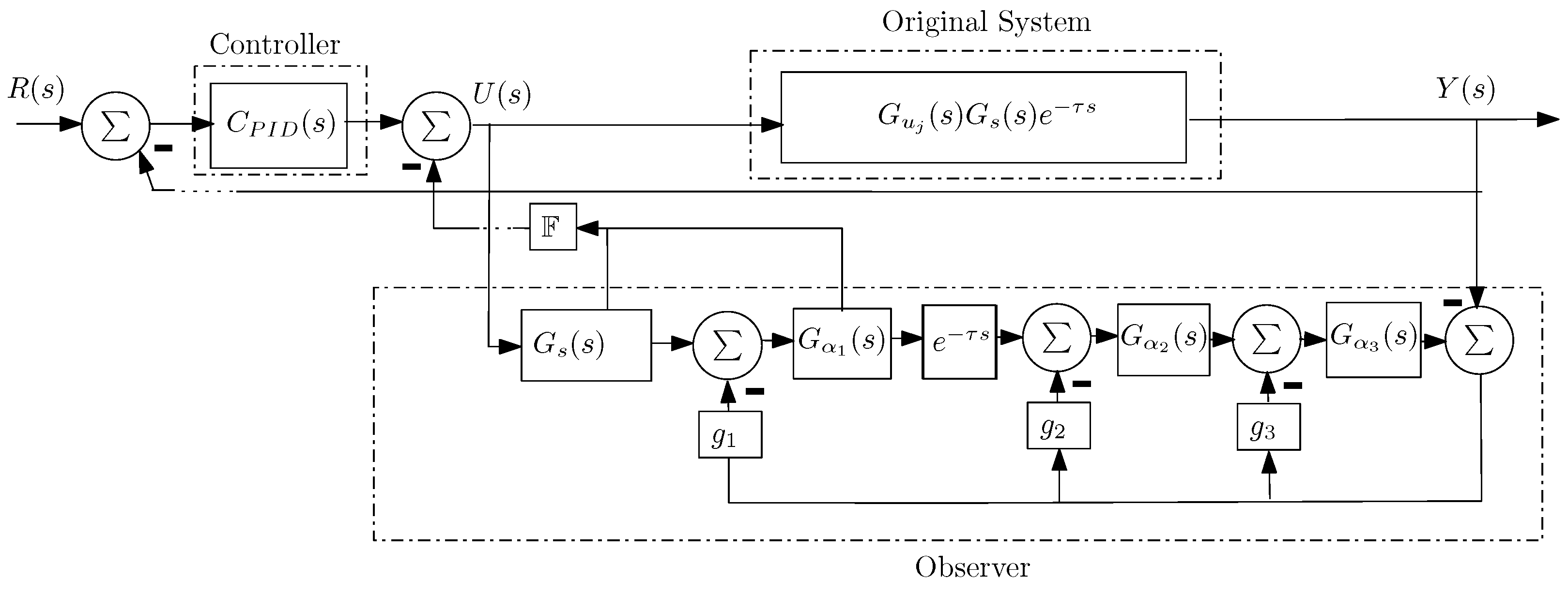
3.1.3. Observer-Based PID Control Scheme

The general observer-based PID control scheme for high order unstable time delay system with up to three unstable poles is depicted in Figure 3 where the feedback gains G = g 1 g 2 g 3 and F = f 1 f 2 f n 2 are considered.
It can be observed in Figure 3 how the control scheme shown in Figure 1 and the injection structure in Figure 2 are mixed to give the general control proposal. The next theorem gives the main result of the present work.
Theorem 1.
Consider the transfer function (13) where, without loss of generality, α 3 α 2 α 1 , together with the observer-based PID control scheme shown in Figure 3. Then, there exist gains G , F , k p , k i and k d such that the closed-loop system is stable, if and only if,
τ < m i n 1 α 1 , 1 α 2 + 1 α 3 1 α 2 2 + 1 α 3 2 .
Proof. 
A state space representation of the transfer function (13) is shown in Figure 4. Defining x ( t ) = x 1 ( t ) x 2 ( t ) x n 3 ( t ) z 1 ( t ) z 2 ( t ) z 3 ( t ) T it is possible to write,
x ˙ ( t ) = A 0 x ( t ) + A 1 x ( t τ ) + B u ( t ) y ( t ) = C x ( t )
where x i ( t ) , i = 1 , . . . , n 3 represent the stable subsystem; z j ( t ) , j = 1 , 2 , 3 are the unstable subsystem of the plant.
The parameters of system (27) are given by,
A 0 = β 1 0 0 0 0 0 0 0 1 β 2 0 0 0 0 0 0 0 1 β 3 0 0 0 0 0 0 0 0 β n 4 0 0 0 0 0 0 0 1 β n 3 0 0 0 0 0 0 0 1 α 1 0 0 0 0 0 0 0 0 α 2 0 0 0 0 0 0 0 1 α 3
A 1 = 0 0 0 0 0 0 0 0 0 0 0 0 0 0 0 0 0 0 0 0 0 0 0 0 0 0 0 0 0 0 0 0 1 0 0 0 0 0 0 0 0 0
B = ρ 0 0 0 0 0 T
C = 0 0 0 0 0 1 .
Note that the state space representation characterized by (27) can be rewritten in its transfer function representation by,
Y ( s ) U ( s ) = C ( s I ( A 0 + A 1 e τ s ) ) 1 B .
Also, from Figure 3, the dynamics of the proposed observer can be described as,
x ^ ˙ ( t ) = A 0 x ^ ( t ) + A 1 x ^ ( t τ ) + B u ( t ) G ( C x ^ ( t ) y ( t ) )
with
G ¯ = 0 0 0 g 1 g 2 g 3 T .
The estimation error e ( t ) = x ( t ) x ^ ( t ) produces,
e ˙ ( t ) = x ˙ ( t ) x ^ ˙ ( t ) = ( A 0 G ¯ C ) e ( t ) + A 1 e ( t τ ) .
Now, consider the control feedback u ( t ) = F ¯ x ^ ( t ) + k p ( r ( t ) y ( t ) ) + k i ( r ( t ) y ( t ) ) d t + k d d ( r ( t ) y ( t ) ) d t with
F ¯ = f 1 f 2 f n 2 0 0
produces the closed-loop system,
x ˙ ( t ) = A 0 x ( t ) + A 1 x ( t τ ) + B ( F ¯ x ^ ( t ) + k p ( r ( t ) y ( t ) ) + k i ( r ( t ) y ( t ) ) d t + k d d ( r ( t ) y ( t ) ) d t ) .
Considering the change of coordinates x e = x ( t ) e ( t ) T and after simple manipulations, the following closed-loop system is obtained:
x ˙ e ( t ) = A 0 B F ¯ B F ¯ 0 A 0 G ¯ C x e ( t ) + A 1 0 0 A 1 x e ( t τ ) + B ( k p ( r ( t ) y ( t ) ) + k i ( r ( t ) y ( t ) ) d t + k d d ( r ( t ) y ( t ) ) d t ) 0 y ( t ) = C 0 x e ( t ) .
The proposed observer-based controller satisfies the separation principle. From Lemma 4 (Figure 1) and Lemma 5 (Figure 2) it is easy to get a state space representation and verify that the stability of these two structures is equivalent to the stability in Equation (32). Hence, the stability of the proposed scheme is guaranteed if and only if the conditions in Lemma 4 and Lemma 5 are satisfied. Therefore, there exist gains G , F , k p , k i and k d such that the closed-loop system shown in Figure 3 is stable, if and only if,
τ < m i n 1 α 1 , 1 α 2 + 1 α 3 1 α 2 2 + 1 α 3 2 .

3.1.4. Controller Parameters Selection

The following guide is proposed to tune up the PID controller and to select the F and G parameters. Once the conditions of Theorem 1 are satisfied, we proceed as follows.
(a)
Consider Figure 1. For G s ( s ) G α 1 ( s ) we obtain a state space realization (matrices A and B), then chose F such that the eigenvalues of ( A B F ) become [ d 1 , d 2 , , d n 2 ] and relation (18) is satisfied, i.e., placing the new poles as far from the origin as required;
(b)
Consider Figure 2. Select g 2 and g 3 to move poles α 2 and α 3 to positions c 2 and c 3 , satisfying relation (24). Again the new poles should be placed far from the origin. Then, we use a Nyquist diagram to select g 1 , stabilizing the new subsystem: e τ s ( s α 1 ) ( s c 2 ) ( s c 3 ) . Parameter g 1 must be such that the Nyquist diagram encircle once the point ( 1 , 0 j ) in counter-clockwise direction;
(c)
Consider Figure 1. The PID controller must stabilize the closed loop subsystem (17); a system with two unstable poles and n 2 stable (relocated by F ) poles. The existence of a PID controller is guarantee by relation (18) and the parameters can be selected by the methodology proposed in [25] or, in an alternative way, trough trail and error, by using again a Nyquist diagram, noting that a PID controller is equivalent to a pole at the origin, two free zeros and a free gain. The location of the two free zeros must be such that there exists a free gain value making the Nyquist diagram to encircle twice the point ( 1 , 0 j ) in counter-clockwise direction.

3.2. System with Two Unstable Poles

To take into account the observer-based PID stabilization of a system with two unstable poles, consider system (1) with j = 2 , that is,
Y ( s ) U ( s ) = G u 2 ( s ) G s ( s ) e τ s .

3.2.1. State Feedback Controller

The ideal stabilization case of system (34) by means of the PID control action together with the static state feedback parameters F = f 1 f 2 f n 1 as shown in Figure 1 can be stated from Lemma 4 as follows.
Corollary 1.
Consider the system defined by (34) and the control structure shown in Figure 1. Then, the closed-loop system can be stabilized by a PID controller and a static state feedback as shown in Figure 1 ( G α 3 ( s ) = 1 ), if and only if,
τ < 2 α 2 .
Proof. 
To carry out the proof, the condition stated in Remark 1 using a PID controller should be applied instead of the condition in Remark 2. Then, the proof can be done in a similar way as Lemma 4. □

3.2.2. Output Injection Structure

Consider system (34) together with the injection structure shown in the Figure 2. Then, directly from Lemma 5, the following result can be stated.
Corollary 2.
Consider the system defined by (34) and the injection structure shown in Figure 2 with G α 3 ( s ) = 1 and g 3 = 0 . Then, the closed-loop system can be stabilized if and only if,
τ < 1 α 1 .
Proof. 
The proof can be done in a similar way as Lemma 5. □

3.2.3. Observer-Based Control Scheme for the Case of Two Unstable Poles

Defining the gains parameters in Figure 3 as G = g 1 g 2 , F = f 1 f 2 f n 1 , the following result can be given.
Theorem 2.
Consider the system given by (34) with α 2 α 1 , together with the proposed observer-based PID control structure shown in Figure 3 with G α 3 ( s ) = 1 and g 3 = 0 . Then, there exist gains G , F , k p , k i and k d such that the closed-loop system is stable, if and only if,
τ < m i n 2 α 2 , 1 α 1 .
Proof. 
The proof can be done in a similar way as Theorem 1. □
Remark 3.
The guide to select the parameters in this case is similar to the one in Section 3.1 but considering now for step ( a ) that the relocation of the poles by F must satisfy the relation: τ < 1 α 2 1 n 1 1 d i 1 α 2 2 1 n 1 1 d i 2 . For step ( b ) , g 2 must satisfy: τ < 1 α 1 1 c 2 . For the step ( c ) the PID controller must now stabilize a closed loop subsystem with one unstable pole and n 1 stable poles (relocated by F ). This can be carried out by following the methodology proposed in [16] or again by using a Nyquist diagram considering that the controller must encircle once the point ( 1 , 0 j ) in counter-clockwise direction.

3.3. System with One Unstable Pole

The stabilization of a system with a single unstable pole, follows the lines of the two previous cases.
The consideration of the observer-based PID control structure shown in Figure 3 is carried out by means of the transfer function,
Y ( s ) U ( s ) = G u 1 ( s ) G s ( s ) e τ s
with G α 3 = G α 2 = 1 , g 2 = g 3 = 0 and F = f 1 f 2 f n . The stabilization can be stated as follows.
Theorem 3.
Consider the system given by (37), together with the proposed observer-based PID control structure shown in Figure 3 with G α 3 ( s ) = 1 , G α 2 ( s ) = 1 , g 3 = 0 and g 2 = 0 . Then, there exist gains g 1 , F , k p , k i and k d such that the closed-loop system is stable, if and only if,
τ < 1 α 1 .
Remark 4.
The guide to select the parameters in this case is also similar to those in the previous subsection, but considering the selection of a stabilizing F and a stabilizing gain g 1 (the Nyquist diagram must encircle the point ( 1 , 0 j ) once in a counter-clockwise direction). Finally, the PID parameters must be such that it preserves the stability of the system (already stabilized by F ).
Remark 5.
It should be notice that a generalization to systems with complex conjugate poles is not an easy task, at least for the case of three unstable poles. In order to use the methodology presented in this work, a result considering the stabilization of a delayed system with two unstable poles and including complex conjugates stable poles by a PID controller is necessary, and, to the best of our knowledge, that result does not exist. It could be an interesting future work. The same comment can be applied for considering zeros in the system, which is an interesting extension of the work, but requires preliminary results that currently do not exist, as far as we know.

4. Numerical Experiments

To evaluate the performance of the observer-based PID control strategy proposed in this work, three simulation examples will now be shown.

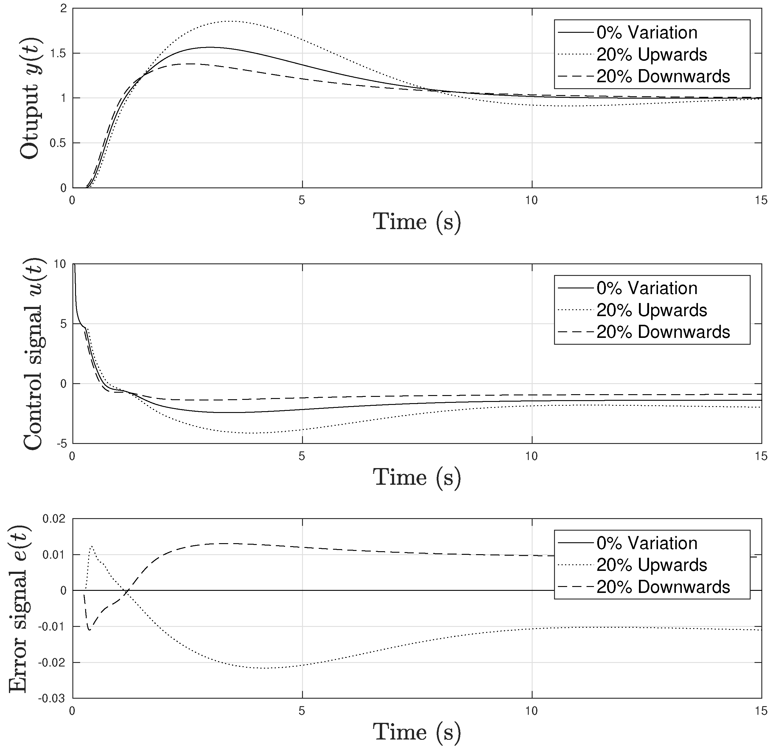
4.1. Example 1: Delayed System with One Unstable Pole

This example is a modification of the system presented in Ref. [25], where an unstable pole has been removed. It is a second order system with delay and one unstable pole represented by the transfer function,
G ( s ) = 17.8571 e 0.25 s ( s + 10 ) ( s + 5 ) ( s 0.5 ) .
From Theorem 3, τ < 4 is obtained, therefore for τ = 0.25 , there exists an observer with gains F = 0.392 1.96 , g 1 = 20 and a PID controller with k p = 10 , k i = 2 and k d = 3 , such that the closed-loop system is stable.
Figure 5 shows the time evolution of the output signal y ( t ) , the control signal u ( t ) and the signal error e ( t ) of the controlled system (39) for a unit step reference under three different conditions. First, the evolution of the system for the original parameters and how to analyze the robustness properties of the system under parametric uncertainties was considered, and then we considered the variation of the system’s parameters 20% up of the nominal values,
G ( s ) = 21.42852 e 0.3 s ( s + 12 ) ( s + 6 ) ( s 0.6 )
and 20% down producing,
G ( s ) = 14.28568 e 0.2 s ( s + 8 ) ( s + 4 ) ( s 0.4 ) .
From Figure 5, good performance of the system under the mentioned conditions is obvious.
As a second experiment, for system (39) a large time delay, i.e., τ = 2 , is considered. For this case, we obtained k p = 4.2 , k i = 0.2 and k d = 4.6 for the PID and F = 0.392 1.96 , g 1 = 20 . Figure 6, shows the time evolution of the signals y ( t ) , u ( t ) and e ( t ) where the adequate convergence is clearly stated.

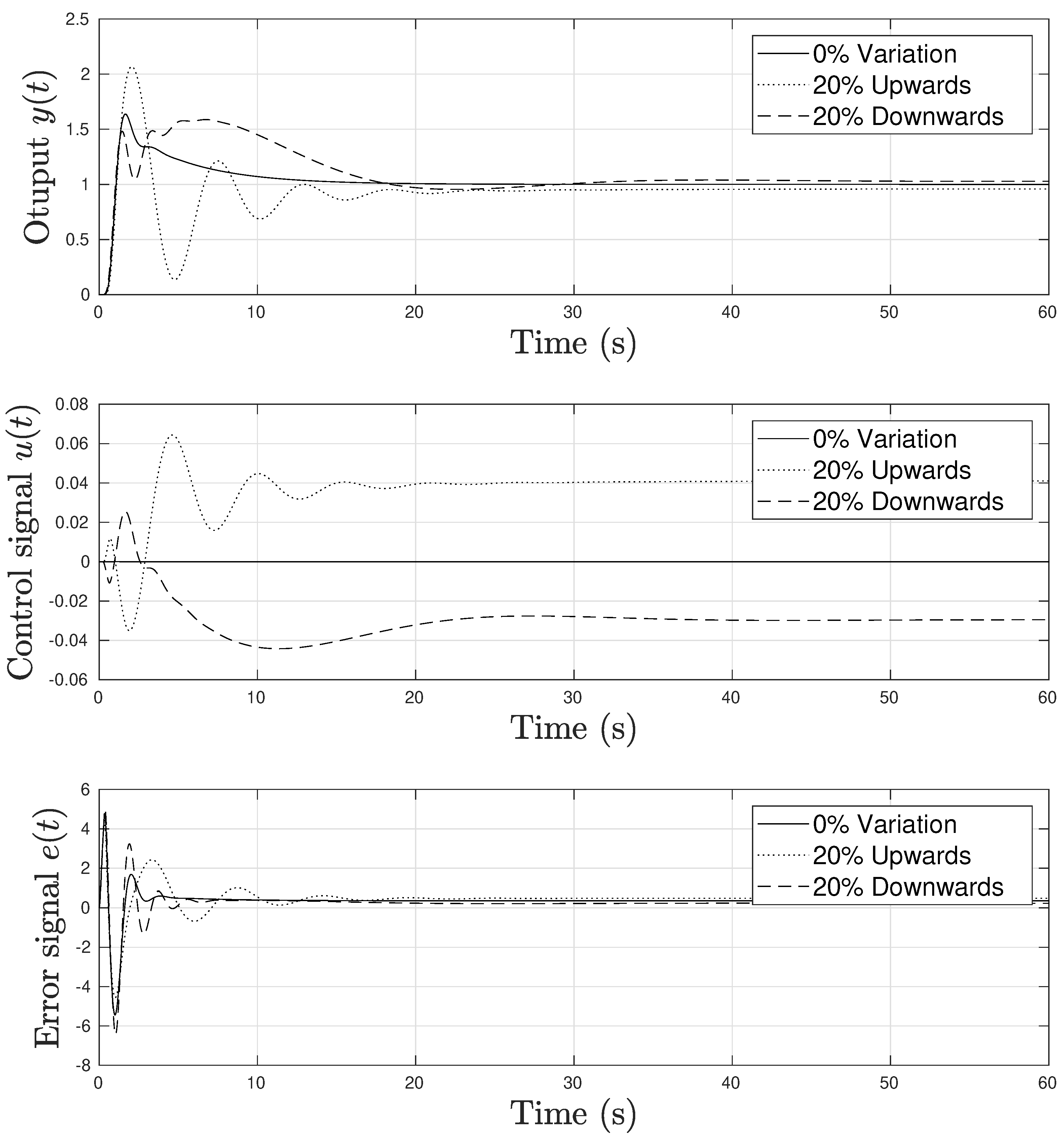
4.2. Example 2: Fourth Order Linear System with Delay and Two Unstable Poles

The two unstable poles case is evaluated by means of the following system, which was taken from Ref. [25],
G ( s ) = 17.8571 e 0.25 s ( s + 10 ) ( s + 5 ) ( s 0.7143 ) ( s 0.5 ) .
Following Ref. [25], it is possible stabilize the system (40) by means of a P D controller, if and only if, τ < 0.6485 . In addition, it is possible to observe that the conditions in Theorem 2 are fulfilled, obtaining the condition τ < 2 . Therefore, for τ = 0.25 there exists a PID controller with k p = 200 , k i = 30 and k d = 40 and feedback gains F = 1.216 16.5566 112.2496 , G = 20 20 so that the closed-loop system from Figure 3 is stable. Figure 7 shows the output signal y ( t ) , the control signal u ( t ) and the error signal e ( t ) and makes a comparison between the solution presented in this work and the P D proposed in Ref. [25] for k p = 0.7 and k d = 4.2 .
In addition, to analyze the robustness of the two unstable poles case, the parameters of the original system (40) are perturbed 20% up and 20% down resulting the transfer functions,
G ( s ) = 21.42852 e 0.3 s ( s + 12 ) ( s + 6 ) ( s 0.85716 ) ( s 0.6 )
and
G ( s ) = 14.28568 e 0.2 s ( s + 8 ) ( s + 4 ) ( s 0.57144 ) ( s 0.4 ) .
Figure 8 shows the time evolution of y ( t ) , u ( t ) and e ( t ) where the appropriate convergence of the error signal is evident.

4.3. Example 3: Three Unstable Poles

For the case of three unstable poles consider the system,
G ( s ) = e 0.5 s ( s + 0.1 ) ( s 0.1 ) ( s 0.2 ) ( s 0.3 ) .
From Theorem 1, τ < m i n ( 3.3333 , 3.8197 ) is obtained, producing the bound τ < 3.3333 . Therefore, for τ = 0.5 there exists an observer-based PID controller such that the closed-loop system is stable. The gains F = 10.1 1.1 10.3 , G = 26 10 , k p = 1 , k i = 0.1 and k d = 9.5 are considered. Figure 9, shows the dynamic response of the output y ( t ) , the control u ( t ) , and the error signal e ( t ) for a unit step reference considering the original system (41) and the corresponding transfer function obtained by parameters variation of 20% up and 20% down, given as,
G ( s ) = e 0.6 s ( s + 0.12 ) ( s 0.12 ) ( s 0.24 ) ( s 0.36 )
and
G ( s ) = e 0.4 s ( s + 0.08 ) ( s 0.08 ) ( s 0.16 ) ( s 0.24 )

5. Conclusions

In order to look for a general scheme that allows to stabilize unstable linear delayed systems of high order, we proposed in this work a general scheme that allows to deal with systems containing one, two, or three unstable poles. The proposed strategy is based on an observer (predictor) based PID controller that allows to achieve step tracking references. Necessary and sufficient conditions were stated depending on the parameters of the system and the delay size, to guarantee the existence of the stabilizing controller. Thanks to the proposed controller structure, the presented results are less restrictive than those reported in the literature dealing with one [16,17], or two unstable poles [25], when using a PID controller directly. Concerning delayed systems with three unstable poles, results reported in the literature concerning this situation do not exist, to the best of our best knowledge,. It is important to note that the proposed controller structure is the same for the three considered situations. Finally, the use of the results is illustrated by three academic examples, showing adequate performance.

Author Contributions

Conceptualization, C.C.-D. and B.d.M.-C.; methodology, C.C.-D. and B.d.M.-C.; formal analysis, M.V.-V. and J.F.M.-R.; validation, G.D.-S. All authors have read and agreed to the published version of the manuscript.

Funding

This research received no external funding.

Institutional Review Board Statement

Not applicable.

Informed Consent Statement

Not applicable.

Data Availability Statement

Not applicable.

Acknowledgments

The first author acknowledges support from CONACYT through a scholarship to pursue postgraduate studies at Instituto Politécnico Nacional.

Conflicts of Interest

The authors declare no conflict of interest.

References

  1. Chen, W.C. Dynamics and control of a financial system with time-delayed feedbacks. Chaos Solitons Fractals 2008, 37, 1198–1207. [Google Scholar] [CrossRef]
  2. Milton, J.G. Time delays and the control of biological systems: An overview. IFAC-PapersOnLine 2015, 48, 87–92. [Google Scholar] [CrossRef]
  3. Hamdy, M.; Ramadan, A. Design of Smith Predictor and Fuzzy Decoupling for Mimo Chemical Processes with Time Delays. Asian J. Control 2017, 19, 57–66. [Google Scholar] [CrossRef]
  4. Deng, M.; Inoue, A. Networked non-linear control for an aluminum plate thermal process with time-delays. Int. J. Syst. Sci. 2008, 39, 1075–1080. [Google Scholar] [CrossRef]
  5. Al-Wais, S.; Khoo, S.; Lee, T.H.; Shanmugam, L.; Nahavandi, S. Robust H cost guaranteed integral sliding mode control for the synchronization problem of nonlinear tele-operation system with variable time-delay. ISA Trans. 2018, 72, 25–36. [Google Scholar] [CrossRef]
  6. Min, H.; Wang, S.; Sun, F.E.A. Robust consensus for networked mechanical systems with coupling time delay. Int. J. Control Autom. Syst. 2012, 10, 227–237. [Google Scholar] [CrossRef]
  7. Zhang, C.K.; Jiang, L.; Wu, Q.H.; He, Y.; Wu, M. Delay-Dependent Robust Load Frequency Control for Time Delay Power Systems. IEEE Trans. Power Syst. 2013, 28, 2192–2201. [Google Scholar] [CrossRef]
  8. Bolognani, S.; Ceschia, M.; Mattavelli, P.; Paccagnella, A.; Zigliotto, M. Improved FPGA-based dead time compensation for SVM inverters. In Proceedings of the Second International Conference on Power Electronics, Machines and Drives (PEMD 2004), Edinburgh, UK, 31 March–2 April 2004; Volume 2, pp. 662–667. [Google Scholar]
  9. Deng, W.; Yao, J.; Wang, Y.; Yang, X.; Chen, J. Output feedback backstepping control of hydraulic actuators with valve dynamics compensation. Mech. Syst. Signal Process. 2021, 158, 107769. [Google Scholar] [CrossRef]
  10. Tang, Y.; Xing, X.; Karimi, H.R.; Kocarev, L.; Kurths, J. Tracking Control of Networked Multi-Agent Systems Under New Characterizations of Impulses and Its Applications in Robotic Systems. IEEE Trans. Ind. Electron. 2016, 63, 1299–1307. [Google Scholar] [CrossRef]
  11. Sipahi, R.; Niculescu, S.I.; Abdallah, C.T.; Michiels, W.; Gu, K. Stability and Stabilization of Systems with Time Delay. IEEE Control Syst. Mag. 2011, 31, 38–65. [Google Scholar]
  12. Smith, O.J.M. Closer Control of Loops With Dead Time. Chem. Eng. Prog. 1957, 53, 217–219. [Google Scholar]
  13. Rao, A.S.; Rao, V.S.R.; Chidambaram, M. Simple Analytical Design of Modified Smith Predictor with Improved Performance for Unstable First-Order Plus Time Delay (FOPTD) Processes. Ind. Eng. Chem. Res. 2007, 46, 4561–4571. [Google Scholar] [CrossRef]
  14. Levine, W.S. The Control Handbook—Electrical Engineering Handbook, 1st ed.; CRC-Press: Boca Raton, FL, USA, 1996; Volume 1. [Google Scholar]
  15. Wu, Z.; Yuan, J.; Li, D.; Xue, Y.; Chen, Y. The proportional-integral controller design based on a Smith-like predictor for a class of high order systems. Trans. Inst. Meas. Control 2021, 43, 875–890. [Google Scholar] [CrossRef]
  16. Lee, S.C.; Wang, Q.G.; Xiang, C. Stabilization of all-pole unstable delay processes by simple controllers. J. Process Control 2010, 20, 235–239. [Google Scholar] [CrossRef]
  17. Hernández-Pérez, M.A.; del Muro-Cuéllar, B.; Velasco-Villa, M. PID for the stabilization of high-order unstable delayed systems with possible complex conjugate poles. Asia-Pac. J. Chem. Eng. 2015, 10, 687–699. [Google Scholar] [CrossRef]
  18. Zhang, Z.; Wang, Q.G.; Zhang, Y. Relationship on Stabilizability of LTI Systems by P and PI Controllers. Can. J. Chem. Eng. 2007, 85, 374–377. [Google Scholar] [CrossRef]
  19. Novella Rodríguez, D.F.; del Muro-Cuéllar, B.; Sename, O. Observer-based scheme for the control of high order systems with two unstable poles plus time delay. Asia-Pac. J. Chem. Eng. 2014, 9, 167–180. [Google Scholar] [CrossRef] [Green Version]
  20. Vázquez, C.; Márquez, J.; del Muro, B.; Novella, D.; Hernandez, M.; Duchen, G. Observer-PI scheme for the stabilization and control of high order delayed systems with one or two unstable poles. IFAC-PapersOnLine 2018, 51, 432–437. [Google Scholar] [CrossRef]
  21. Rosas, C.D.V.; Rubio, J.F.M.; del Muro Cuéllar, B.; Rodríguez, D.F.N.; Sename, O.; Dugard, L. Stabilizing High-order Delayed Systems with Minimum-phase Zeros Using Simple Controllers. Stud. Inform. Control 2019, 28, 381–390. [Google Scholar]
  22. Duchén, G.; BDM, B.; Márquez, J.; Hernández, M.; Ramírez, E.; Cruz, C. Estabilización y control de sistemas de alto orden con retardo y dos polos inestables: Esquema PD-observador. In Proceedings of the Congreso Nacional de Control Automático, Puebla, Mexico, 23–25 October 2019; pp. 291–296. [Google Scholar]
  23. Duchén Sánchez, G.; del Muro Cuéllar, B.; Márquez Rubio, J.F.; Velasco Villa, M.; Hernández Pérez, M.A. Observer-Based PD Controller for a Class of High Order Linear Unstable Delayed Systems. IEEE Lat. Am. Trans. 2021, 100, 291–300. [Google Scholar] [CrossRef]
  24. Dev, A.; Novella Rodríguez, D.F.; Anand, S.; Sarkar, M.K. Multi Observer-Based Sliding Mode Load Frequency Control With Input Delay Estimation. ASME Lett. Dyn. Syst. Control 2021, 1, 041009. [Google Scholar] [CrossRef]
  25. Novella-Rodríguez, D.F.; del Muro Cuéllar, B.; Márquez-Rubio, J.F.; Hernández-Pérez, M.A.; Velasco-Villa, M. PD-PID controller for delayed systems with two unstable poles: A frequency domain approach. Int. J. Control 2019, 92, 1196–1208. [Google Scholar] [CrossRef]
Figure 1. PID controller strategy.
Mathematics 10 01399 g001
Figure 2. Proposed injection scheme. Three unstable poles case.
Mathematics 10 01399 g002
Figure 3. Observer-based PID control scheme.
Mathematics 10 01399 g003
Figure 4. System in state space.
Mathematics 10 01399 g004
Figure 5. Response for one unstable pole with parameters variations for τ = 0.25 .
Mathematics 10 01399 g005
Figure 6. Time evolution of the closed-loop system with one unstable pole for τ = 2 .
Mathematics 10 01399 g006
Figure 7. Comparison of methodologies for τ = 0.25 .
Mathematics 10 01399 g007
Figure 8. Response for two unstable poles with parameters variations.
Mathematics 10 01399 g008
Figure 9. Response for three unstable poles for τ = 0.5 .
Mathematics 10 01399 g009
Publisher’s Note: MDPI stays neutral with regard to jurisdictional claims in published maps and institutional affiliations.

