Boundary Controller Design for a Class of Horizontal Belt Transmission System with Boundary Vibration Constraint

Abstract

In this paper, the problem of transverse vibration suppression of a belt system moving in the horizontal direction is investigated. This system is characterized by the boundary vibration constraint and is affected by external disturbances. For it, we introduced a logarithmic function in the candidate term of the Lyapunov function and used a symbolic function in the controller to compensate for the effects of boundary vibration constraints and boundary disturbances, respectively. In order to better achieve the control objective, we designed a boundary control scheme. The state feedback boundary controller was designed using the boundary signals of the system when they can be available directly. Considering the presence of noise in the practical system, some system signals cannot be measured accurately. Therefore, a high-gain observer was introduced to estimate these signals, and an output feedback boundary controller was designed. Finally, the simulation example showed that both controllers guarantee effective suppression of the transverse vibration of the system without violating the boundary vibration constraints.

1. Introduction

Compared with the traditional rigid structure, the flexible structure has the characteristics of low cost, high flexibility, and high energy efficiency. Therefore, flexible systems are widely used [1,2,3,4]. In practical engineering, harmful transverse vibrations can be generated due to the influence of external disturbances and the physical structure characteristics of the system itself, which may reduce the productivity of the system. To solve those unwanted vibrations, the first step is to establish an accurate flexible system model. The dynamic model of flexible system is essentially a distributed parameter system with infinite dimensional state space. If we use the traditional finite-dimensional approximation method, it has some advantages in system structure analysis and controller design, but it will cause the loss of system signal and seriously affect the performance of the controller. Using partial differential equations (PDEs) to model distributed parameter systems can avoid such disadvantages. Therefore, we use partial differential equations to build the system model. This modeling approach has been widely used in practical systems, such as submarine resource transmission operation [5], wind power plant [6], and satellite attitude adjustment [7], and so on.

Up to now, the boundary control problem has become the most common problem in flexible systems modeled by PDEs [8,9,10,11]. In the boundary control scheme, sensors and actuators are placed at the boundary of the system, which not only does not affect the modeling and analysis of other locations of the flexible system, but is also easy to implement [12,13]. In fact, there have been many research results in the field of boundary control [14,15,16,17,18,19,20,21,22,23,24]. Boundary controllers have been used to suppress vibrations of systems modeled as flexible strings [14,15]. The Lyapunov direct method was used to design boundary control schemes to achieve the reduction in additional vibrations of the system [16,17]. In [18,19,20,21,22], a boundary feedback strategy was proposed to achieve the control of the angle and the reduction in the system’s vibration objective by designing the controller and the observer simultaneously. In [23], the solution of the closed-loop system is constructed and the existence of the solution is proved by constructing a suitable Lyapunov function and proving the exponential stability of the system, using the Galerkin approximation scheme. It is worth noting that the two ends of the above physical system are the free end and the fixed end, respectively. However, for an axially moving flexible system with fixed ends, we cannot simply use the control scheme mentioned in the above references if we want to achieve better control results.

A belt, as a typical axially moving flexible structural system, whose transverse vibration always produces huge noise, will pollute the environment. In order to improve the transmission and control efficiency of the belt system, scholars have put forward many useful control strategies. In [24], a boundary control scheme for an auxiliary system was proposed to deal with the problem using actuator saturation constraint. In [25], by a combination of adaptive technology and the Lyapunov analysis method, authors put forward adaptive boundary control to suppress belt transverse vibration and design adaptive law for the influence of unknown system parameters to deal with the situation that some variables of the belt system are unknown. In [26], the adaptive method is used to deal with the uncertainty of parameters and interfere with observers to eliminate the influence of unknown boundary disturbances. In [27], the boundary controller is designed by the Lyapunov function to suppress vibration, while the axially moving belt system is divided into a controllable domain and an uncontrollable domain. In the references mentioned above, we find that there is little information about the boundary vibration constraint of an axially moving belt system. For the belt system, the boundary vibration constraint problem is worth paying attention to and solving. In general, the speed of the belt operation varies according to the different production requirements. Due to the limited tension of the belt system material and the physical characteristics of the close connection between the rotating shaft and the belt, the transverse vibration of the belt must not exceed the safe range. Once the transverse vibration exceeds the system boundary vibration constraint, coupled with the belt variable speed motion, it will reduce the efficiency of the belt and damage the belt system in severe cases. Taking the system boundary vibration constraint into account in the control scheme design will make the controller design more challenging.

In addition, in the above references, the authors assume that the state information of the system can be obtained by sensors or corresponding algorithms, and designed a state control scheme based on these signals. However, due to the existence of noise in the actual system, the measurement of some system signals will be inaccurate. To avoid this problem, we introduce a high-gain observer to estimate these system signals. The introduction of the observer increases the challenge of the controller design scheme [28,29,30].

In this paper, we consider the variable speed horizontal belt conveying system of surface mount technology equipment (SMTs) with boundary displacement restrain as model analysis. A form of the Lyapunov function, combining both the logarithmic function and the integral Lyapunov function, is employed for the control design and stability analysis of the axially moving belt system. According to the availability of the second derivative of the system signal, a state feedback controller and an output feedback controller are designed, respectively, and a high-gain observer is used in the design of the output feedback control scheme.

Compared with the existing results of belt systems, the main contributions of this paper can be summarized by the following two points:

(1)

The problem of the boundary vibration constraints is considered. To the best of our knowledge, there are few research results on the boundary vibration constraint problem of belt systems. However, as far as the controllable area of the whole belt system is concerned, the vibration at the boundary is more intense. If the vibration at the boundary can satisfy the physical constraint of the belt system, then the whole belt system will not produce a strong transverse vibration.

(2)

In practice, since the influence of many factors can make the measurement of the system boundary signal inaccurate, the control effect will be inevitably affected if the state feedback control scheme is used. For this reason, we designed a high-gain observer to observe the boundary signals and designed an output feedback control scheme based on the observed signals.

The remaining structure of this paper is as follows. In Section 2, the dynamic equations of the system and the controller objectives we need to achieve are given. In Section 3, the design method of the state and output feedback controller and the stability analysis of the closed-loop system are given. In Section 4, the simulation results show the effectiveness of the designed controller, and the conclusion is provided in Section 5.

2. System Description and Control Objectives

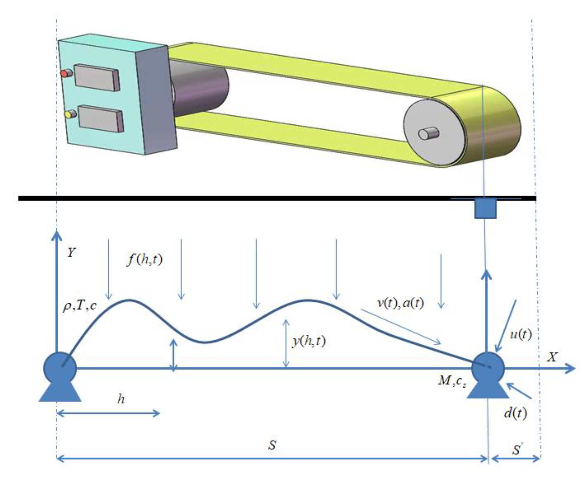
As shown in Figure 1, this paper studies a class of horizontal belt transmission systems with the boundary vibration constraint. The parameters of the system and the meanings of the relevant variables are described in detail in

Table 1. Parameter description of the system.

Parameter	Description
$y\left(h,t\right)$	the vibration offset of the belt system that varies with time t and space h
$S$	the distance between the actuator and the steering roller
$\rho$	the density of the belt system materials
$M$	the total carrier mass of the actuator at the right boundary of the controllable domain
$c$	the viscous damping coefficient of the belt
$c_s$	the damping coefficient produced by the actuator during operation
$T$	the belt tension that does not change with time and space
$v\left(t\right)$	the variable horizontal conveying speed of the belt system
$a\left(t\right)$	the speed change per unit time
$u$	the control input
$S^{\prime }$	the distance between the actuator and its right power roller
$d\left(t\right)$	the boundary disturbance
$f\left(h,t\right)$	the unknown and bounded distributed disturbance

. The following abbreviations are defined for later interpretation:

$$\left(\cdot \right)\left(h,t\right)=\left(\cdot \right),{\left(\cdot \right)}_h=\frac{\partial \left(\cdot \right)}{\partial h},{\left(\cdot \right)}_t=\frac{\partial \left(\cdot \right)}{\partial t},{\left(\cdot \right)}_{hh}=\frac{{\partial }^2\left(\cdot \right)}{\partial h^2},{\left(\cdot \right)}_{tt}=\frac{{\partial }^2\left(\cdot \right)}{\partial t^2},{\left(\cdot \right)}_{ht}=\frac{\partial \left(\partial \left(\cdot \right)\right)}{\partial h\partial t}.$$

The belt system with horizontal transmission and controllable acceleration has a governing equation, which is given as [25]:

$$\rho y_{tt}+\left(\rho a+cv\right)y_h+2\rho v{y}_{ht}+\left(\rho v^2-T\right)y_{hh}+c{y}_t-f=0$$

(1)

for $\forall \left(h,t\right)\in \left(0,S\right)\times \left[\left.0,+\infty \right)\right.$. The dynamics at the boundary are given by the following equations:

$$\left\{\begin{array}{l}y\left(0,t\right)=0\\ M{y}_{tt}\left(S,t\right)+T{y}_h\left(S,t\right)+c_s{y}_t\left(S,t\right)-u-d=0\end{array}\right.$$

(2)

The control objectives of this paper are to design the boundary controller under the state feedback and the output feedback, respectively, which can reach the following aims: (1) suppress the transverse vibration $y\left(h,t\right)$ of the belt system and make it as small as possible; (2) keep the boundary vibration so that it will not exceed the boundary of restraint, i.e., to assure $y\left(S,t\right)$ achieves $\left|y\left(S,t\right)\right|<l_0$, where $l_0$ is a constant value that the boundary vibration cannot exceed due to the limitation of the belt system.

3. Boundary Control Design

In this paper, we take two system conditions into consideration: (i) the state feedback boundary control and (ii) the output feedback boundary control. In case (i), all system signals are directly obtained by sensors and the backward difference algorithms. As for case (ii), $y_{ht}(S,t)$ is unmeasurable and is estimated by the high-gain observer.

For the follow-up analysis, the following lemmas and assumptions are introduced first.

Lemma 1

([25]). Let $n_1\left(h,t\right)$, $n_2\left(h,t\right)\in R$, $P>0$ with $\left[0,S\right]\times \left[\left.0,\infty \right)\right.$, then there are the following two inequalities hold

$$\left\{\begin{array}{l}{n}_1{n}_2\le \left|n_1{n}_2\right|\le \frac{n_1^2}{2}+\frac{n_2^2}{2}\le n_1^2+n_2^2\\ \left|n_1{n}_2\right|=\left|\left(\frac{1}{\sqrt{P}}{n}_1\right)\left(\sqrt{P}{n}_2\right)\right|\le \frac{1}{P}{n}_1^2+P{n}_2^2\end{array}\right.$$

(3)

Lemma 2

([31]). Let $n\left(h,t\right)\in R\left(\left(h,t\right)\in \left[0,S\right]\times \left[\left.0,\infty \right)\right.\right)$ be a function with the domain of two independent variables, which satisfies the initial position is zero at any time, then there will be an inequality of the following form

$$n^2\le S{\displaystyle {\int }_0^S{n}_h^{2}dh}$$

(4)

Lemma 3

([32]). When the kinetic energy and potential energy of system are bounded $\forall t\in [0,+\infty )$, the states $y_h(h,t)$, $y_t(h,t)$, $y_{hh}(h,t)$, and $y_{ht}(h,t)$ are deduced to be bounded $\forall h\in [0,S]$, $t\in \left[0,+\infty \right)$.

Assumption 1.

Assume that$v\left(t\right)$,$a\left(t\right)$,$d\left(t\right)$, and$f\left(h,t\right)$mentioned in (1) and (2) are bounded. That is to say, there are some constants$q_1$,$q_2$,$\overline{d}$, and$q_3$, such that$0\le v\left(t\right)\le q_1$,$\left|a\left(t\right)\right|\le q_2$,$\left|d\left(t\right)\right|\le \overline{d}$, and$\left|f\left(h,t\right)\right|\le q_3$, for$\forall t\in \left[0,\infty \right)$.

This is an appropriate assumption. Because the power provided by the power roller cannot be large, wirelessly, $v\left(t\right)$, $a\left(t\right)$, and $f\left(h,t\right)$ are generated by their boundaries. The boundary interference $d\left(t\right)$ has limited energy, so it is also bounded.

3.1. State Feedback Boundary Controller Design

In this part, to keep the boundary displacement remaining in the constrained space, in the case where all the parameters in the considered system are known, the state feedback boundary control scheme is proposed. The Lyapunov stability theory will be applied to prove the system’s stability, and the design process of the controller is described as follows.

The following Lyapunov function is chosen

$$V\left(t\right)=V_a\left(t\right)+V_b\left(t\right)+V_c\left(t\right)$$

(5)

where

$$V_a\left(t\right)=\frac{1}{2}\gamma \rho {\displaystyle {\int }_0^S{\left(y_t+v{y}_h\right)}^{2}dh}+\frac{1}{2}\gamma T{\displaystyle {\int }_0^S{y}_h^{2}dh}$$

(6)

$$V_b\left(t\right)=2\lambda \rho {\displaystyle {\int }_0^{S}h{y}_h\left(y_t+v{y}_h\right)dh}$$

(7)

$$V_c\left(t\right)=\frac{1}{2}M{z}_2^2\ln \frac{2l_0^2}{l_0^2-z_1^2}$$

(8)

with $\gamma >0$ and $\lambda >0$ being design parameters, $l_0$ being the boundary vibration constrained bound. $z_1$ and $z_2$ are the auxiliary signals, which are defined as

$$\left\{\begin{array}{l}{z}_1=y\left(S,t\right)\\ z_2=y_t\left(S,t\right)+k_1{y}_h\left(S,t\right)\end{array}\right.$$

(9)

where $k_1>0$ is constant.

Applying Lemma 1 to $V_b\left(t\right)$ yields

$$\left|V_b\left(t\right)\right|\le \lambda \rho S{\displaystyle {\int }_0^S\left[y_h^2+{\left(y_t+v{y}_h\right)}^2\right]dh}\le \mu V_a\left(t\right)$$

(10)

where

$$\mu =\frac{2\lambda \rho S}{\min \left(\gamma \rho ,\gamma T\right)}$$

(11)

Then, we can obtain the following results by appropriately selecting the values of $\gamma$ and $\lambda$

$$\left\{\begin{array}{l}{\mu }_1=1-\frac{2\lambda \rho S}{\min \left(\gamma \rho ,\gamma T\right)}=1-\mu >0\\ {\mu }_2=1+\frac{2\lambda \rho S}{\min \left(\gamma \rho ,\gamma T\right)}=1+\mu >1\end{array}\right.$$

(12)

Further, it holds that

$$0<{\mu }_1{V}_a\left(t\right)\le V_a\left(t\right)+V_b\left(t\right)\le {\mu }_2{V}_a\left(t\right)$$

(13)

Then, from (5), we have

$$0<{\mu }_1\left[V_a\left(t\right)+V_c\left(t\right)\right]\le V\left(t\right)\le {\mu }_2\left[V_a\left(t\right)+V_c\left(t\right)\right]$$

(14)

Therefore, we find that $V(t)$ is bounded and greater than zero.

Using (5), and taking the derivative of $V(t)$ along with time, we have

$$V_t\left(t\right)=V_{at}\left(t\right)+V_{bt}\left(t\right)+V_{ct}\left(t\right)$$

(15)

Substituting (1) into $V_{at}\left(t\right)$, we have

$$\begin{array}{ll}{V}_{at}\left(t\right)& =\gamma \rho {\displaystyle {\int }_0^S\left(y_t+v{y}_h\right)\left(y_{tt}+v{y}_{ht}+a{y}_h\right)dh}+\gamma T{\displaystyle {\int }_0^S{y}_h{y}_{ht}dh}\\ & =\frac{\gamma Tv}{2}{y}_h^2\left(S,t\right)-\frac{\gamma v\left(T-\rho v^2\right)}{2}{y}_h^2\left(0,t\right)\\ & \hspace{1em}-\frac{\gamma \rho v}{2}{\left(y_t\left(S,t\right)+v{y}_h\left(S,t\right)\right)}^2+\frac{\gamma T}{2k_1}{z}_2^2\\ & \hspace{1em}-\frac{\gamma T}{2k_1}{y}_t^2\left(S,t\right)-\frac{\gamma T{k}_1}{2}{y}_h^2\left(S,t\right)\\ & \hspace{1em}+\gamma {\displaystyle {\int }_0^S\left(y_t+v{y}_h\right)\left(f-c\left(y_t+v{y}_h\right)\right)dh}\end{array}$$

(16)

Similarly, based on (1), we can obtain $V_{bt}(t)$ as

$$\begin{array}{ll}{V}_{bt}\left(t\right)& =2\lambda \rho {\displaystyle {\int }_0^{S}h{y}_{ht}\left(y_t+v{y}_h\right)+h{y}_h\left(y_{tt}+v{y}_{ht}+a{y}_h\right)dh}\\ & =\lambda \rho S{y}_t^2\left(S,t\right)-\left(\lambda \rho S{v}^2-\lambda ST\right)y_h^2\left(S,t\right)-\lambda \rho {\displaystyle {\int }_0^S{y}_t^{2}dh}+\lambda \left(\rho v^2-T\right){\displaystyle {\int }_0^S{y}_h^{2}dh}\\ & +2\lambda {\displaystyle {\int }_0^{S}h{y}_h\left(f-c\left(y_t+v{y}_h\right)\right)dh}\end{array}$$

(17)

Using the boundary condition (2), we can see that

$$V_{ct}\left(t\right)=\frac{z_1{y}_t\left(S,t\right)}{l_0^2-z_1^2}M{z}_2^2+z_2\ln \frac{2l_0^2}{l_0^2-z_1^2}(u+d-T{y}_h(S,t)-c_s{y}_t(S,t)+M{k}_1{y}_{ht}(S,t))$$

(18)

In order to achieve control objectives, the state feedback controller is designed as

$$\begin{array}{ll}u=& \frac{-k_2{z}_2}{\ln \frac{2l_0^2}{l_0^2-z_1^2}}-\frac{M{z}_1{y}_t(S,t)z_2}{(l_0^2-z_1^2)\ln \frac{2l_0^2}{l_0^2-z_1^2}}-k_3{z}_2+T{y}_h\left(S,t\right)+c_s{y}_t\left(S,t\right)\\ & -M{k}_1{y}_{ht}\left(S,t\right)-sign\left(z_2\right)\overline{d}\end{array}$$

(19)

where $k_2>0$ and $k_3>0$ are constants.

Combining with (19) and (18), we can obtain

$$\begin{array}{ll}{V}_{ct}\left(t\right)& =\frac{z_1{y}_t\left(S,t\right)}{l_0^2-z_1^2}M{z}_2^2+z_2\ln \frac{2l_0^2}{l_0^2-z_1^2}(u+d-T{y}_h(S,t)-c_s{y}_t(S,t)+M{k}_1{y}_{ht}(S,t))\\ & \le -k_2{z}_2^2-k_3{z}_2^2\ln \frac{2l_0^2}{l_0^2-z_1^2}+z_2\ln \frac{2l_0^2}{l_0^2-z_1^2}\left(d-\mathrm{sign}\left(z_2\right)\overline{d}\right)\\ & \le -k_2{z}_2^2-k_3{z}_2^2\ln \frac{2l_0^2}{l_0^2-z_1^2}\end{array}$$

(20)

From (15)–(17) and (20), we have

$$\begin{array}{ll}{V}_t\left(t\right)\le & -\left(\frac{\gamma T}{2k_1}-\lambda \rho S\right)y_t^2\left(S,t\right)-\frac{\gamma v\left(T-\rho v^2\right)}{2}{y}_h^2\left(0,t\right)\\ & -k_3{z}_2^2\ln \frac{2l_0^2}{l_0^2-z_1^2}-\frac{\gamma \rho v}{2}{\left(y_t\left(S,t\right)+v{y}_h\left(S,t\right)\right)}^2\\ & -\left(k_2-\frac{\gamma T}{2k_1}\right)z_2^2-\left(\lambda \rho S{v}^2+\frac{\gamma T\left(k_1-v\right)}{2}-\lambda ST\right)y_h^2\left(S,t\right)\\ & -\left(c\gamma -\gamma k_4-\frac{2\lambda cS}{k_6}\right)\times {\displaystyle {\int }_0^S{\left(y_t+v{y}_h\right)}^{2}dh}+\left(\frac{\gamma }{k_4}+\frac{2\lambda S}{k_5}\right){\displaystyle {\int }_0^S{f}^{2}dh}\\ & -\left(\lambda T-\lambda \rho q_1{}^2-2\lambda S{k}_5-2\lambda cS{k}_6\right){\displaystyle {\int }_0^S{y}_h^{2}dh}\end{array}$$

(21)

where $k_4>0$, $k_5>0$ and $k_6>0$ are constants.

Appropriate parameters are chosen to make the following inequality hold

$$\left\{\begin{array}{l}\lambda <\frac{\min \left(\gamma T,\gamma \rho \right)}{2\rho S},\frac{\gamma v(T-\rho v^2)}{2}\ge 0\\ {\pi }_1=c\gamma -\gamma k_4-\frac{2\lambda cS}{k_6}>0\\ {\pi }_2=\lambda T-\lambda \rho q_1^2-2\lambda S{k}_5-2\lambda cS{k}_6>0\\ \frac{\gamma T}{2k_1}-\lambda \rho S\ge 0,k_2-\frac{\gamma T}{2k_1}>0\\ \lambda \rho S{v}^2+\frac{\gamma T\left(k_1-v\right)}{2}-\lambda ST\ge 0\end{array}\right.$$

(22)

then, we deduce that

$$\begin{array}{ll}{V}_t\left(t\right)& \le -{\pi }_1{\displaystyle {\int }_0^S{\left(y_t+v{y}_h\right)}^{2}dh}-{\pi }_2{\displaystyle {\int }_0^S{y}_h^2}dh\\ & -k_3{z}_2^2\ln \frac{2l_0^2}{l_0^2-z_1^2}+\varpi \\ & \le -{\mu }_3\left[V_a\left(t\right)+V_c\left(t\right)\right]+\varpi \end{array}$$

(23)

where ${\mu }_3=\min \left(\frac{2{\pi }_1}{\gamma \rho },\frac{2{\pi }_2}{\gamma T},\frac{2k_3}{M}\right),0<\varpi =\left(\frac{\gamma }{k_4}+\frac{2\lambda S}{k_5}\right)S{q}_3^2<+\infty$.

Combining with (14) and (23), we further obtain

$$V_t\left(t\right)\le -\eta V\left(t\right)+\varpi$$

(24)

where $\eta =\frac{{\mu }_3}{{\mu }_2}$.

Theorem 1.

For a class of belt systems with horizontal transmission and variable speed represented by (1) and (2), under Assumption 1, if the initial state of the system is bounded and the inequality shown in (22) is satisfied by selecting appropriate parameters, then the designed controller (19) can guarantee that: (1) The vibration displacement of the system is stable near the equilibrium position; (2) All signals of the closed-loop system are bounded; and (3) The boundary vibration generated during the whole system operation will not exceed its constraint condition.

Proof of Theorem 1.

The boundedness of $y\left(h,t\right)$ is shown in the following.

After integrating (24), we can obtain

$$V\left(t\right)\le V\left(0\right)e^{-\chi t}+\frac{\varpi }{\chi }$$

(25)

Then, for the boundedness of the initial state, we can see that $V\left(t\right)$ is bounded in any future time. Combining (4), (6) and (14), we have

$$\frac{\gamma T}{2S}{y}^2\left(h,t\right)\le \frac{\gamma T}{2}{\displaystyle {\int }_0^S{y}_h^{2}dh}\le V_a\left(t\right)\le V_a\left(t\right)+V_c\left(t\right)\le \frac{1}{{\mu }_1}V\left(t\right)$$

(26)

According to (26) and (25), we can conclude that

$$\left|y\left(h,t\right)\right|\le \sqrt{\frac{2S}{\gamma {\mu }_{1}T}\left[V\left(0\right)e^{-\chi t}+\frac{\varpi }{\chi }\right]}$$

(27)

for $\forall \left(h,t\right)\in \left[0,S\right]\times \left[\left.0,\infty \right)\right.$.

Furthermore, for $\forall h\in \left[0,S\right]$, a direct computation yields

$$\underset{t\to \infty }{\lim }\left|y\left(h,t\right)\right|\le \underset{t\to \infty }{\lim }\sqrt{\frac{2S}{\gamma {\mu }_{1}T}\left[V\left(0\right)e^{-\chi t}+\frac{\varpi }{\chi }\right]}=\sqrt{\frac{2S\varpi }{\gamma {\mu }_1\chi T}}$$

(28)

Based on (26), we find that $V_a(t)$ and $V_c(t)$ are bounded. According to the definition of $V_a(t)$, the states of the system $y_h(h,t)$ and $y_t(h,t)$ are also bounded $\forall \left(h,t\right)\in \left[0,S\right]\times \left[\left.0,+\infty \right)\right.$. Subsequently, the boundedness of the kinetic energy and the potential energy are ensured [25]. According to Lemma 3, we conclude that the signals $y_{hh}(h,t)$ and $y_{ht}(h,t)$ are bounded. According to (1), the state $y_{tt}(h,t)$ is also bounded. Hence, all signals of the closed-loop system are bounded.

Next, it is an indication that $y\left(S,t\right)$ satisfies its constrained condition, i.e., $-l_0<y\left(S,t\right)<l_0$,$\forall t\in \left[\left.0,\infty \right)\right.$.

It is assumed that the vibration at the right boundary of the system has $-l_0<y\left(S,0\right)<l_0$. Because of the definition of $V_c(t)$, we can obtain $V_c\left(t\right)\to \infty$, as $\left|y\left(S,t\right)\right|\to l_0$. However, the function of $V(t)$ is bounded, which contradicts with $V_c\left(t\right)\to \infty$. So given that $-l_0<y\left(S,0\right)<l_0$, we have $-l_0<y\left(S,t\right)<l_0$, $\forall t\in \left[0,\infty \right)$.

Because of the similarity of systems, interested readers can refer to [24] about the properties of system solutions. So, it is omitted here.

This completes the proof of Theorem 1. □

3.2. Output Feedback Boundary Controller Design

Different from the previous part, this section will explore the design of the boundary controller and the analysis of system stability when the second derivative of the system boundary signal cannot be directly used by the control scheme. The first derivative of the boundary signal of the system can be measured by sensors, so $y_t(S,t)$ and $y_h(S,t)$ can be used. For the existence of noise in actual systems, $y_{ht}(S,t)$ is unmeasured, which will affect the control performance. Therefore, a high-gain observer is used to estimate $y_{ht}(S,t)$, and a controller is designed by using the observed value.

Before designing, the following important lemma is given.

Lemma 4

([33]). Suppose that a system output $s\left(t\right)$ and its first $k$-order derivatives are bounded as $\left|s^{\left(k\right)}\right|<{\mathrm{\Xi }}_k$ with positive constants ${\mathrm{\Xi }}_k$, $k=1,\cdots ,n$, for the system

$$\left\{\begin{array}{l}\tau {\delta }_{it}={\delta }_{i+1},i=1,\cdots ,n-1\\ \tau {\delta }_{nt}=-{\overline{\lambda }}_1{\delta }_n-{\overline{\lambda }}_2{\delta }_{n-1}-\cdots -{\overline{\lambda }}_{n-1}{\delta }_2-{\delta }_1+x_1\end{array}\right.$$

(29)

where $\tau$ is a small positive constant, and the parameters ${\overline{\lambda }}_i$, for $i=1,\cdots ,n-1$, are chosen such that the polynomial $w^s+{\overline{\lambda }}_1{w}^{n-1}+\cdots +{\overline{\lambda }}_{n-1}w+1$ is Hurwitz. Then, we conclude the following property

$$x_k=\frac{{\delta }_k}{{\tau }^{k-1}}-x_1{}^{\left(k-1\right)}=-\tau {\zeta }^{\left(k\right)},k=1,\cdots ,n-1$$

(30)

where $\zeta ={\delta }_n+{\overline{\lambda }}_1{\delta }_{n-1}+\cdots +{\overline{\lambda }}_{n-1}{\delta }_1$ with ${\zeta }^{\left(k\right)}$ denoting the $k$-order derivative of $\zeta$. In addition, there exist positive constants $T^{\ast }$ and $h_k$ such that $\left|x_k\right|\le \tau h_k$, $k=1,\cdots ,n$, for $\forall t>T^{\ast }$.

It is obvious from Lemma 4 that $\frac{{\delta }_{k+1}\left(t\right)}{{\tau }^k}$ converges to $x_1{}^{\left(k\right)}\left(t\right)$, in which $x_1{}^{\left(k\right)}\left(t\right)$ represents the $k$-order derivative of $x_1\left(t\right)$. When $x_1\left(t\right)$ satisfies the above lemma, $x_1{}^{\left(k\right)}\left(t\right)$ will tend to zero due to the existence of high gain $\frac{1}{\tau }$. So, $\frac{{\delta }_{k+1}\left(t\right)}{{\tau }^k}$ is chosen as an observer to estimate the $k$-order derivative of the unmeasurable signal. In this paper, we define $x_1\left(t\right)=y_h\left(S,t\right)$, $x_2\left(t\right)=y_{ht}\left(S,t\right)$ and the estimated value of $x_2\left(t\right)$ is

$${\widehat{x}}_2=\frac{{\delta }_2}{\tau }$$

(31)

where

$$\left\{\begin{array}{l}\tau {\delta }_{1t}={\delta }_2\\ \tau {\delta }_{2t}=-{\overline{\lambda }}_1{\delta }_2-{\delta }_1+x_1\\ {\tilde{x}}_2={\widehat{x}}_2-x_2\end{array}\right.$$

(32)

The following Lyapunov function is chosen

$$V_0\left(t\right)=V_1\left(t\right)+V_2\left(t\right)+V_3\left(t\right)$$

(33)

where

$$V_1\left(t\right)=\frac{1}{2}\omega \rho {\displaystyle {\int }_0^S{\left(y_t+v{y}_h\right)}^{2}dh}+\frac{1}{2}\omega T{\displaystyle {\int }_0^S{y}_h^{2}dh}$$

(34)

$$V_2\left(t\right)=2\iota \rho {\displaystyle {\int }_0^{S}h{y}_h\left(y_t+v{y}_h\right)dh}$$

(35)

$$V_3\left(t\right)=\frac{1}{2}M{z}_3^2\ln \frac{2l_0^2}{l_0^2-z_1^2}$$

(36)

with $\omega >0$ and $\iota >0$ being design parameters. $z_1$ and $z_3$ are the auxiliary signals, which are defined as

$$\left\{\begin{array}{l}{z}_1=y\left(S,t\right)\\ z_3=y_t\left(S,t\right)+k_{10}{x}_1\end{array}\right.$$

(37)

where $k_{10}>0$ is constant.

Applying the same method as, selecting the appropriate parameters $\omega$ and $\iota$, it is easy to verify that

$$0<{\mu }_{10}{V}_1\left(t\right)\le V_1\left(t\right)+V_2\left(t\right)\le {\mu }_{20}{V}_1\left(t\right)$$

(38)

Then, from (33), we have

$$0<{\mu }_{10}\left[V_1\left(t\right)+V_3\left(t\right)\right]\le V_0\left(t\right)\le {\mu }_{20}\left[V_1\left(t\right)+V_3\left(t\right)\right]$$

(39)

where ${\mu }_{10}>0$ and ${\mu }_{20}>0$ are constants. Therefore, we find that $V_0(t)$ is bounded and greater than zero.

Using (33) and taking the derivative of $V_0(t)$ along with time, we find

$$V_{0t}\left(t\right)=V_{1t}\left(t\right)+V_{2t}\left(t\right)+V_{3t}\left(t\right)$$

(40)

Using the governing Equation (1), it yields

$$\begin{array}{c}{V}_{1t}\left(t\right)=\omega {\displaystyle {\int }_0^S\left(y_t+v{y}_h\right)\left(f-c\left(y_t+v{y}_h\right)\right)dh}+\frac{\omega Tv}{2}{x}_1^2-\frac{\omega v\left(T-\rho v^2\right)}{2}{y}_h^2\left(0,t\right)\\ -\frac{\omega \rho v}{2}{\left(y_t\left(S,t\right)+v{x}_1\right)}^2+\frac{\omega T}{2k_{10}}{z}_3^2-\frac{\omega T}{2k_{10}}{y}_t^2\left(S,t\right)-\frac{\omega T{k}_{10}}{2}{x}_1^2\end{array}$$

(41)

Similarly, based on (1) and substituting (1) into $V_{2t}\left(t\right)$, we have

$$\begin{array}{ll}{V}_{2t}\left(t\right)& =2\iota \rho {\displaystyle {\int }_0^S\left[h{y}_{ht}\left(y_t+v{y}_h\right)+h{y}_h\left(y_{tt}+v{y}_{ht}+a{y}_h\right)\right]dh}\\ & =\iota \rho S{y}_t^2\left(S,t\right)-\left(\iota \rho S{v}^2-\iota ST\right)x_1^2-\iota \rho {\displaystyle {\int }_0^S{y}_t^{2}dh}\\ & \hspace{1em}+2\iota {\displaystyle {\int }_0^{S}h{y}_h\left(f-c\left(y_t+v{y}_h\right)\right)dh}+\iota \left(\rho v^2-T\right){\displaystyle {\int }_0^S{y}_h^{2}dh}\end{array}$$

(42)

Using the boundary condition (2), we conclude that

$$\begin{array}{ll}{V}_{3t}\left(t\right)& =\frac{M{z}_1{y}_t\left(S,t\right)z_3^2}{l_0^2-z_1^2}+z_3\ln \frac{2l_0^2}{l_0^2-z_1^2}\left(M{y}_{tt}+M{k}_{10}{x}_2\right)\\ & =\frac{M{z}_1{y}_t\left(S,t\right)z_3^2}{l_0^2-z_1^2}+z_3\ln \frac{2l_0^2}{l_0^2-z_1^2}(u_0-T{y}_h(S,t)-c_s{y}_t(S,t)+d+m_c{k}_{10}{x}_2)\end{array}$$

(43)

In order to achieve control objectives, the output feedback controller is designed as

$$\begin{array}{ll}{u}_0=& \frac{-k_{20}{z}_3}{\ln \frac{2l_0^2}{l_0^2-z_1^2}}-\frac{M{z}_1{y}_t(S,t)z_3}{(l_0^2-z_1^2)\ln \frac{2l_0^2}{l_0^2-z_1^2}}-sign\left(z_3\right)\overline{d}-sign\left(z_3\right)\frac{M{k}_{10}}{\phi }\ln \frac{2l_0^2}{l_0^2-z_1^2}-c_{20}{z}_3\\ & +T{x}_1+c_s{y}_t\left(S,t\right)-M{k}_{10}{\widehat{x}}_2\end{array}$$

(44)

where $c_{20}>0$ and $k_{20}>0$ are constants.

By Lemma 1 and (44), (43) can be written as

$$\begin{array}{ll}{V}_{3t}\left(t\right)& =\frac{M{z}_1{y}_t\left(S,t\right)z_3}{l_0^2-z_1^2}+z_3\ln \frac{2l_0^2}{l_0^2-z_1^2}\left(M{y}_{tt}+M{k}_{10}{x}_2\right)\\ & \le -c_{20}{z}_3^2\ln \frac{2l_0^2}{l_0^2-z_1^2}-M{k}_{10}\left|z_3\right|\frac{1}{\phi }\ln {\frac{2l_0^2}{l_0^2-z_1^2}}^2+M{k}_{10}\left|z_3\right|(\phi {\tilde{x}}_2^2+\frac{1}{\phi }\ln {\frac{2l_0^2}{l_0^2-z_1^2}}^2)\\ & \hspace{1em}+\frac{M{k}_{10}\phi }{\beta }{\tilde{x}}_2^4-\left(k_{20}-M{k}_{10}\phi \beta \right)z_3^2-c_{20}{z}_3^2\ln \frac{2l_0^2}{l_0^2-z_1^2}\end{array}$$

(45)

where $\phi >0$ and $\beta >0$ are constants.

From (40)–(42) and (45), we have

$$\begin{array}{ll}{V}_{0t}\left(t\right)\le & -\left(\frac{\omega T}{2k_{10}}-\iota \rho S\right)y_t^2\left(S,t\right)-\frac{\omega v\left(T-\rho v^2\right)}{2}{y}_h^2\left(0,t\right)-c_{20}{z}_3^2\ln \frac{2l_0^2}{l_0^2-z_1^2}\\ & -\frac{\omega \rho v}{2}{\left(y_t\left(S,t\right)+v{y}_h\left(S,t\right)\right)}^2-\left(\iota T-\iota \rho q_1{}^2-2\iota S{k}_{40}-2\iota cS{k}_{50}\right){\displaystyle {\int }_0^S{y}_h^{2}dh}\\ & -\left(k_{20}-\frac{\omega T}{2k_{10}}-M{k}_{10}\phi \beta \right)z_3^2+\left(\frac{\omega }{k_{30}}+\frac{2\iota S}{k_{40}}\right){\displaystyle {\int }_0^S{f}^{2}dh}\\ & -\left(c\omega -\omega k_{30}-\frac{2\iota cS}{k_{50}}\right){\displaystyle {\int }_0^S{\left(y_t+v{y}_h\right)}^{2}dh}+\frac{M{k}_{10}\phi }{\beta }{\tilde{x}}_2^4\\ & -\left(\iota \rho S{v}^2+\frac{\omega T\left(k_{10}-v\right)}{2}-\iota ST\right)x_1^2\end{array}$$

(46)

where $k_{30}>0$, $k_{40}>0$, and $k_{50}>0$ are constants.

Appropriate parameters are chosen to make the following inequality hold

$$\left\{\begin{array}{l}\iota <\frac{\min \left(\omega T,\omega \rho \right)}{2\rho S},\frac{\omega v(T-\rho v^2)}{2}\ge 0\\ {\pi }_{10}=c\omega -\omega k_{30}-\frac{2\iota cS}{k_{50}}>0\\ {\pi }_{20}=\iota T-\iota \rho q_1^2-2\iota S{k}_{40}-2\iota cS{k}_{50}>0\\ k_{20}-\frac{\omega T}{2k_{10}}-M{k}_{10}\phi \beta >0,\frac{\omega T}{2k_{10}}-\iota \rho S\ge 0\\ \iota \rho S{v}^2+\frac{\omega T\left(k_{10}-v\right)}{2}-\iota ST\ge 0\end{array}\right.$$

(47)

then, we can deduce that

$$\begin{array}{ll}{V}_{0t}\left(t\right)& \le -{\pi }_{10}{\displaystyle {\int }_0^S{\left(y_t+v{y}_h\right)}^{2}dh}-{\pi }_{20}{\displaystyle {\int }_0^S{y}_h^2}dh-c_{20}{z}_3^2\ln \frac{2l_0^2}{l_0^2-z_1^2}+{\varpi }_0\\ & \le -{\mu }_{30}\left[V_1\left(t\right)+V_3\left(t\right)\right]+{\varpi }_0\end{array}$$

(48)

where ${\mu }_{30}=\min \left(\frac{{\pi }_{10}}{\omega \rho },\frac{{\pi }_{20}}{\omega T},\frac{2c_{20}}{M}\right)$ and $0<{\varpi }_0=\left(\frac{\omega }{k_{30}}+\frac{2\iota S}{k_{40}}\right)S{q}_3^2+\frac{M{k}_{10}\phi }{\beta }{\tau }^4{h}_2^4<+\infty$.

Combining (39) and (48), then the following gives

$$V_{0t}\left(t\right)\le -{\eta }_0{V}_0\left(t\right)+{\varpi }_0$$

(49)

where ${\eta }_0=\left(\frac{{\mu }_{30}}{{\mu }_{20}}\right)$.

Theorem 2.

For a class of belt systems with horizontal transmission, variable speed, and some unknown system states represented by (1) and (2), under Assumption 1, if the initial state of the system is bounded and the inequality shown in (47) is satisfied by selecting appropriate parameters, then the output feedback controller (44) is designed such that: (1) The transverse vibration in the whole controllable domain can be as small as possible by carefully adjusting the relevant parameters; (2) All signals in the closed-loop system are bounded; (3) The boundary vibration generated during the whole system operation will not exceed its constraint condition.

Proof of Theorem 2.

The proof is similar to that in the state feedback part and considering the limited space, the proof process is omitted here. □

4. Simulation Example

In this part, the effectiveness of the designed controllers (19) and (44) is demonstrated by the following simulation examples. Use the finite difference (FD) method to approximate the solutions of the systems described in (1) and (2). $a(t)$ provided by the power roller is given in [25], with $a_a=a_d=3.5$ g and set the interval of time to $\left[t_a,t_b,t_c,t_d,t_e,t_f,t_g\right]=\left[1,2,3,7,8,9,10\right]$ s. The initial values are given as $v_0=y_t\left(h,0\right)=0$, $y\left(h,0\right)=h/10000$. The specific values of the system parameters and control design parameters we have selected are shown in

Table 2. Parameters of belt system.

Parameter	Value
$S$	10 m
$\rho$	1.0 Kg/m
$M$	5.0 Kg
$c$	1.0 Ns/m
$c_s$	1.0 Ns/m
$T$	4900 N

and

Table 3. Control design parameters.

Parameter	Value
$\varpi$	1
$\iota$	0.01
$\lambda$	0.01
$\gamma$	1
$l_0$	0.01
$k_1$	100
$k_2$	1
$k_3$	10,000
$k_{10}$	100
$k_{20}$	1
$\phi$	20
${\overline{\lambda }}_1$	10
$\tau$	0.005

.

Disturbances $d(t)$ and $f(h,t)$ suffered by the system are as follows

$$\left\{\begin{array}{l}f(h,t)=\frac{h}{10000}\left[{\displaystyle \sum _{i=1}^3\cos (i\pi ht)}\right]\\ d(t)=0.1+{\displaystyle \sum _{i=1}^{3}i\sin (it)}\end{array}\right.$$

(50)

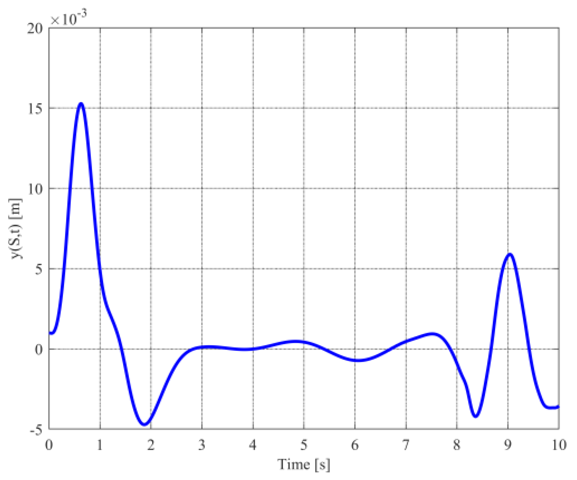
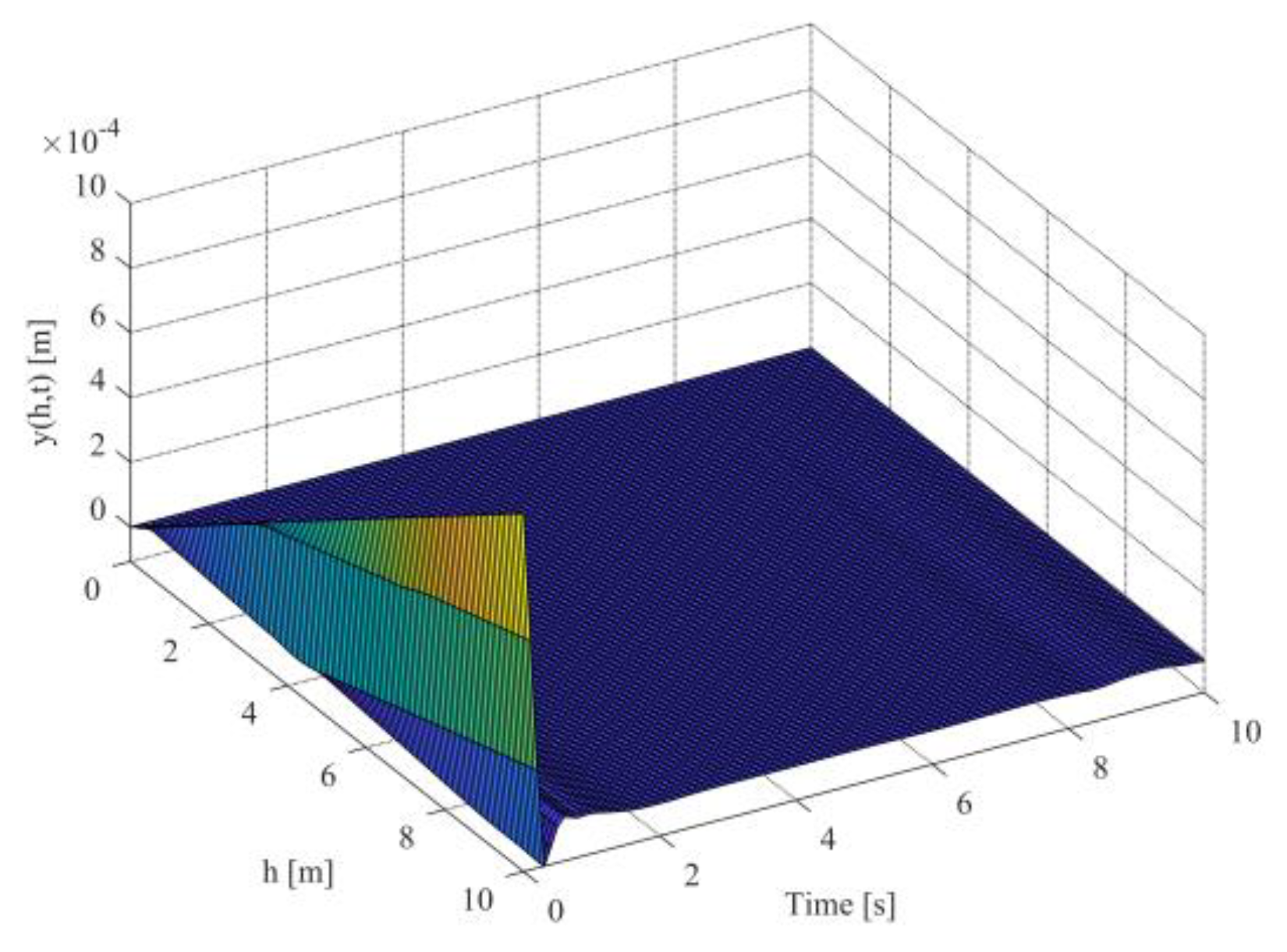
The three-dimensional vibration graph is shown in Figure 2, and the vibration image of $y(S,t)$ is given in Figure 3. From Figure 2 and Figure 3, we can clearly see that the belt system suffers from considerable vibration, which may lead to instability, and normal operation will be affected in practice.

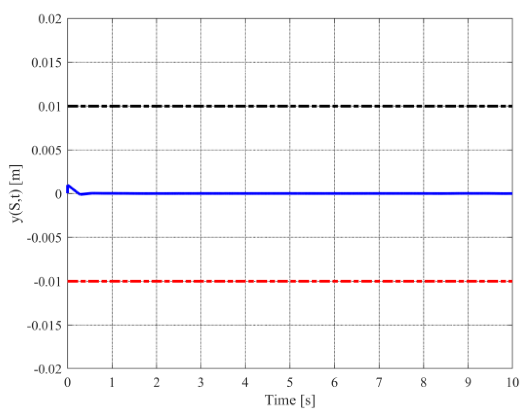
Considering the situation when $y_{ht}(S,t)$ can be directly used by the controller. Figure 4 describes the displacement of belt under the state feedback boundary controller $u$. It is obvious that the system becomes steady quickly. 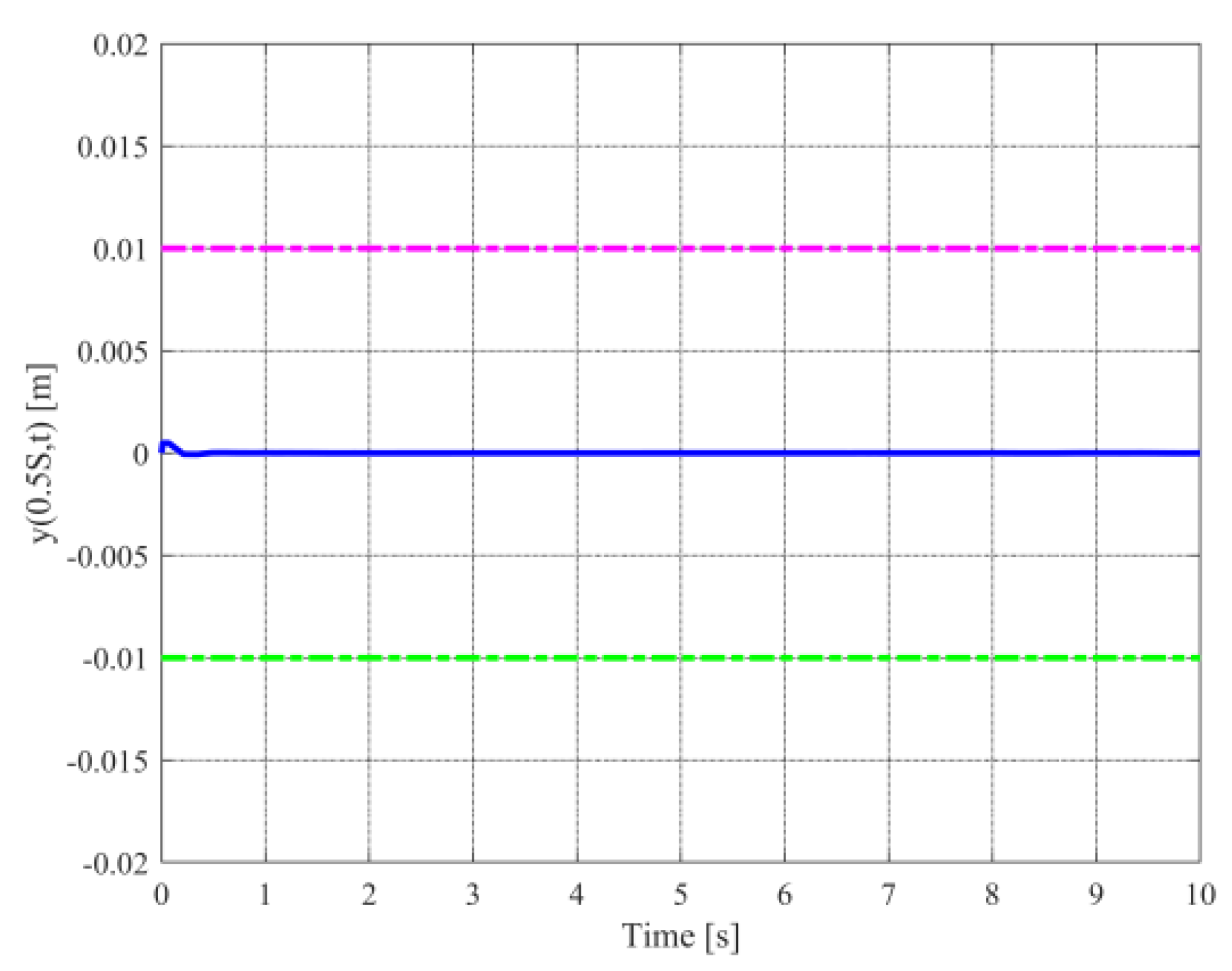Figure 5 expresses the corresponding trajectory of the boundary vibration $y\left(S,t\right)$, which implies that $\left|y\left(S,t\right)\right|<l_0$ holds all the time, i.e., the constraint conditions for $y\left(S,t\right)$ are satisfied. In order to further illustrate the control performance, we give the vibration curve at $h=5m$ in Figure 6. It is easy to see that the vibration is within a small neighborhood of the equilibrium position.

Considering the state $y_{ht}(S,t)$ cannot be directly used in the controller. In Figure 7, the system vibration map under the output feedback controller $u_0$ is given. It is concluded that although the state signal $y_{ht}(S,t)$ is unavailable, the system can also become stable through the output feedback controller $u_0$. The curve of the boundary vibration $y\left(S,t\right)$ is shown in Figure 8, from which we know that it meets the constraint conditions. Similarly, to further illustrate the control performance, we select the vibration image at $h=5$ m in Figure 9, which shows that the vibration at $h=5$ m is bounded and very small.

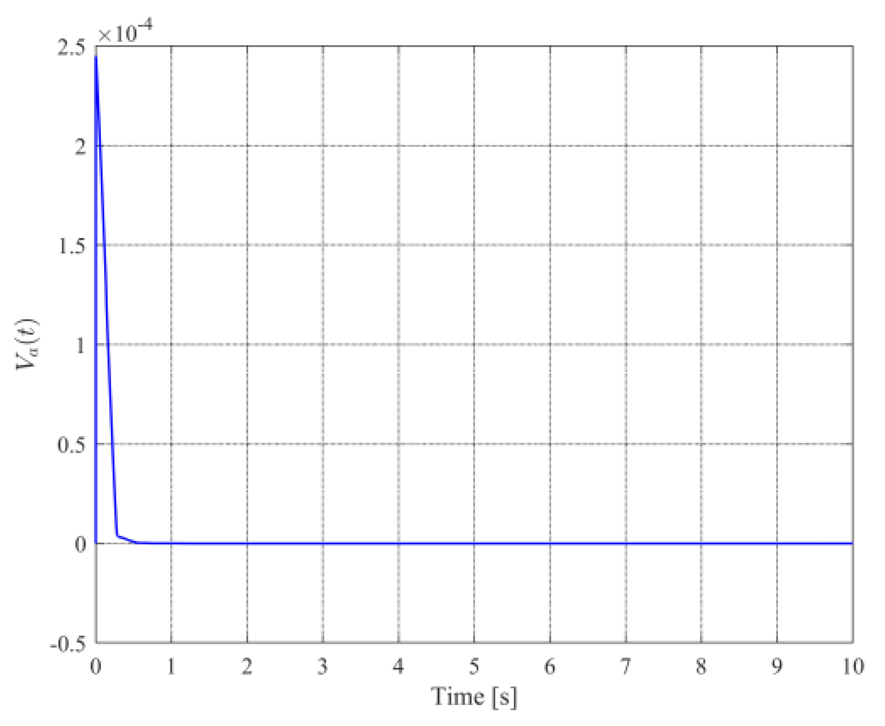
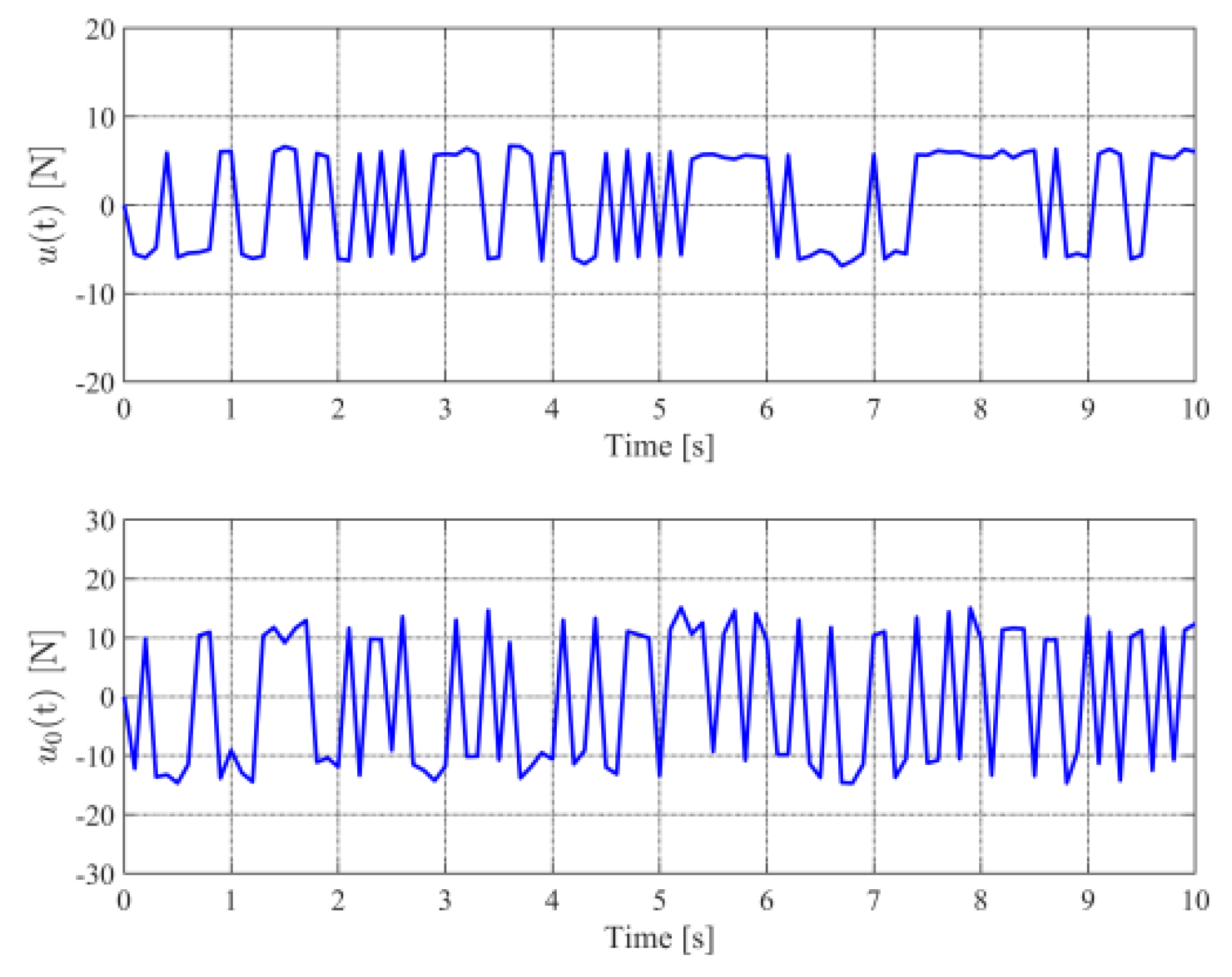
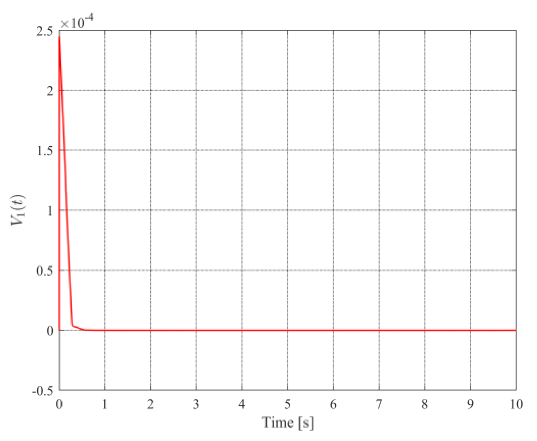
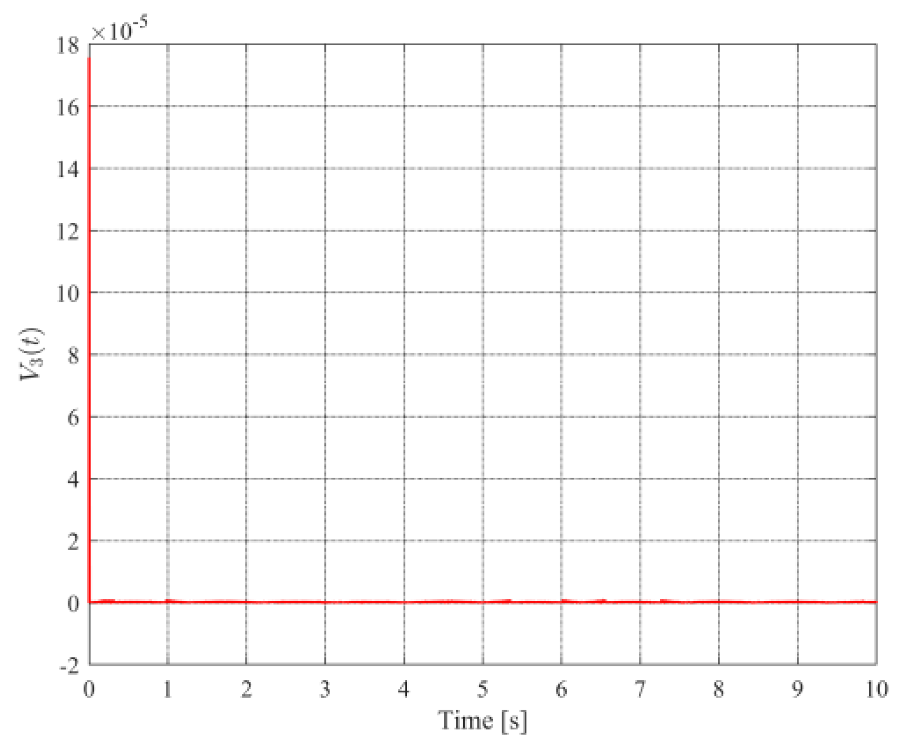
Figure 10 shows the error between the true and estimated values of state $x_2$. The error is small and bounded, which, to a certain extent, explains the effectiveness of the designed observer. Figure 11 describes the trajectories of two controllers, it can also clearly be seen that the two controllers are bounded. Further, for the Lyapunov function candidates constructed for the considered two cases, we show their trajectories over time with Figure 12, Figure 13, Figure 14, Figure 15, Figure 16, Figure 17, Figure 18 and Figure 19. It can be clearly seen that $V(t)$ and $V_0(t)$ are positive, definite, and bounded, thus indicating the suitability of our designed Lyapunov function candidates.

In conclusion, our designed state feedback and output feedback boundary control schemes can effectively deal with the system boundary vibration constraints and suppress the transverse vibration of the system, indicating that the two developed controllers stabilize the horizontal belt system with good performance.

5. Conclusions

In this paper, we deal with the boundary control problem for a horizontal band system with boundary vibration constraints. Firstly, we did not simplify or discretize the model of the system, so that we avoided problems such as the loss of the system signal caused by the simplification of the model. Secondly, in order to achieve the purpose of suppressing the transverse vibration of the system and ensuring that the system does not violate the boundary vibration limit during operation, we designed a state feedback control scheme and an output feedback control scheme for different cases of the system boundary signals. Specifically, a smooth logarithmic function was used to handle the system boundary constraint. When the system boundary signals could be used directly, a high-gain observer was used to estimate it. In addition, this paper mainly proved the boundedness of the system solution, and the existence and uniqueness of the solution of this closed-loop system was also proved. The interested reader is referred to [24]. Finally, we verified the effectiveness of the proposed controller using numerical simulations. In the next work, we will focus on studying various constraints for other flexible systems.

References

1. Dong, H.; Lu, C.; Yang, H. The finite volume WENO with Lax–Wendroff scheme for nonlinear system of Euler equations. Mathematics 2018, 6, 211. [Google Scholar] [CrossRef] [Green Version]
2. Wang, X.; Wang, H.; Zhao, J.; Xu, C.; Luo, Z.; Han, Q. Rigid-Flexible coupling dynamics modeling of spatial Crank-Slider mechanism based on absolute node coordinate formulation. Mathematics 2022, 10, 881. [Google Scholar] [CrossRef]
3. Malik, A.I.; Kim, B.S. A constrained production system involving production flexibility and carbon emissions. Mathematics 2020, 8, 275. [Google Scholar] [CrossRef] [Green Version]
4. Beltran-Carbajal, F.; Abundis-Fong, H.F.; Trujillo-Franco, L.G.; Yañez-Badillo, H.; Favela-Contreras, A.; Campos-Mercado, E. Online frequency estimation on a building-like structure using a nonlinear flexible dynamic vibration absorber. Mathematics 2022, 10, 708. [Google Scholar] [CrossRef]
5. How, B.V.; Ge, S.S.; Choo, Y.S. Active control of flexible marine risers. J. Sound Vib. 2009, 32, 758–776. [Google Scholar] [CrossRef]
6. Hao, J.; Wang, Z.; Yi, W.; Chen, Y.; Chen, J. Influence of the flexible tower on aeroelastic loads of the wind turbine. Appl. Sci 2021, 11, 8876. [Google Scholar] [CrossRef]
7. He, W.; Zhang, S. Control design for nonlinear flexible wings of a robotic aircraft. IEEE Trans. Control Syst. Technol. 2017, 25, 351–357. [Google Scholar] [CrossRef]
8. Liu, Z.J.; Liu, J.K. Adaptive boundary control of a flexible manipulator with input saturation. Int. J. Control 2016, 89, 1191–1202. [Google Scholar] [CrossRef]
9. Aoustin, Y.; Chevallereau, C. The singular perturbation control of a two-flexible-link robot. IEEE Int. Conf. Robot. Autom. 1993, 737–742. [Google Scholar]
10. Jiang, T.T.; Liu, J.K.; He, W. Boundary control for a flexible manipulator based on infinite dimensional disturbance observer. J. Sound Vib. 2015, 348, 1–14. [Google Scholar] [CrossRef]
11. Rahn, C.D. Mechatronic control of distributed noise and vibration-a Lyapunov approach. Meas. Sci. Technol. 2001, 39, 1664–1666. [Google Scholar] [CrossRef] [Green Version]
12. Meirovitch, L.; Baruh, H. On the problem of observation spillover in self-adjoint distributed systems. J. Optim. Theory Appl. 1983, 30, 269–291. [Google Scholar] [CrossRef]
13. Balas, M.J. Active control of flexible systems. J. Optim. Theory Appl. 1978, 25, 415–436. [Google Scholar] [CrossRef]
14. Paul, C.P.; Lai, C.L. Boundary control of an axially moving string via fuzzy sliding-mode control and fuzzy neural network methods. J. Sound Vib. 2003, 262, 795–813. [Google Scholar]
15. Shen, D.; Xu, J.X. An iterative learning control algorithm with gain adaptation for stochastic systems. IEEE Trans. Autom. Control 2020, 65, 1280–1287. [Google Scholar] [CrossRef]
16. Liu, Y.; Guo, F.; Zhao, Z.J. Boundary barrier-based control of a flexible riser system. IET Control Theory Appl. 2017, 11, 923–930. [Google Scholar] [CrossRef]
17. He, W.; Sun, C.; Ge, S.S. Top tension control of a flexible marine riser by using integral-barrier Lyapunov function. IEEE/ASME Trans. Mechatron. 2014, 20, 497–505. [Google Scholar] [CrossRef]
18. Dogan, M.; Morgul, O. Boundary control of a rotating shear beam with observer feedback. J. Vib. Control 2012, 18, 2257–2265. [Google Scholar] [CrossRef] [Green Version]
19. Tran, D.T.; Dao, H.V.; Dinh, T.Q. Output feedback control via linear extended state observer for an uncertain manipulator with output constraints and input dead-zone. Electronic 2020, 9, 1355. [Google Scholar] [CrossRef]
20. Yang, H.J.; Liu, J.K.; He, W. Distributed disturbance-observer-based vibration control for a flexible-link manipulator with output constraints. Sci. China Technol. Sci. 2018, 61, 1528–1536. [Google Scholar] [CrossRef]
21. Yang, H.; Liu, J. Observer design for a flexible-link manipulator with PDE model. J. Sound Vib. 2015, 34, 237–245. [Google Scholar] [CrossRef]
22. Yang, H.; Liu, J. Distributed piezoelectric vibration control for a flexible-link manipulator based on an observer in the form of partial differential equations. J. Sound Vib. 2016, 363, 77–96. [Google Scholar] [CrossRef]
23. Jin, F.F.; Guo, B.Z. Lyapunov approach to output feedback stabilization for the Euler–Bernoulli beam equation with boundary input disturbance. Automatica 2015, 52, 95–102. [Google Scholar] [CrossRef]
24. Zhao, Z.J.; Liu, Y.; Luo, F. Output feedback boundary control of an axially moving system with input saturation constraint. ISA Trans. 2017, 68, 22–32. [Google Scholar] [CrossRef] [PubMed]
25. Zhao, Z.J.; Liu, Y.; Luo, F. Adaptive boundary control of an axially moving belt system with high acceleration/deceleration. IET Control Theory Appl. 2016, 10, 1299–1306. [Google Scholar] [CrossRef]
26. Liu, Y.; Zhao, Z.J.; He, W. Boundary control of an axially moving accelerated/decelerated belt system. Int. J. Robust Nonlinear Control 2016, 26, 3849–3866. [Google Scholar] [CrossRef]
27. Liu, Y.; Zhao, Z.J.; He, W. Stabilization of an axially moving accelerated/decelerated system via an adaptive boundary control. ISA Trans. 2016, 64, 394–404. [Google Scholar] [CrossRef]
28. Sen, M.; Luo, N. Design of linear observers for a class of linear hybrid systems. Int. J. Syst. Sci. 2000, 31, 1077–1090. [Google Scholar] [CrossRef]
29. Manaa, I.; Barhoumi, N.; Msahli, F. Global stability analysis of switched nonlinear observers. Int. J. Autom. Comput. 2015, 12, 432–439. [Google Scholar] [CrossRef]
30. Wei, Y.L.; Jia, S.S.; Liu, K.M. A survey on anti-disturbance control of switched systems with input saturation. Syst. Sci. Control Eng. 2020, 8, 241–248. [Google Scholar] [CrossRef]
31. Zhao, Z.J.; Ma, Y.H.; Ren, Z.G. Vibration boundary control for a one-dimensional flexible beam system with restricted input. IEEE Access 2018, 6, 43336–43342. [Google Scholar] [CrossRef]
32. Rahn, C.D. Mechatronic Control of Distributed Noise and Vibration; Springer: New York, NY, USA, 2001. [Google Scholar]
33. Behtash, S. Robust output tracking for non-linear systems. Int. J. Control 1990, 51, 1381–1407. [Google Scholar] [CrossRef]
Figure 1. A schematic of horizontal belt transmission system.
Mathematics 10 01391 g001
Figure 2. The displacement of belt without control.
Mathematics 10 01391 g002
Figure 3. The boundary vibration y ( S , t ) without control.
Mathematics 10 01391 g003
Figure 4. The displacement of belt under the state feedback boundary controller.
Mathematics 10 01391 g004
Figure 5. The boundary vibration y ( S , t ) under the state feedback controller: l 0 (black line), y ( S , t ) (blue line), l 0 (red line).
Mathematics 10 01391 g005
Figure 6. The vibration y ( 0.5 S , t ) under the state feedback controller: l 0 (purple line), y ( 0.5 S , t ) (blue line), l 0 (green line).
Mathematics 10 01391 g006
Figure 7. The displacement of belt under the output feedback boundary control.
Mathematics 10 01391 g007
Figure 8. The boundary vibration y ( S , t ) under the output feedback control: l 0 (black line), y ( S , t ) (blue line), l 0 (red line).
Mathematics 10 01391 g008
Figure 9. The vibration y ( 0.5 S , t ) under the output feedback controller: l 0 (purple line), y ( 0.5 S , t ) (blue line), l 0 (green line).
Mathematics 10 01391 g009
Figure 10. The curve of estimation error x ˜ 2 ( t ) .
Mathematics 10 01391 g010
Figure 11. The trajectory of controllers u and u 0 .
Mathematics 10 01391 g011
Figure 12. The trajectory of V a ( t ) .
Mathematics 10 01391 g012
Figure 13. The trajectory of V b ( t ) .
Mathematics 10 01391 g013
Figure 14. The trajectory of V c ( t ) .
Mathematics 10 01391 g014
Figure 15. The trajectory of V ( t ) .
Mathematics 10 01391 g015
Figure 16. The trajectory of V 1 ( t ) .
Mathematics 10 01391 g016
Figure 17. The trajectory of V 2 ( t ) .
Mathematics 10 01391 g017
Figure 18. The trajectory of V 3 ( t ) .
Mathematics 10 01391 g018
Figure 19. The trajectory of V 0 ( t ) .
Mathematics 10 01391 g019