Optimization of Genetic Algorithm through Use of Back Propagation Neural Network in Forecasting Smooth Wall Blasting Parameters

Abstract

With the continuous development in drilling and blasting technology, smooth wall blasting (SWB) has been widely applied in tunnel construction to ensure the smoothness of tunnel profile, diminish overbreak and underbreak, and preserve the tunnel’s interior design shape. However, the complexity of the actual engineering environment and the deficiency of current optimization theories have posed certain challenges to the optimization of SWB parameters under arbitrary geological conditions, on the premise that certain control targets are satisfied. Against the above issue, a genetic algorithm (GA) and back propagation (BP) neural network-based computational model for SWB design parameter optimization is proposed. This computational model can comprehensively reflect the relation among geological conditions, design parameters, and results by training and testing the 285 collected sets of test data samples at different conditions. Moreover, it automatically searches optimal blasting design parameters through the control of SWB targets to acquire the optimal design parameters based on specific geological conditions of surrounding rocks and under the specified control targets. When the optimization algorithm is compared with other current optimization algorithms, it is shown that this algorithm has certain computational superiority over the existing models. When the optimized results are applied in practical engineering, it is shown that in overall consideration of the geological conditions, control targets, and other influencing factors, the proposed GA_BP-based model for SWB parameter optimization has high feasibility and reliability, and that its usage can be generalized to analogous tunneling works.

1. Introduction

Drilling and blasting method is the main technique for tunnel construction [1]. With the progress in construction techniques, the SWB technique has been widely accepted in drilling and blasting operations. SWB can effectively control the blasting effect, and hence diminish overbreak and underbreak, keep the tunnel’s rocky wall smooth, and further maintain the stability of surrounding rocks, lessen the supporting workload, reduce the support materials and engineering costs required, and shorten the construction period [2]. The core issue of SWB lies in the control of overbreak and underbreak [3]. Mahtab [4] believes that the combination of traditional blasting methods with simulation technology can assist in the further evaluation of overbreak and underbreak through the tunnel while the tunnel is drilled and blasted forward; the research outcomes can predict the total overbreak and underbreak through the tunnel and further define the confidence interval of the probability of the region where overbreak and underbreak appear. With further development in computer technology, the machine learning method has been widely accepted and used by more and more scholars to predict overbreak and underbreak in surface blasting operations [5,6]. Likewise, the theoretical and experimental studies on overbreak and underbreak have also achieved new breakthroughs [7,8,9] and explained macroscopic and microscopic reasons for overbreak and underbreak [10,11,12].

According to research findings, numerous parameters are accountable for the SWB effect, including the physical and mechanical properties of mineral rocks (such as compressive and tensile strengths, joint development degree, etc.), blasting design parameters (such as hole pitch, array pitch, blast hole depth, charge concentration, etc.), and evaluation indexes of blasting effect (such as average linear overbreak, average linear underbreak, etc.). Therefore, the selection of influencing factors for SWB is a multilevel, multifactor, multigoal complex decision-making process, with extremely convoluted uncertainty and nonlinear relations between blasting parameters and results [13,14]. However, in the current stage, SWB parameters are determined by the mere empirical method or in mere consideration of one or more simple factors; thus, blasting design parameters are extremely subjective and random [15]. The optimization of SWB parameters is always a challenge under any geological condition with certain control targets (blasting construction targets) [16].

In practical engineering, especially underground engineering, field test data are typically finite and discrete due to a myriad of limits of the field environment [17]. A mainstream solution to the global optimization problem with finite and discrete samples in underground engineering is the support vector machine (SVM) [18,19] and artificial neural network (ANN) [20,21]. The core of SVM is the minimum structural risk such that it has small sample demand and low fitting precision. Therefore, it is more applicable in parameter optimization problems with small numbers of parameters and samples. However, with the continuous development in blasting technology, more and more influencing factors need to be taken into consideration, and higher and higher requirement is raised on the precision of design parameters. Therefore, the minimum empirical risk-based neural network technology has received more attention and is more commonly used [22,23].

This study proposes an improved neural network algorithm: the GA_BP neural network algorithm, which has optimized the neural network’s initial weights and thresholds, enhanced the fitting precision of BP neural network under small and medium sample sizes, and collected the SWB parameters from other engineering projects under different geological conditions. With the 145 sets of measured data of SWB including the above data as the training samples, and with the 20 sets of field test data in the East Tianshan tunneling project in Xinjiang as the test samples, the nonlinear mapping relation between blasting design parameters and blasting results is obtained through GA_BP neural network fitting. On this base, the blasting effect parameters and parts of the blasting design parameters are controlled as per the practical engineering requirements, and the optimal solutions of blasting design parameters under the control conditions are searched for automatically, so as to achieve the optimization of the design parameters.

In the work of this paper, the coupling algorithm for the GA and BP neural network has been described in Section 2. Section 3 introduces the computation flow of the GA_BP neural network algorithm-based SWB parameter optimization model. Section 4 analyzes, evaluates, and verifies the optimized results in combination with an engineering case. Section 5 is the conclusion.

2. Methods

The traditional BP neural network is prone to parameter underfitting due to improper selection of initial parameters while training with small and medium samples. To address this problem, the genetic algorithm (GA) is combined with the BP neural network. The preferable weights and thresholds of the initial network are obtained by GA, and thus the fitting precision of the BP neural network is improved [24,25,26,27].

2.1. Genetic Algorithm (GA)

The implementation of GA includes the following 5 steps: [28]

(a)

Population initialization.

Individuals are encoded by the real coding method. Each individual is a real string composed of 4 components: weight of connection between the input layer and the hidden layer, threshold of the hidden layer, weight of connection between the hidden layer and the output layer, and threshold of the output layer. The individuals comprise all weights and thresholds of the neural network. Provided that the network structure is known, a network with a definite mapping structure, number of nodes, weights, and thresholds can be constructed.

(b)

Fitness function.

According to the initial values of the BP neural network obtained by the individuals, the system output is predicted after training the BP neural network using the training data, and the absolute value of the error and the variance E between the predicted output and the expected output as individual fitness F is taken, as calculated by the Equation (1):

$$F=k({\displaystyle \sum _{i=1}^{n}abs(y_i-o_i))}$$

(1)

where n is the number of the network’s output nodes; y_i is the expected output of the ith node of the BP neural network; o_i is the predicted output of the ith node; k is the coefficient for normalization; in this paper, k = 1.

(c)

Selection operation.

The selection operation in GA is based on the selection strategy of fitness proportion. The selection probability, p_i, of each individual i is:

$$f_i=k/F_i$$

(2)

$$p_i=\frac{f_i}{{\displaystyle \sum _{j=1}^N{f}_j}}$$

(3)

where F_i is the fitness value of individual i. As it is preferred that fitness be as small as possible, the fitness value shall be inverted prior to individual selection. k is the coefficient with the same value as Formula (1); N is the number of individuals in the population.

(d)

Crossover operation.

As individuals are encoded by real coding, the crossover operation is performed by a real number crossover method. The crossover operation on the kth chromosome a_k with the lth chromosome a_l at position j is performed by the following method:

$$\begin{array}{l}{a}_{kj}=a_{kj}(1-b)+a_{lj}b\\ a_{lj}=a_{ij}(1-b)+a_{kj}b\end{array}$$

(4)

where: b is a random number within (0, 1).

(f)

Mutation operation.

The jth gene of the ith individual, a_ij, is selected to undergo mutation, as operated by the following method:

$$\begin{array}{l}{a}_{ij}=a_{ij}+\left(a_{ij}-a_{\max }\right)\times f(g)\begin{array}{cc}& \end{array}r>0.5\\ a_{ij}=a_{ij}+\left(a_{\min }-a_{ij}\right)\times f(g)\begin{array}{cc}& \end{array}r\le 0.5\end{array}$$

(5)

where a_max is the upper bound to gene a_ij; a_min is the lower bound to gene a_ij; $f\left(g\right)=r_2{\left(1-g/G_{\max }\right)}^2$; r₂ is a random number; g is the count up to the current iteration; G_max is the maximum evolution count; r is a random number used to judge the mutation operation within (0, 1), which is automatically generated when selecting a_ij.

2.2. BP Neural Network

The BP neural network is a multilayer feedforward neural network that can be regarded as a nonlinear function, whose independent and dependent variables are the network’s input value and predicted value, respectively. When the number of input nodes is n and the number of output nodes is m, the BP neural network expresses the function mapping relation from the n independent variables to the m dependent variables. The BP neural network shall be trained prior to prediction so that it is endowed with associative memory and predictive ability. The training process of BP neural network includes the following 7 steps: [29]

(a)

Network initialization.

According to the system’s input and output sequences (X, Y), determine the number of nodes, n, at the network’s input layer, the number of nodes, l, at the hidden layer, the number of nodes, m, at the output layer, initialize the weights w_ij and w_jk of connections between neurons at the input layer, hidden layer, and the output layer, respectively, and the threshold, a, of the hidden layer and the threshold, b, of the output layer, and give the learning rate and the neuron excitation function.

• (b) Hidden layer output calculation.

According to the input variable X, weight w_ij of connection between the input layer and the hidden layer, and threshold a of the hidden layer, calculate the hidden layer output H.

$$H_j=f\left({\displaystyle \sum _{i=1}^n{w}_{ij}{x}_i-a_j}\right)\begin{array}{cc}& \end{array}j=1,2,\dots ,l$$

(6)

where l is the number of nodes at the hidden layer; f is the excitation function of the hidden layer, which can be expressed in many ways. Here, the excitation function is selected as:

$$f\left(x\right)=\frac{1}{1+e^{-x}}$$

(7)

• (c) Output layer output calculation.

According to the hidden layer output H and the weight of connection w_ij and threshold b, calculate the predicted output O of the BP neural network.

$$O_k={\displaystyle \sum _{j=1}^l{H}_j}{w}_{jk}-b_k\begin{array}{cc}& \end{array}k=1,2,\dots ,m$$

(8)

• (d) Error calculation.

According to the network’s predicted output O and expected output Y, calculate the network’s predicted error e.

$$e_k=Y_k-O_k\begin{array}{cc}& \end{array}k=1,2,\dots ,m$$

(9)

• (e) Weights update.

According to the network’s predicted error e, update the weights w_ij and w_jk of network connections.

$$w_{ij}=w_{ij}+\eta H_j\left(1-H_j\right)x\left(i\right){\displaystyle \sum _{k=1}^m{w}_{jk}{e}_k}\begin{array}{cc}& \end{array}i=1,2,\dots ,n;j=1,2,\dots ,l$$

(10)

$$w_{jk}=w_{jk}+\eta H_j{e}_k\begin{array}{cc}& \end{array}j=1,2,\dots ,l;k=1,2,\dots ,m$$

(11)

where η is the learning rate.

• (f) Thresholds update.

According to the network’s predicted error e, update the thresholds a and b of network nodes.

$$a_j=a_j+\eta H_j\left(1-H_j\right)x\left(i\right){\displaystyle \sum _{k=1}^m{w}_{jk}{e}_k}\begin{array}{cc}& \end{array}j=1,2,\dots ,l$$

(12)

$$b_k=b_k+e_k\begin{array}{cc}& \end{array}k=1,2,\dots ,m$$

(13)

• (g) Judge whether the algorithm iterations come to an end; if not, return to Step (b).

2.3. GA_BP Neural Network

The parameter fitting calculation of the GA_BP neural network falls into two components: the BP neural network and GA optimization. The calculation flowchart is shown in Figure 1.

Where the BP neural network is composed of two parts: One is the part of the BP neural network structure determination, namely to determine the results of the BP neural network, and thereby the length of GA individuals, according to the number of input and output parameters of the fitting function; the other is the part of the BP neural network parameter fitting, which is responsible for fitting the neural network’s input and output parameters, determining the nonlinear relations between parameters, and predicting the function output after network training. The GA optimization component uses the weights and thresholds of the genetic optimization algorithm of the BP neural network. Each individual in the population comprises all weights and thresholds of a network. Individuals’ fitness is calculated via the fitness function, in order for the genetic algorithm to find the individual with the optimal fitness value through selection, crossover, and mutation operations, and thus to optimize the initial weights and thresholds of the BP neural network. The concrete procedure of GA_BP neural network goes as follows:

(a) Determine the input and output parameters of GA_BP neural network; (b) initialize the weights and thresholds between the initial parameters of the BP neural network; (c) optimize the above weights and thresholds by GA and select the optimal ones; (d) fit the input and output parameters of GA_BP neural network; (e) error test as to whether the requirement is met, if yes end the calculation, or else return to Step (c).

3. Optimization Model

3.1. Parameter Optimization

The calculation for the SWB parameter optimization is to determine the nonlinear relations between input parameters and output parameters by fitting all these parameters via the GA_BP neural network, and to implement the prediction of the output results under the condition of input parameters; next, through the control of the output results, it automates the optimization model to search for the optimal solutions among the input parameters. The calculation process falls into two parts: One is the fitting of GA_BP neural network parameters, and the other is the calculation for parameter optimization. The concrete calculation model is shown in Figure 2.

The concrete steps of calculation for the SWB parameter optimization go as follows:

• Initialize the GA_BP neural network and determine the optimal neural network parameters;
• Fit the input parameters and output parameters of SWB among the training samples of the GA_BP neural network;
• After fitting the parameters of the GA_BP neural network, conduct an error analysis into the GA_BP neural network using the test samples. If the requirement is met, go to the next step, else return to the first step and modify the basic parameters of the neural network;
• When the fitting results meet the requirement of test error, the nonlinear relations between the input and output parameters are reflected, and thus the prediction of results is implemented;
• According to the purpose of practical engineering and the parameter design requirement (input parameter control), determine the calculation parameters when the event counter P = 1;
• Try figuring out the SWB calculation results under the feasible condition when the event counter P = 1, using the nonlinear relations reflected in the GA_BP neural network.
• After going through the case when the event counter P = 1, determine the calculation parameters when the event counter P = 2, and return to the previous step for calculation until covering all event counters for P = P + 1;
• Control the calculation results and thus automatically search for the optimal values of them under this trial condition, so as to derive the optimal design parameters by inversion and implement the optimization of SWB design parameters.

3.2. Parameters

In practical tunneling, SWB involves numerous data. Taking the parameters into consideration of the calculation model for SWB parameter optimization is bound to the problems of data redundancy and computational complexity. Therefore, it is necessary to screen the important parameters in SWB and perform the corresponding simplification of the concrete fitting parameters. In general, the SWB effect is subject mainly to geological conditions and blasting parameters. Accordingly, the selected parameters should include factors in three aspects: geological conditions, blasting design parameters, and blasting result parameters. Considering the practical engineering application, and for the convenience of the uniform measurement of test data, the SWB parameters are simplified with overall consideration of the blasting design standard and scholars’ research outcomes [8,30,31]. Figure 3 is a schematic diagram of the SWB design parameters. Figure 4 is a schematic diagram for the calculation of average linear overbreak and underbreak.

Average overbreak and underbreak are calculated by the formulae:

$$S_c=\frac{S_{c1}+S_{c2}+\dots +S_{cn}}{I_{c1}+I_{c2}+\dots +I_{cn}}$$

for average linear overbreak, and:

$$S_q=\frac{S_{q1}+S_{q2}+\dots +S_{qn}}{I_{q1}+I_{q2}+\dots +I_{qn}}$$

for average linear underbreak, where I_c and I_q correspond, respectively, to the arclength corresponding to each overbreak area and underbreak area.

For optimization calculation, the input parameters are the ones that affect the blasting results, whereas the output parameters are the blasting results. Moreover, in practical engineering, due to the influences of geological conditions, boring equipment, and tunneling purpose, the parameters already have fixed values or designed values and cannot or need not be optimized further. Therefore, the core purpose of SWB parameter optimization is to search for the optimal solutions of spacing between lines of least resistance W, auxiliary hole pitch E_b, and ambient hole pitch E_a, under the condition of controlling the average linear overbreak and average linear underbreak.

3.3. Determination of GA_BP Neural Network Topology and Basic Parameters

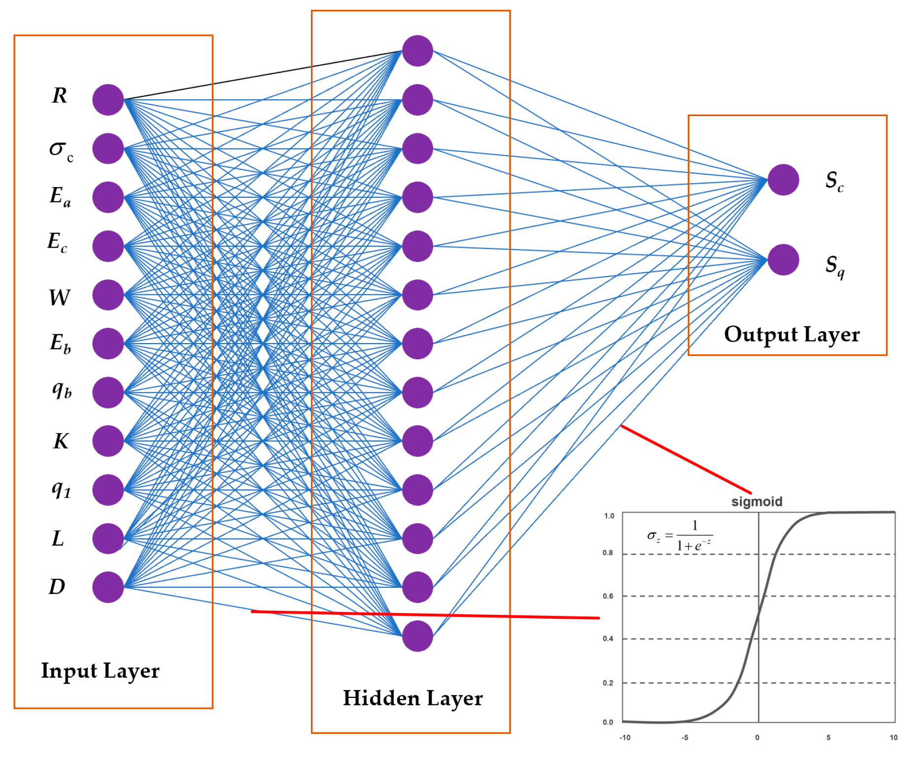
Through the above description, the number of input parameters of the GA_BP neural network can be determined to be 11, whereas the number of output parameters is 2. The neural network adopts a three-layer topological structure. The excitation function is selected as a sigmoid function.

Generally, the number of nodes in the hidden layer is calculated by the following empirical formulas [29]:

$$l<\sqrt{mn}$$

(14)

$$l<\sqrt{\left(m+n\right)}+a$$

(15)

$$l={\log }_{2}n$$

(16)

where n is the number of input layer nodes, l is the number of hidden layer nodes, m is the number of output layer nodes, and a is a constant between 0 and 10.

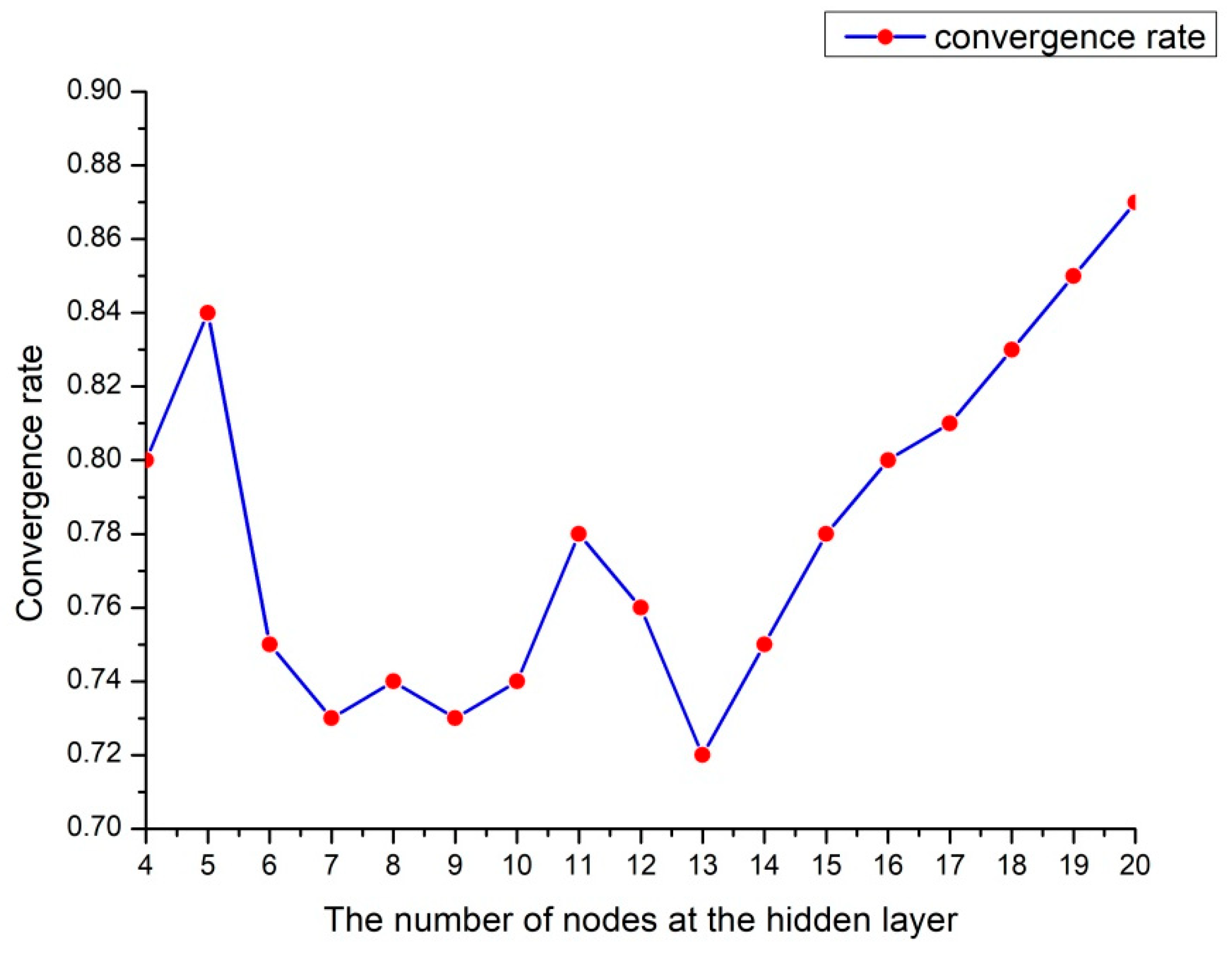
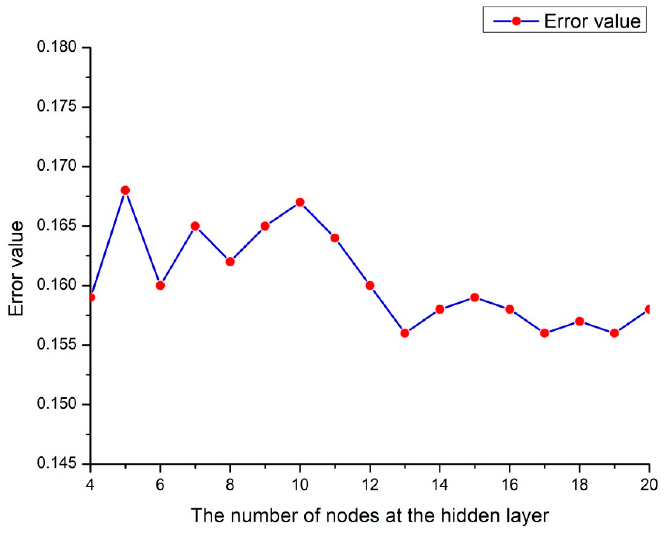
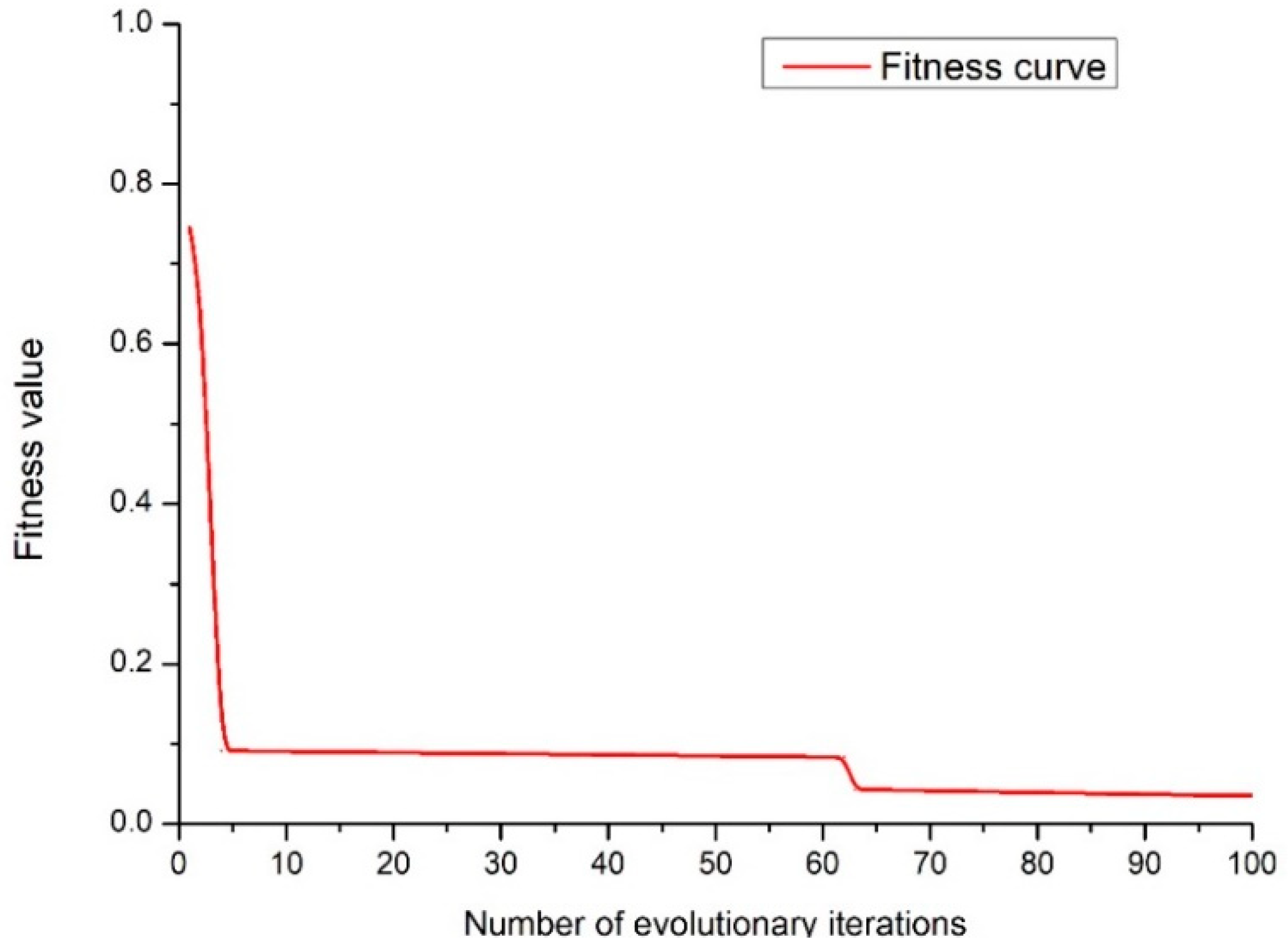
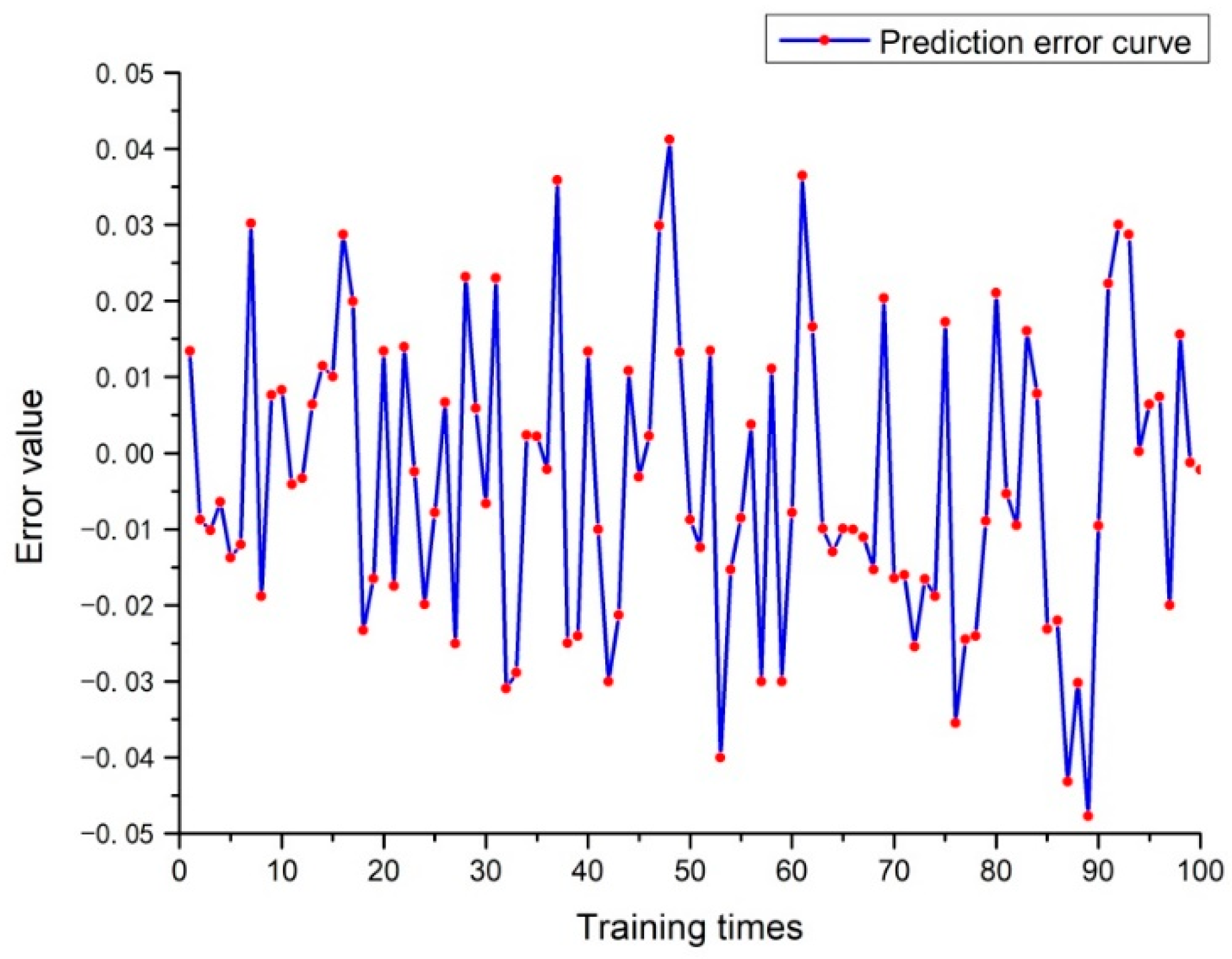
In this paper, the number of nodes in the input layer is n = 11 and the number of nodes in the output layer is m = 2. Therefore, according to the above formula, it is considered that the value range of l is between 4 and 20. Figure 5 and Figure 6 show the convergence speed during sample training and the error rate after sample fitting under different hidden layer nodes during trial calculation. Considering the results of Figure 1 and Figure 2, it is most reasonable to set the number of nodes of the hidden layer as l = 13.

Relevant references [32,33], are selected to determine the network’s initial basic parameters: The number of nodes at the hidden layer of GA_BP neural network is 13, with 11 × 13 + 2 × 13 = 169 weights and 13 + 2 = 15 thresholds; individual encoding length in GA is 169 + 15 = 184, population size is 20, evolution count is 100, crossover probability is 0.94, and mutation probability is 0.2. The final GA_BP neural network topology is shown in Figure 7.

3.4. Control Targets of SWB Parameter Optimization

The purpose of parameter optimization is to search for the optimal results. SWB involves numerous parameters, and, without a unique evaluation index of the blasting results, the evaluation is a multitask and multipurpose problem. At the current stage, the multitask and multipurpose optimization using neural network is implemented mainly by two methods: One is to figure out the multiple goals into mutually independent target solutions by the method of Pareto solutions, and the other is to turn the multiple goals into single goals by some calculation model. Combining the practical engineering, the two target parameters, the average linear overbreak and average linear underbreak, are difficult to become mutually independent target solutions. Therefore, the latter approach can be more effective. Moreover, the optimal solutions for the results of SWB typically need to meet two requirements: One is that the tunnel profile shall be as smooth as possible; the other is that the contour line of the practically blasted tunnel shall be as designed as possible. Therefore, reflected in the calculation model for optimization, the control targets of the output parameters are:

• The minimum of “average linear overbreak S_c + average linear underbreak S_q”;
• The minimum of average linear overbreak S_c.

4. Engineering Case

4.1. Project Overview

This paper relies on the East Tianshan tunneling project for the Barkol-Hami (first-class) highway G575, which is located in the area of Hami, Xinjiang. The two-way separated superlong tunnel covers a full length of 11.767 km of the sinistral tunnel and a full length of 11.776 km of the dextral tunnel; the maximum burial depth is 1225 m and the average burial depth is 706 m. Near the tunnel, one can find the typical western mountainous area with obvious underwater seepage. Affected by the burial depth and seepage, the overall strength of the tunnel’s surrounding rocks is low, and some construction sections are even vulnerable to the gushing of a large amount of underground water after being tunneled. The schematic diagram of tunnel construction is shown in Figure 8, and the schematic diagram of the project overview is shown in Figure 9.

4.2. Fitting Parameter Training of GA_BP Neural Network

4.2.1. Sample Collection

While 20 sets of SWB test data are collected from this project, 265 sets of the SWB test data are also collected from other tunneling projects. Figure 10 provides the sources of other SWB data. The input and output parameters of SWB are fitted with the 265 sets of data from other projects as the training samples of the GA_BP neural network and the 20 sets of field test data as the test samples.

According to the BQ method in the “Standard for Engineering Classification of Rock Masses” (GB 50218-94) of China and the BQ-RMR relation in (17), the parameter surrounding rock rank pertains to geological conditions among the sample data. Limited by space, this paper only displays the surrounding rock mass ranks under preliminary investigation in the Xinjiang-based project, as shown in

Table 1. Surrounding rock mass ranks under preliminary investigation.

Surrounding rock mass rank	BQ	Ⅴ	Ⅳ
	RMR	Ⅴ	Ⅳ
Length (km)/percentage (%)	Sinistral Tunnel	6.31/54	5.46/46
	Dextral Tunnel	6.88/58	4.89/42

.

$$\mathrm{RMR}=\left(\mathrm{BQ}-80.786\right)/6.0943$$

(17)

Still limited by space, only the 20 sets of blasting test sample data in the Xinjiang-based project for testing the fitting precision of the GA_BP neural network are presented in

Table 2. Test sample parameter list.

Order	Input Parameters											Output Parameters
No.	R	σc/MPa	Ec/mm	Ea/cm	Eb/cm	W/cm	qb/kg	K	ql	L/m	D/mm	Sc/cm	Sq/cm
1	4	37.93	12	50.1	73.3	45.4	1.8	1.5	0.25	4	48	3.6	–1.2
2	4	41.22	14	54.2	85	57	1.8	1.5	0.25	4	48	2.1	–7.8
3	4	38.36	12	53.9	79.4	86.7	1.8	1.5	0.25	4	48	0.9	–3.9
4	4	48.2	17	46.3	84.2	90.5	1.8	1.5	0.25	4	48	1.1	–4.2
5	4	44.6	16	56.7	71	68.2	1.8	1.5	0.25	4	48	6.9	–1.2
6	4	36.7	21	54.2	102	73.1	1.8	1.5	0.25	4	48	6.3	–1
7	5	26.6	41	65.1	145.1	55.6	1.8	1.5	0.2	4	48	1.2	–25.7
8	5	38.54	17	54.9	132.4	48.1	1.8	1.5	0.2	4	48	15.1	–1.4
9	5	36.78	34	59.2	102.5	52.5	1.8	1.5	0.2	4	48	1.7	–9.6
10	5	33.25	14	44.5	75.5	43.2	1.8	1.5	0.2	4	48	4.65	–1
11	5	38.34	42	60.1	90.6	70.1	1.8	1.5	0.2	4	48	15.2	–1.4
12	5	30.24	18	56.4	76.3	49.4	1.8	1.5	0.2	4	48	16.7	–1.7
13	5	28.71	11	56.5	86.4	50.1	1.8	1.5	0.2	4	48	19.4	–2.3
14	5	29.95	30	42.4	94.5	50.7	1.8	1.5	0.2	4	48	1.5	–15.3
15	5	25.75	26	57.3	123.1	62.8	1.8	1.5	0.2	4	48	1.9	–16.7
16	4	30.6	24	60.2	122.7	51	1.8	1.5	0.25	4	48	2.6	–17.5
17	4	31.4	23	76.4	148.3	47.3	1.8	1.5	0.25	4	48	2.7	–22.8
18	4	33.1	36	77.1	117.4	43.6	1.8	1.5	0.25	4	48	4.6	–21.5
19	4	34.3	38	78.9	120.1	46.3	1.8	1.5	0.25	4	48	3.2	–20.6
20	4	33.7	30	83.3	114.7	50.2	1.8	1.5	0.25	4	48	1.8	–18.2

, where the average overbreak is expressed in positive values and the average underbreak is expressed in negative values.

4.2.2. Sample Training Test

GA_BP neural network is used to train and test the above-collected samples. Figure 11 presents the fitness curves of the GA-optimized initial parameters of the BP neural network. Figure 12 presents the overall prediction error curves at distinct iteration counts when GA_BP neural network is fitting the input and output parameters of SWB. From Figure 11 and Figure 12, both the fitting precision and error can meet the practical requirements when the GA_BP neural network is fitting the input and output parameters of SWB, without the problem of underfitting or overfitting, and the nonlinear relations between input and output parameters of SWB can be achieved satisfactorily, hence the prediction of SWB results can be implemented.

4.2.3. The Accuracy of the Prediction in Both Training and Testing Data

Table 3. The accuracy of the prediction in training data.

No.	Overbreak/cm			Underbreak/cm
	Measured Value	Predicted Value	Error Rate	Measured Value	Predicted Value	Error Rate
1	7.8	7.752	0.62%	–6.3	–6.115	2.94%
2	2.0	2.121	6.05%	–7.3	–7.725	5.82%
3	6.7	6.862	2.42%	–4.7	–4.823	2.62%
4	6.4	6.301	1.55%	–5.1	–5.341	4.73%
5	5.1	5.005	1.86%	–6.1	–6.198	1.61%
6	2.9	2.774	4.34%	–6.7	–7.033	4.97%
7	3.4	3.331	2.03%	–2.0	–1.887	5.65%
8	5.8	5.255	9.40%	–4.5	–4.411	1.98%
9	8.7	8.543	1.80%	–8.0	–8.431	5.39%
10	7.7	7.561	1.81%	–9.9	–10.323	4.27%
11	5.2	5.011	3.63%	–2.8	–2.704	3.43%
12	7.2	7.588	5.39%	–5.6	–5.719	2.13%
13	9.9	9.562	3.41%	–5.1	–5.373	5.35%
14	4.7	4.471	4.87%	–2.8	–2.567	8.32%
15	8.2	8.658	5.59%	–4.3	–4.511	4.91%
16	5.3	5.523	4.21%	–7.2	–7.846	8.97%
17	3.9	3.658	6.21%	–5.7	–5.246	7.96%
18	7.3	7.521	3.03%	–4.2	–4.299	2.36%
19	3.8	3.93	3.42%	–2.2	–2.353	6.95%
20	8.8	8.995	2.22%	–6.1	–6.002	1.61%

and

Table 4. The accuracy of the prediction in testing data.

No.	Overbreak/cm			Underbreak/cm
	Measured Value	Predicted Value	Error Rate	Measured Value	Predicted Value	Error Rate
1	3.6	3.727	3.53%	–1.2	–1.265	5.42%
2	2.1	2.247	7.00%	–7.8	–7.621	2.29%
3	0.9	0.891	1.00%	–3.9	–3.844	1.44%
4	1.1	1.205	9.55%	–4.2	–4.141	1.40%
5	6.9	6.841	0.86%	–1.2	–1.114	7.17%
6	6.3	6.424	1.97%	–1	–1.045	4.50%
7	1.2	1.147	4.42%	–25.7	–24.876	3.21%
8	15.1	15.237	0.91%	–1.4	–1.412	0.86%
9	1.7	1.553	8.65%	–9.6	–9.613	0.14%
10	4.6	4.631	0.67%	–1	–1.023	2.30%
11	15.2	15.041	1.05%	–1.4	–1.404	0.29%
12	16.7	16.524	1.05%	–1.7	–1.712	0.71%
13	19.4	19.502	0.53%	–2.3	–2.323	1.00%
14	1.5	1.375	8.33%	–15.3	–15.421	0.79%
15	1.9	1.854	2.42%	–16.7	–16.521	1.07%
16	2.6	2.429	6.58%	–17.5	–17.323	1.01%
17	2.7	2.601	3.67%	–22.8	–22.651	0.65%
18	4.6	4.509	1.98%	–21.5	–21.212	1.34%
19	3.2	3.331	4.09%	–20.6	–20.412	0.91%
20	1.8	1.851	2.83%	–18.2	–18.023	0.97%

list the measured value, predicted value, and error rates for 20 sets of training data and 20 sets of testing data. It can be considered that, whether it is training data or test data, the error between the predicted value and the measured value is within 10%. Considering drilling work, this 10% error can be neglected. In general, the accuracy of the prediction meets the actual engineering requirements.

4.3. Results and Analysis of SWB Parameter Optimization Calculation

4.3.1. Parameter Input for Optimization Calculation

After the prediction of blasting results is implemented using the GA_BP neural network to complete SWB parameter fitting, the SWB design parameters can be optimized by controlling the predicted blasting results. Relying on the practical engineering project, this paper has designed five sets of different input parameters, among which the fixed parameters are shown in

Table 5. SWB involved fixed parameters in practical engineering.

No.	R	${\mathit{\sigma }}_{\mathbf{c}}/\mathbf{MPa}$	Ec/mm	qb/kg	K	q1	L/m	D/mm
1	4	42.34	20	1.8	1.5	0.25	4	48
2	4	55.27	20	1.8	1.5	0.25	4	48
3	4	48.45	20	1.8	1.5	0.25	4	48
4	5	38.12	20	1.8	1.5	0.2	4	48
5	5	36.94	20	1.8	1.5	0.2	4	48

, and the ranges of values of the parameters to be optimized are shown in

Table 6. Ranges of the parameters to be optimized.

Parameter	Ea/cm	W/cm	Eb/cm
Range	40~90	40~90	70~120

. As the values of W, E_b, and E_a are of little significance below the mm level in practical engineering, the parameters are optimized only at the cm level.

4.3.2. Optimization Calculation Results and Engineering Application

Table 7. Optimization calculation results.

No.	Ea/cm	W/cm	Eb/cm	Predicted Overbreak/cm	Predicted Underbreak/cm
1	50	77	80	2.142	–0.964
2	51	78	82	3.512	–2.274
3	52	82	88	3.375	–1.731
4	54	77	84	1.972	–3.212
5	55	87	80	2.021	–1.397

displays the optimization calculation results at different design numbers and the predicted overbreak and underbreak values at the corresponding optimal values.

The optimization calculation results in Table 6 are applied in the engineering practice, and the overbreak and underbreak values in real blasting are compared with the predicted overbreak and underbreak values with the results shown in

Table 8. Comparison between predicted values and actual values.

No.	Predicted Overbreak/cm	Actual Value/cm	Predicted Underbreak/cm	Actual Value/cm
1	2.142	2.2	–0.964	–0.9
2	3.512	3.4	–2.274	–2.1
3	3.375	3.3	–1.731	–1.8
4	1.972	3.5	–3.212	–4.1
5	2.021	2.0	–1.397	–1.2

. The actual effects of engineering blasting are shown in Figure 13 and Figure 14.

From the comparison between the predicted results of optimization calculation and the practical engineering results in Table 8, it can be found that the relative errors between the predicted overbreak/underbreak values and the actual values in engineering are small and within 10%, demonstrating that the method of optimization calculation is scientific and effective and that the predicted results of optimization are realistic and scientific. From Figure 13 and Figure 14, it can be found that applying the optimized results of parameters in practical engineering can effectively enhance the accuracy of SWB during blasting tunneling and further ensure the security and stability of the surrounding rocks.

The accomplishment in engineering application demonstrates that the GA_BP neural network-based calculation model for SWB parameter optimization can be applied to not only effectively implement the prediction of SWB effect but also upgrade the SWB effect and the overall safety in tunnel construction.

5. Discussion

5.1. Discussion of the Superiority of GA_BP Neural Network Algorithm

To verify the superiority of the GA_BP neural network algorithm in data processing, a comparison is made between the predicted results under the test samples after the fitting calculation of its training samples and the actual values of blasting, the predicted values of the BP neural network, and the predicted values by the GA_ISVR algorithm. The predicted values of the three are shown in

Table 9. Comparison between actual overbreak/underbreak values and predicted values by various algorithms.

No.	Measured Overbreak Value/cm	GA_BP Neural Network/cm	BP Neural Network/cm	GA_ISVR Algorithm/cm	Measured Underbreak Value/cm	GA_BP Neural Network/cm	BP Neural Network/cm	GA_ISVR Algorithm/cm
1	3.6	3.727	3.832	3.4	–1.2	–1.265	–1.321	–1.3
2	2.1	2.247	2.304	2.3	–7.8	–7.621	–7.934	–7.7
3	0.9	0.891	0.721	0.7	–3.9	–3.844	–4.021	–4.1
4	1.1	1.205	1.301	0.9	–4.2	–4.141	–4.052	–4
5	6.9	6.841	6.741	6.8	–1.2	–1.114	–1.105	–1.1
6	6.3	6.424	6.553	6.1	–1	–1.045	–0.848	–1.1
7	1.2	1.147	1.022	1.4	–25.7	–24.876	–24.125	–25.5
8	15.1	15.237	15.321	15.4	–1.4	–1.412	–1.501	–1.6
9	1.7	1.553	1.445	1.5	–9.6	–9.613	–9.501	–9.5
10	4.6	4.631	4.751	4.5	–1	–1.023	–0.826	–1.1
11	15.2	15.041	15.485	15.2	–1.4	–1.404	–1.297	–1.5
12	16.7	16.524	16.942	16.9	–1.7	–1.712	–1.622	–1.6
13	19.4	19.502	19.612	19.1	–2.3	–2.323	–2.145	–2.4
14	1.5	1.375	1.641	1.7	–15.3	–15.421	–15.997	–15.6
15	1.9	1.854	1.924	1.2	–16.7	–16.521	–15.981	–16.9
16	2.6	2.429	2.441	2.5	–17.5	–17.323	–16.248	–17.2
17	2.7	2.601	2.587	2.9	–22.8	–22.651	–23.684	–22.3
18	4.6	4.509	4.812	4.4	–21.5	–21.212	–20.014	–21.2
19	3.2	3.331	3.441	3.4	–20.6	–20.412	–22.121	–20.3
20	1.8	1.851	1.992	1.9	–18.2	–18.023	–19.01	–18.5

, and the algorithm average training errors are shown in Figure 15 and Figure 16.

From Figure 15 and Figure 16 and Table 9, one can find that the GA_BP neural network has a significant upgrade over the BP neural network in the accuracy of overbreak or underbreak prediction after the GA is introduced, and that the error of SWB parameter fitting by the GA_BP neural network is significantly smaller than by the GA_ISVR algorithm after the sample size is enlarged. Evidently, the GA_BP neural network can be applied for excellent fitting and prediction of SWB parameters. In practical engineering, the GA_BP neural network outperforms the BP neural network and GA_ISVR algorithm in predicting SWB results.

In addition, when discussing the superiority of the GA-BP algorithm, there is still a key problem, that is, the inaccuracy and uncertainty of the data. Therefore, it is also necessary to verify and analyze the accuracy and certainty of the data, so as to avoid calculation errors or analysis errors. In future work, based on References [34,35,36], the accuracy and certainty of the data will be investigated through the “prediction system based on fuzzy logic”.

5.2. Discussion of Optimization Results of SWB Parameters

First, we define an indicator K called relative change rate:

$$K=\left|\frac{a-b}{a}\right|\times 100\%$$

where a and b represent the upper and lower bounds of the change interval, respectively. K represents a percentage.

According to Table 6, Scheme 1, Scheme 2 and Scheme 4 are selected. The sensitivity calculation of the optimization parameter index is shown in

Table 10. Sensitivity calculation of indices for optimization of SWB.

No.	Index	Change Interval/cm	Relative Change Rate K (%)	Predicted Overbreak			Predicted Underbreak
				Change Interval/cm	Relative Change Rate K	Relative Change Rate K after Normalization (10%)	Change Interval/cm	Relative Change Rate K	Relative Change Rate K after Normalization (10%)
1	Ea/cm	50→45	10%	2.142→1.721	19.65%	19.65%	−0.964→−1.431	48.44%	48.44%
		50→55	10%	2.142→3.005	40.29%	40.29%	−0.964→−0.833	13.59%	13.59%
	W/cm	77→69	10.4%	2.142→1.859	13.21%	12.70%	−0.964→−1.343	39.32%	37.81%
		77→85	10.4%	2.142→2.851	33.10%	31.83%	−0.964→−0.854	11.41%	10.97%
	Eb/cm	80→72	10%	2.142→1.863	13.03%	13.03%	−0.964→−1.254	30.08%	30.08%
		80→88	10%	2.142→2.893	35.06%	35.06%	−0.964→−0.834	13.49%	13.49%
2	Ea/cm	51→46	9.8%	3.512→2.824	19.59%	19.99%	−2.274→−3.002	32.01%	32.66%
		51→56	9.8%	3.512→4.351	23.89%	24.38%	−2.274→−1.954	14.07%	14.36%
	W/cm	78→70	10.2%	3.512→3.031	13.70%	13.43%	−2.274→−2.851	25.37%	24.87%
		78→86	10.2%	3.512→4.012	14.24%	13.96%	−2.274→−1.886	17.06%	16.73%
	Eb/cm	82→74	9.7%	3.512→3.045	13.30%	13.71%	−2.274→−2.905	27.75%	28.61%
		82→90	9.7%	3.512→3.999	13.87%	14.30%	−2.274→−1.907	16.14%	16.64%
4	Ea/cm	54→49	9.3%	1.972→1.683	14.66%	15.76%	−3.212→−4.763	48.29%	51.92%
		54→59	9.3%	1.972→3.134	58.92%	63.35%	−3.212→−2.274	29.20%	31.40%
	W/cm	77→69	10.3%	1.972→1.763	10.60%	10.29%	−3.212→−4.554	41.78%	40.56%
		77→85	10.3%	1.972→2.865	45.28%	43.96%	−3.212→−2.587	19.46%	18.89%
	Eb/cm	84→76	9.5%	1.972→1.702	13.69%	14.41%	−3.212→−4.476	39.35%	41.42%
		84→92	9.5%	1.972→2.789	41.43%	43.61%	−3.212→−2.436	24.16%	25.43%

, and the analysis results are shown in

Table 11. Sensitivity analysis of indices for optimization of SWB.

No.	Relative Change Rate K of Eb		Relative Change Rate K of W		Relative Change Rate K of Ea
	Maximum	Average	Maximum	Average	Maximum	Average
1	48.44%	30.49%	37.81%	23.33%	35.06%	22.92%
2	32.66%	22.85%	24.87%	17.25%	28.61%	18.32%
3	63.35%	40.61%	43.96%	28.43%	43.61%	31.22%
Total	63.35%	31.32%	43.96%	23.00%	43.61%	23.67%

.

After normalizing the optimization parameters “auxiliary hole pitch E_b, spacing between lines of least resistance W and ambient hole pitch E_a” according to the “change rate of 10%”, it can be found that in each scheme, the relative change of over and underbreak caused by the change of “auxiliary hole pitch E_b” is the largest, its maximum value reaches 63.35%, and the average change rate of the three schemes is 31.32%. In contrast, the maximum relative change rate of overbreak and underbreak caused by the change of “spacing between lines of least resistance W” is 43.96%, and the average change rate of the three schemes is 23.00%. The maximum relative change rate of overbreak and underbreak caused by the change of “ambient hole pitch E_a” is 43.61%, and the average change rate of the three schemes is 23.67%. It can be observed that for the optimization parameter index, “auxiliary hole pitch E_b” is the most sensitive factor affecting the value of overbreak and underbreak.

In addition, according to Table 11, the overall relative change rate of Scheme 1 is 25.58%, that of Scheme 2 is 19.47%, and that of Scheme 4 is 33.42% when all optimization parameters change by 10%. Referring to Table 6, the σ_c of rock in Scheme 2 is the largest and its relative change rate is the smallest, while the σ_c of rock in Scheme 4 is the smallest and its relative change rate is the largest. Therefore, it can be considered that this change law may be related to rock properties, which need further study and analysis.

6. Conclusions

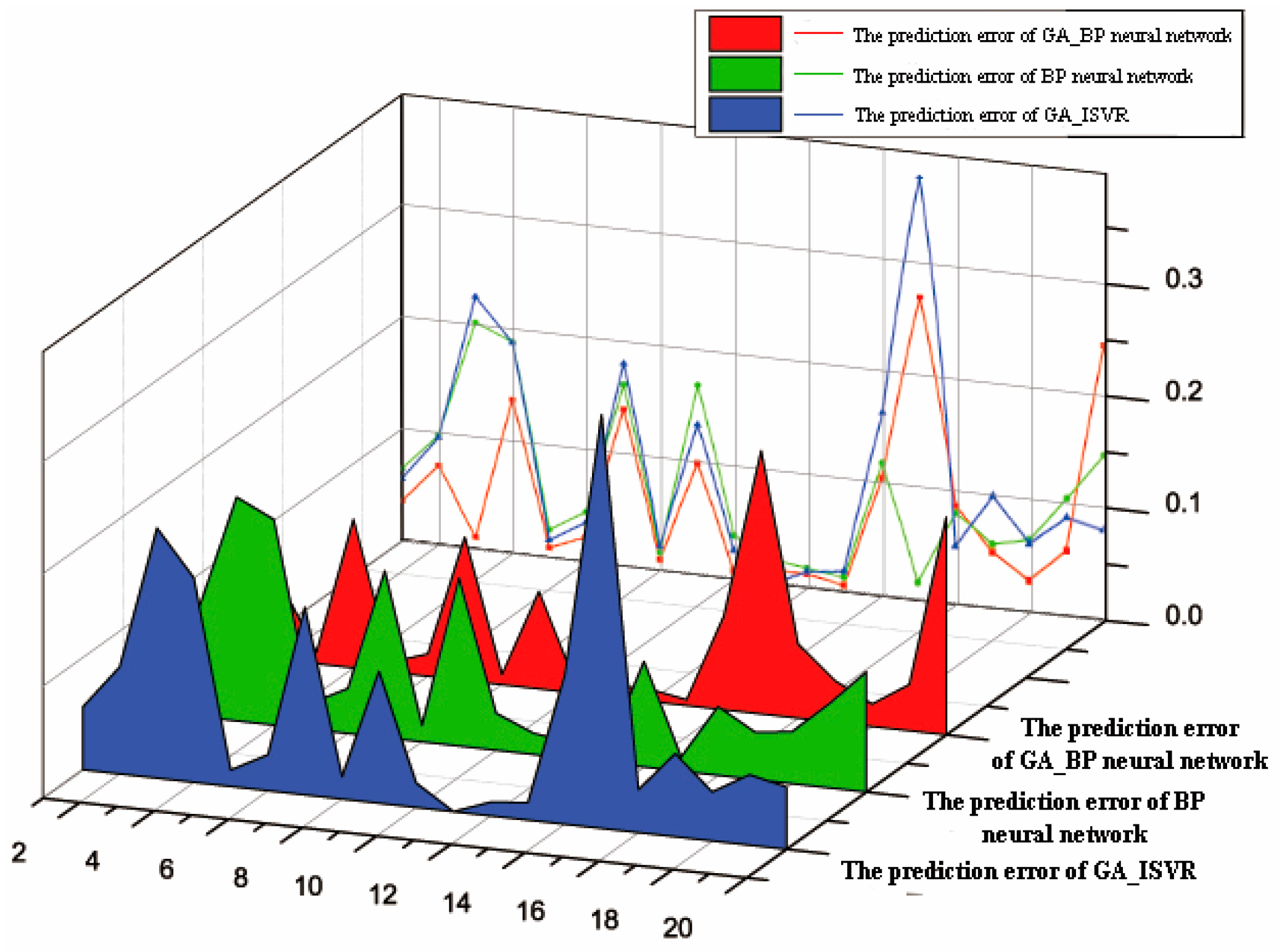
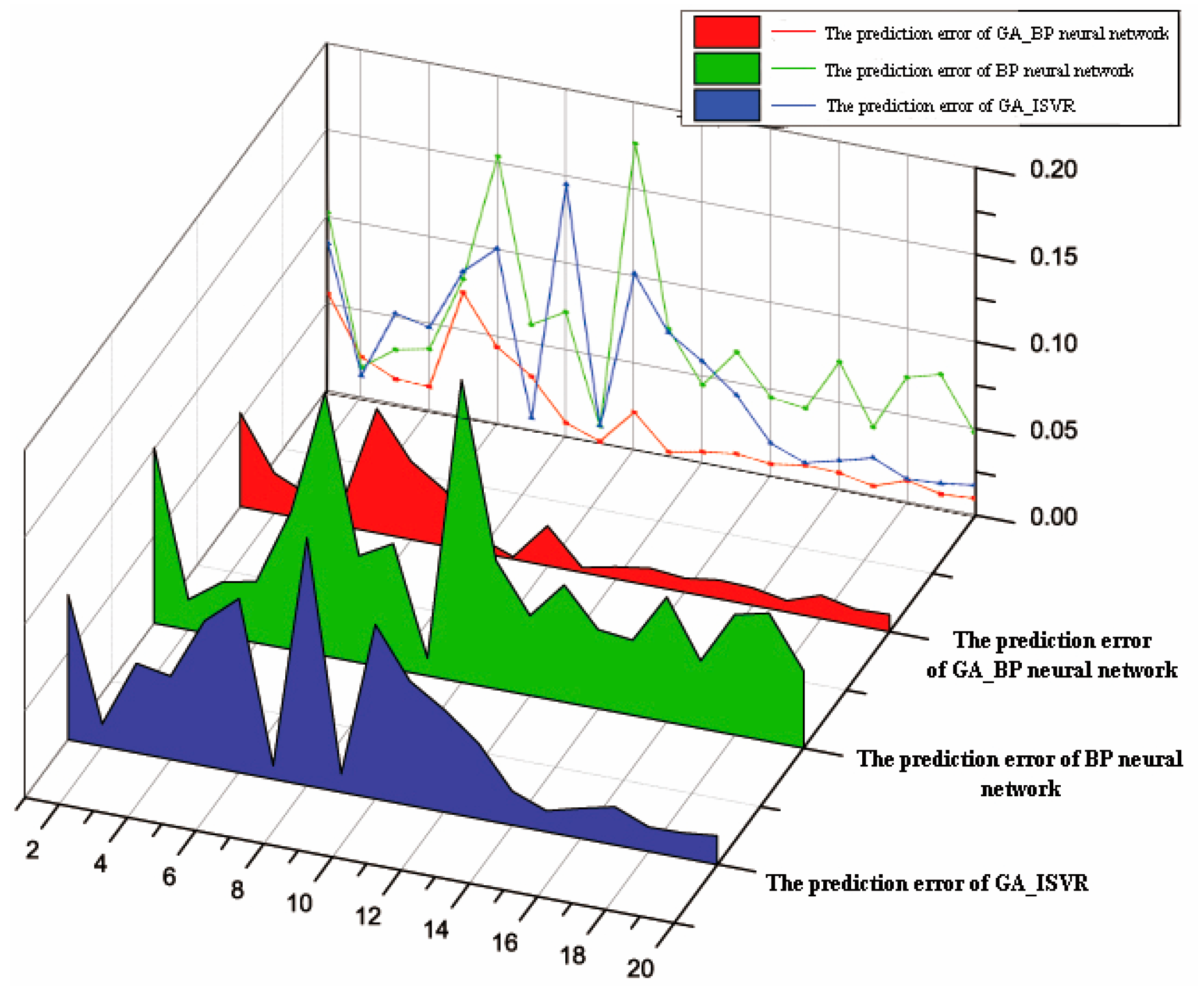
The combination of genetic algorithm and the BP neural network can improve the generalization degree and calculation accuracy of the prediction model, so as to solve the problem of insufficient accuracy caused by insufficient data quantity. Based on this, in this work, a new algorithm based on the GA_BP neural network is proposed, which is applied to the prediction and optimization of the tunnel SWB parameters. By training the input data (geological conditions and SWB parameters) and output data (overbreak/underbreak), the algorithm model builds the nonlinear relationship and realizes the prediction of the SWB effect. Moreover, based on the control of the prediction, the optimization of the design parameters of the SWB is realized.

In addition, through the analysis of the optimization of tunnel SWB parameters, it is believed that the “E_b (auxiliary hole pitch)” has the greatest impact on overbreak and underbreak. Therefore, this index should be given priority when determining parameters.

The application results demonstrate that the algorithm model is effective and feasible to predict and optimize the parameters of SWB, and the results can meet the requirements of practical engineering.

References

1. Wang, S.; Tang, Y.; Li, X.; Du, K. Analyses and Predictions of Rock Cuttabilities under Different Confining Stresses and Rock Properties Based on Rock Indentation Tests by Conical Pick. Trans. Nonferrous Met. Soc. China 2021, 31, 1766–1783. [Google Scholar] [CrossRef]
2. Wang, S.; Li, X.; Yao, J.; Gong, F.; Li, X.; Du, K.; Tao, M.; Huang, L.; Du, S. Experimental Investigation of Rock Breakage by a Conical Pick and Its Application to Non-Explosive Mechanized Mining in Deep Hard Rock. Int. J. Rock Mech. Min. Sci. 2019, 122, 104063. [Google Scholar] [CrossRef]
3. Mandal, S.K.; Singh, M.M.; Dasgupta, S. Theoretical Concept to Understand Plan and Design Smooth Blasting Pattern. Geotech. Geol. Eng. 2008, 26, 399–416. [Google Scholar] [CrossRef]
4. Mahtab, M.A.; Rossler, K.; Kalamaras, G.S.; Grasso, P. Assessment of Geological Overbreak for Tunnel Design and Contractual Claims. Int. J. Rock Mech. Min. Sci. 1997, 34, 185.e1–185.e13. [Google Scholar] [CrossRef]
5. Khandelwal, M.; Monjezi, M. Prediction of Backbreak in Open-Pit Blasting Operations Using the Machine Learning Method. Rock Mech Rock Eng. 2013, 46, 389–396. [Google Scholar] [CrossRef]
6. Jang, H.; Topal, E. Optimizing Overbreak Prediction Based on Geological Parameters Comparing Multiple Regression Analysis and Artificial Neural Network. Tunn. Undergr. Space Technol. 2013, 38, 161–169. [Google Scholar] [CrossRef]
7. Hamdi, E.; Romdhane, N.B.; Le Cléac’h, J.M. A Tensile Damage Model for Rocks: Application to Blast Induced Damage Assessment. Comput. Geotech. 2011, 38, 133–141. [Google Scholar] [CrossRef]
8. García Bastante, F.; Alejano, L.; González-Cao, J. Predicting the Extent of Blast-Induced Damage in Rock Masses. Int. J. Rock Mech. Min. Sci. 2012, 56, 44–53. [Google Scholar] [CrossRef]
9. Xia, X.; Li, H.B.; Li, J.C.; Liu, B.; Yu, C. A Case Study on Rock Damage Prediction and Control Method for Underground Tunnels Subjected to Adjacent Excavation Blasting. Tunn. Undergr. Space Technol. 2013, 35, 1–7. [Google Scholar] [CrossRef]
10. Hu, Y.; Lu, W.; Chen, M.; Yan, P.; Yang, J. Comparison of Blast-Induced Damage Between Presplit and Smooth Blasting of High Rock Slope. Rock Mech Rock Eng. 2014, 47, 1307–1320. [Google Scholar] [CrossRef]
11. Yan, P.; Lu, W.; Chen, M.; Hu, Y.; Zhou, C.; Wu, X. Contributions of In-Situ Stress Transient Redistribution to Blasting Excavation Damage Zone of Deep Tunnels. Rock Mech Rock Eng. 2015, 48, 715–726. [Google Scholar] [CrossRef]
12. Wang, S.; Sun, L.; Li, X.; Wang, S.; Du, K.; Li, X.; Feng, F. Experimental Investigation of Cuttability Improvement for Hard Rock Fragmentation Using Conical Cutter. Int. J. Geomech. 2021, 21, 06020039. [Google Scholar] [CrossRef]
13. Ryu, C.-H.; Sunwoo, C.; Lee, S.-D.; Choi, H.-M. Suggestions of Rock Classification Methods for Blast Design and Application to Tunnel Blasting. Tunn. Undergr. Space Technol. 2006, 21, 401–402. [Google Scholar] [CrossRef]
14. Yilmaz, O.; Unlu, T. An Application of the Modified Holmberg–Persson Approach for Tunnel Blasting Design. Tunn. Undergr. Space Technol. 2014, 43, 113–122. [Google Scholar] [CrossRef]
15. Monjezi, M.; Dehghani, H. Evaluation of Effect of Blasting Pattern Parameters on Back Break Using Neural Networks. Int. J. Rock Mech. Min. Sci. 2008, 45, 1446–1453. [Google Scholar] [CrossRef]
16. Wang, S.; Tang, Y.; Wang, S. Influence of Brittleness and Confining Stress on Rock Cuttability Based on Rock Indentation Tests. J. Cent. South Univ. 2021, 28, 2786–2800. [Google Scholar] [CrossRef]
17. Dai, B.; Chen, Y.; Zhao, G.; Liang, W.; Wu, H. A Numerical Study on the Crack Development Behavior of Rock-Like Material Containing Two Intersecting Flaws. Mathematics 2019, 7, 1223. [Google Scholar] [CrossRef] [Green Version]
18. Smola, A.J.; Schölkopf, B. A Tutorial on Support Vector Regression. Stat. Comput. 2004, 14, 199–222. [Google Scholar] [CrossRef] [Green Version]
19. Teymen, A.; Mengüç, E.C. Comparative Evaluation of Different Statistical Tools for the Prediction of Uniaxial Compressive Strength of Rocks. Int. J. Min. Sci. Technol. 2020, 30, 785–797. [Google Scholar] [CrossRef]
20. Hasanipanah, M.; Noorian-Bidgoli, M.; Jahed Armaghani, D.; Khamesi, H. Feasibility of PSO-ANN Model for Predicting Surface Settlement Caused by Tunneling. Eng. Comput. 2016, 32, 705–715. [Google Scholar] [CrossRef]
21. Tawadrous, A.S.; Katsabanis, P.D. Prediction of Surface Crown Pillar Stability Using Artificial Neural Networks. Int. J. Numer. Anal. Methods Geomech. 2007, 31, 917–931. [Google Scholar] [CrossRef]
22. Zhou, J.; Qiu, Y.; Armaghani, D.J.; Zhang, W.; Li, C.; Zhu, S.; Tarinejad, R. Predicting TBM Penetration Rate in Hard Rock Condition: A Comparative Study among Six XGB-Based Metaheuristic Techniques. Geosci. Front. 2021, 12, 101091. [Google Scholar] [CrossRef]
23. Dai, B.; Shan, Q.; Chen, Y.; Luo, X. Mechanical and Energy Dissipation Characteristics of Granite under Cyclic Impact Loading. J. Cent. South Univ. 2022, 29, 116–128. [Google Scholar] [CrossRef]
24. Li, Q.; Xu, Z.; Shen, X.; Zhong, J. Predicting Business Risks of Commercial Banks Based on BP-GA Optimized Model. Comput. Econ. 2021. [Google Scholar] [CrossRef]
25. Zhu, C.; Zhang, J.; Liu, Y.; Ma, D.; Li, M.; Xiang, B. Comparison of GA-BP and PSO-BP Neural Network Models with Initial BP Model for Rainfall-Induced Landslides Risk Assessment in Regional Scale: A Case Study in Sichuan, China. Nat. Hazards 2020, 100, 173–204. [Google Scholar] [CrossRef]
26. Wang, W.; Tang, R.; Li, C.; Liu, P.; Luo, L. A BP Neural Network Model Optimized by Mind Evolutionary Algorithm for Predicting the Ocean Wave Heights. Ocean Eng. 2018, 162, 98–107. [Google Scholar] [CrossRef]
27. Li, B.; Ge, W.; Li, Q.; Li, Y.; Tan, C. Gearshift Sensorless Control for Direct-Drive-Type AMT Based on Improved GA-BP Neural Network Algorithm. Math. Probl. Eng. 2020, 2020, e6456410. [Google Scholar] [CrossRef]
28. Goldberg, D.E. Genetic Algorithms in Search, Optimization and Machine Learning; Addison-Wesley: Boston, MA, USA, 1989. [Google Scholar]
29. Pineda, F.J. Generalization of Back-Propagation to recurrent neural networks. Phys. Rev. Lett. 1987, 59, 2229–2232. [Google Scholar] [CrossRef] [PubMed]
30. Mohamadnejad, M.; Gholami, R.; Ataei, M. Comparison of Intelligence Science Techniques and Empirical Methods for Prediction of Blasting Vibrations. Tunn. Undergr. Space Technol. 2012, 28, 238–244. [Google Scholar] [CrossRef]
31. Li, J.C.; Li, H.B.; Ma, G.W.; Zhou, Y.X. Assessment of Underground Tunnel Stability to Adjacent Tunnel Explosion. Tunn. Undergr. Space Technol. 2013, 35, 227–234. [Google Scholar] [CrossRef]
32. Cheng, P.; Chen, D.; Wang, J. Clustering of the Body Shape of the Adult Male by Using Principal Component Analysis and Genetic Algorithm–BP Neural Network. Soft Comput. 2020, 24, 13219–13237. [Google Scholar] [CrossRef]
33. Zheng, D.; Qian, Z.; Liu, Y.; Liu, C. Prediction and Sensitivity Analysis of Long-Term Skid Resistance of Epoxy Asphalt Mixture Based on GA-BP Neural Network. Constr. Build. Mater. 2018, 158, 614–623. [Google Scholar] [CrossRef]
34. Kavousi-Fard, A.; Khosravi, A.; Nahavandi, S. A New Fuzzy-Based Combined Prediction Interval for Wind Power Forecasting. IEEE Trans. Power Syst. 2016, 31, 18–26. [Google Scholar] [CrossRef]
35. Barzani, M.M.; Zalnezhad, E.; Sarhan, A.A.; Farahany, S.; Ramesh, S. Fuzzy logic based model for predicting surface roughness of machined Al–Si–Cu–Fe die casting alloy using different additives-turning. Measurement 2015, 61, 150–161. [Google Scholar] [CrossRef]
36. Cacciola, M.; Pellicanò, D.; Megali, G.; Lay-Ekuakille, A.; Versaci, M.; Morabito, F.C. Aspects about air pollution prediction on urban environment. In Proceedings of the 4th IMEKO TC19 Symposium on Environmental Instrumentation and Measurements, Protection Environment, Climate Changes and Pollution Control, Lecce, Italy, 3–4 June 2013; pp. 15–20. [Google Scholar]
Figure 1. The algorithm structure of GA-BP neural network.
Mathematics 10 01271 g001
Figure 2. Schematic diagram of the calculation model for parameter optimization.
Mathematics 10 01271 g002
Figure 3. SWB design parameters.
Mathematics 10 01271 g003
Figure 4. Schematic diagram for the calculation of average overbreak and underbreak.
Mathematics 10 01271 g004
Figure 5. Relationship between sample convergence speed and the number of hidden layer nodes.
Mathematics 10 01271 g005
Figure 6. Relationship between prediction error rate and number of hidden layer nodes.
Mathematics 10 01271 g006
Figure 7. Schematic diagram of GA_BP neural network topology.
Mathematics 10 01271 g007
Figure 8. Schematic diagram of the tunneling construction scheme.
Mathematics 10 01271 g008
Figure 9. Schematic diagram of the tunneling overview.
Mathematics 10 01271 g009
Figure 10. Tunneling sources of other SWB data.
Mathematics 10 01271 g010
Figure 11. GA optimized fitness curves.
Mathematics 10 01271 g011
Figure 12. Overall error of training samples in GA_BP neural network.
Mathematics 10 01271 g012
Figure 13. Schematic diagram of practical SWB construction.
Mathematics 10 01271 g013
Figure 14. Schematic diagram of practical SWB effect.
Mathematics 10 01271 g014
Figure 15. Schematic diagram of comparison between overbreak errors.
Mathematics 10 01271 g015
Figure 16. Schematic diagram of comparison between underbreak errors.
Mathematics 10 01271 g016