On the Wavelet Collocation Method for Solving Fractional Fredholm Integro-Differential Equations

Abstract

An efficient algorithm is proposed to find an approximate solution via the wavelet collocation method for the fractional Fredholm integro-differential equations (FFIDEs). To do this, we reduce the desired equation to an equivalent linear or nonlinear weakly singular Volterra–Fredholm integral equation. In order to solve this integral equation, after a brief introduction of Müntz–Legendre wavelets, and representing the fractional integral operator as a matrix, we apply the wavelet collocation method to obtain a system of nonlinear or linear algebraic equations. An a posteriori error estimate for the method is investigated. The numerical results confirm our theoretical analysis, and comparing the method with existing ones demonstrates its ability and accuracy.

1. Introduction

In this study, we propose an efficient scheme for solving the fractional Fredholm integro-differential equations (FFIDEs) of order $\alpha$ ($\alpha \in {\mathbb{R}}^{+}$) on the finite interval $[0,1]$

$${}^C{\mathcal{D}}_0^{\alpha }y\left(x\right)=c_{1}f(x,y\left(x\right))+c_2{\int }_0^{1}k(x,t)g\left(y\left(t\right)\right)dt,x\in [0,1],$$

(1)

with the Caputo fractional derivative ${}^C{\mathcal{D}}_0^{\alpha }$ and initial conditions

$$y^{\nu }\left(0\right)=y_{\nu },\nu =0,\dots ,n-1,$$

(2)

in which $c_1$, $c_2$ are constants, $\left[\alpha \right]+1:=n\in \mathbb{N}$, for $\alpha \notin \mathbb{N}$ and $n=\alpha$ for $\alpha \in \mathbb{N}$. Here, the function f is assumed to be a sufficiently smooth linear or nonlinear function on $\Omega \times \mathbb{R}$ with $\Omega :=[0,1]$, k is a continuous function on ${\mathsf{\Omega }}^2:=\mathsf{\Omega }\times \mathsf{\Omega }$, and the linear or nonlinear function g is assumed to be continuous and satisfies the Lipschitz condition

$$\left|g\right(y)-g(v\left)\right|\le \rho |y-v|,$$

(3)

where $\rho >0$ is the Lipschitz constant.

These types of equations have a very valuable role in modeling some physical phenomena, such as glass-forming process [1], epidemic processes [2], and viscoelasticity [3]. There exist several papers that offer analytical methods for solving such equations. However, when the problem is complicated, the existing analytical methods no longer work and we cannot find the exact solution. Therefore, numerical methods are often suggested to solve this problem. In [4], the Spline collocation method is applied to solve the problem. Momani et al. [5,6] used the Adomian decomposition method for solving the fourth-order and systems of FFIDEs. To solve a special type of these equations, i.e.,

$${}^C{\mathcal{D}}_0^{\alpha }y\left(x\right)-\lambda {\int }_0^{1}k(x,t){\left[y\left(t\right)\right]}^{\upsilon }dt=f\left(x\right),\upsilon >1,$$

(4)

with the initial conditions

$$y^{\left(i\right)}\left(0\right)={\delta }_i,i=0,\dots ,n-1,n-1<\alpha \le n,$$

Zhu et al. [7] proposed the Galerkin method based on the Chebyshev wavelet. After introducing the Chebyshev wavelet and the operational matrix of the Riemann–Liouville fractional integral for this basis, they used the Galerkin method to reduce (4) to a system of algebraic equations. The fractional differential transform scheme is used to solve the equation [8]. Saeedi et al. [9] used the same procedure based on CAS wavelets. Shahmorad et al. [10] proposed the Tau–like numerical algorithm to solve the delay fractional integro-differential equation. To read more about the methods provided, please refer to [11,12].

Recently, the Müntz–Legendre wavelets have been applied to find the numerical solution of some equations, such as fractional pantograph differential equations [13], fractional optimal control problems [14], fractional differential equations [15] and multi-order fractional differential equations [16].

The outline of this article is as follows: In Section 2, we provide an introduction to fractional calculation and introduce the Müntz–Legendre wavelets. Section 3 is dedicated to the application of the wavelet collocation method for solving FFIDEs. In this section, an a posteriori error estimate is also surveyed. In Section 4, some numerical implementations are performed to demonstrate the accuracy and efficiency of the method.

2. Preliminaries

We begin this section with a brief introduction to fractional calculus and the Müntz–Legendre wavelets (ML wavelets).

2.1. Fractional Calculation

Definition 1.

Let $\alpha \in {\mathbb{R}}^{+}$, we specify the Riemann–Liouville (RL) fractional integral operator ${\mathcal{I}}_a^{\alpha }$ via

$${\mathcal{I}}_a^{\alpha }\left(f\right)\left(x\right):=\frac{1}{\Gamma \left(\alpha \right)}{\int }_a^x{(x-\zeta )}^{\alpha -1}f\left(\zeta \right)d\zeta ,x\in [a,b],f\in L_1[a,b],$$

(5)

in which $\mathsf{\Gamma }\left(\alpha \right)$ is the Gamma function.

With this definition, it is easy to verify that

$${\mathcal{I}}_a^{\alpha }\left(x^{\beta }\right)=\frac{\mathsf{\Gamma }(\beta +1)}{\mathsf{\Gamma }(\beta +\alpha +1)}{x}^{\beta +\alpha }.$$

(6)

Lemma 1

(cf. Lemma 2.1 (a), [17]). Given $1\le p\le \infty$, the operator ${\mathcal{I}}_a^{\alpha }$ is bounded in $L^p\left([a,b]\right)$, i.e.,

$$\parallel {\mathcal{I}}_a^{\alpha }{\left(f\right)\parallel }_p\le \frac{{(b-a)}^{\alpha }}{\mathsf{\Gamma }(\alpha +1)}{\parallel f\parallel }_p.$$

(7)

Definition 2.

The Riemann–-Liouville operator of fractional derivative is defined by

$${}^R{\mathcal{D}}_a^{\alpha }\left(f\right)\left(x\right):={\mathcal{D}}^n{\mathcal{I}}_a^{n-\alpha }\left(f\right)\left(x\right)=\frac{1}{\mathsf{\Gamma }(n-\alpha )}{\mathcal{D}}^n{\int }_a^x{(x-t)}^{n-\alpha -1}f\left(t\right)dt,$$

(8)

where $\alpha \in {\mathbb{R}}^{+}$, $\left[\alpha \right]+1:=n\in \mathbb{N}$ and ${\mathcal{D}}^n:=\frac{d^n}{dx}$.

There exists another fractional derivative operator that can replace the Riemann–Liouville fractional derivative.

Definition 3.

The Caputo fractional derivative is determined by [17].

$$\begin{array}{cc}\hfill {}^c{\mathcal{D}}_a^{\alpha }\left(f\right)\left(x\right):& =\frac{1}{\mathsf{\Gamma }(n-\alpha )}{\int }_a^x\frac{f^{\left(n\right)}\left(\zeta \right)d\zeta }{{(x-\zeta )}^{\alpha -n+1}}=:{\mathcal{I}}_a^{n-\alpha }{\mathcal{D}}^n\left(f\right)\left(x\right),\hfill \end{array}$$

(9)

in which $\alpha \in {\mathbb{R}}^{+}$ and $\left[\alpha \right]+1:=n\in \mathbb{N}$.

Lemma 2

(cf. Corollary 2.3 (a), [17]). It can be proved that the Caputo fractional derivative operator ${}^c{\mathcal{D}}_a^{\alpha }$ is bounded via

$$\parallel {}^c{\mathcal{D}}_a^{\alpha }{\left(f\right)\parallel }_C\le \frac{1}{\mathsf{\Gamma }(n-\alpha )(n-\alpha +1)}{\parallel f\parallel }_{C^n},$$

(10)

where $\alpha \in {\mathbb{R}}^{+}$, $\alpha \notin {\mathbb{N}}_0$ and $n=-[-\alpha ]$.

2.2. Müntz–Legendre Wavelets

For $J\in {\mathbb{N}}_0$ and $r\in \mathbb{N}$, let $\mathcal{R}:=\{0,1,\dots ,r-1\}$ and $\mathcal{B}:=\{0,1,\dots ,2^J-1\}$. Then assume that the sub-space $A_J\in L^2\left(\mathsf{\Lambda }\right)$ is spanned by

$$A_J=span\{{\varphi }_{J,b}^n:n\in \mathcal{R},b\in \mathcal{B}\},$$

in which ${\varphi }_{J,b}^n$ is the scaled and translated version of ${\varphi }^n$, and $\mathsf{\Lambda }$ is a bounded interval or $\mathsf{\Lambda }:=\mathbb{R}$. Furthermore, the parameters J and r are called the refinement level and multiplicity, respectively.

At the sequel, we give a brief introduction to the ML wavelets that, in addition to spanned $V_J$, they also satisfy certain circumstances [18] (namely, multiresolution analysis (MRA)).

Motivated by [19], an increasing sequence $\mathcal{L}=\{0={\lambda }_0<{\lambda }_1<\dots \}$ guarantees that the vector space

$$P\left(\mathcal{L}\right):=\bigcup _{n=0}^{\infty }{P}_n\left(\mathcal{L}\right)=span\{x^{{\lambda }_n},n=0,1,\dots \},x\in (0,1),$$

spanned by ${\left\{x^{{\lambda }_n}\right\}}_{n=0}^{\infty }$ and is a dense subset of $C[0,1]$. Here $P_n\left(\mathcal{L}\right):=span\{x^{{\lambda }_0},x^{{\lambda }_1},\dots ,x^{{\lambda }_n}\}$ for each n. The Russian mathematician S. N. Bernstein specifically proved that the sufficient and necessary conditions to have $\overline{P\left(\mathcal{L}\right)}=C[0,1]$ are

$$\sum _{{\lambda }_k>0}\frac{1+log{\lambda }_k}{{\lambda }_k}=\infty ,$$

and

$$\underset{k\to \infty }{lim}\frac{{\lambda }_k}{klogk}=0,$$

respectively. He also conjectured that the necessary and sufficient condition to have $\mathcal{L}=\{0={\lambda }_0<{\lambda }_1<\dots \}$ is

$$\sum _{k=1}^{\infty }\frac{1}{{\lambda }_k}=\infty .$$

Two years later, Müntz proved this conjecture [20]. It can be shown that the same result can be held for $L^2(0,1)$ [21]. It is worth noting that the functions ${\left\{x^{{\lambda }_n}\right\}}_{n=0}^{\infty }$ are not suitable as basis functions. Thus, in the sequel, the Müntz–Legendre functions will be introduced such that they are easy to evaluate and are orthogonal.

Motivated by [21,22], the ML polynomials are determined by

$$L_n(x;\mathcal{L}):=\frac{1}{2\pi i}{\int }_A\prod _{k=1}^{n-1}\frac{s+{\lambda }_k+1}{s-{\lambda }_k}\frac{x^s}{s-{\lambda }_n}ds,$$

(11)

where A is a simple contour which is circumambient to all zeros of the denominator in the integrand. The aforementioned polynomials can be shown via

$$L_n(x;\mathcal{L})=\sum _{l=0}^n{l}_{l,n}{x}^{{\lambda }_l},x\in [0,1],$$

(12)

where the coefficient $l_{l,n}$ is obtained by

$$l_{l,n}:=\frac{{\prod }_{i=0}^{n-1}({\lambda }_l+{\lambda }_i+1)}{{\prod }_{i=0,i\ne l}^n({\lambda }_l-{\lambda }_i)}.$$

(13)

in which ${\lambda }_l:=\{l\mu :\mu \in \mathbb{R},l=0,\dots n\}$. It can easily be shown that the ML polynomials are orthogonal [21,22].

For simplicity, assume that $L_n\left(x\right):=L_n(x;\mathcal{L})$ from now on. According to the definition of $L_n\left(x\right)$, the ML wavelets [16] can be obtained via

$${\varphi }_{J,b}^n=\left\{\begin{array}{cc}{2}^{J/2}\sqrt{2{\lambda }_n+1}{L}_n(2^{J}x-b),\hfill & \frac{b}{2^J}\le x\le \frac{b+1}{2^J},\hfill \\ 0,\hfill & \mathrm{otherwise}.\hfill \end{array}\right.$$

(14)

Motivated by ML wavelets, we introduce a projection operator ${\mathcal{P}}_J$ that maps any function $y\in L^2\left([0,1]\right)$ onto $A_J$ as follows.

$$y\left(x\right)\approx {\mathcal{P}}_J\left(y\right)\left(x\right)=\sum _{b=0}^{2^J-1}\sum _{n=0}^{r-1}{y}_{b,n}{\varphi }_{J,b}^n\left(x\right)=U^T\mathsf{\Phi }\left(x\right)\in A_J,$$

(15)

where $\mathsf{\Phi }\left(x\right)$ is a $N=2^{J}r$ dimensional vector function whose $(br+n+1)$-th element is ${\varphi }_{J,b}^n\left(x\right)$. To evaluate the element of vector U, we have

$$y_{b,n}=\langle y,{\varphi }_{J,b}^n\rangle ={\int }_0^{1}y\left(x\right){\varphi }_{J,b}^n\left(x\right)dx.$$

(16)

The aforementioned expansion (15) can be bounded as follows [13].

Lemma 3

([13]). If $y\in H^m\left([0,1]\right)$ for $r>m$, then

$$\parallel y-{\mathcal{P}}_J{\left(y\right)\parallel }_{L_2\left([0,1]\right)}\le c{(r-1)}^{-m}{\left(2^{J-1}\right)}^{-m}{\parallel y^{\left(m\right)}\parallel }_{L_2\left([0,1]\right)},$$

(17)

and when $s\ge 1$, we get

$$\parallel y-{\mathcal{P}}_J{\left(y\right)\parallel }_{H^s\left([0,1]\right)}\le c{\left(2^{J-1}\right)}^{s-m}{(r-1)}^{2s-\frac{1}{2}-m}{\parallel y^{\left(m\right)}\parallel }_{L_2\left([0,1]\right)},$$

(18)

in which $H^m\left([0,1]\right)$ is the Sobolev space and the related norm is determined by

$${\parallel y\parallel }_{H^m\left([0,1]\right)}={\left(\sum _{j=0}^m{\parallel y^{\left(j\right)}\parallel }_{L_2\left([0,1]\right)}^2\right)}^{1/2}.$$

2.3. Representation of Fractional Integral Operator in ML Wavelets

The fractional integration of the vector function ${\mathsf{\Phi }}_J\left(x\right)$ can be expressed by

$${\mathcal{P}}_J\left({\mathcal{I}}_0^{\alpha }\right)\left(\mathsf{\Phi }\left(x\right)\right)\approx I_{\alpha }\mathsf{\Phi }\left(x\right),x\in (0,1),$$

(19)

where $I_{\alpha }$ is called the Riemann–Liouville fractional operational matrix.

In order to find the elements of $I_{\alpha }$ for ML wavelets, we need to introduce the piecewise fractional-order Taylor functions, i.e.,

$${\psi }_{J,b}^n=\left\{\begin{array}{cc}{t}^{{\lambda }_n},\hfill & \frac{b}{2^J}\le x\le \frac{b+1}{2^J},\hfill \\ 0,\hfill & otherwise,\hfill \end{array}\right.b\in \mathcal{B},n\in \mathcal{R},J\in {\mathbb{Z}}^{+}\cup \left\{0\right\}.$$

(20)

Using the vector function $\Psi \left(x\right)$ whose elements are ${\psi }_{J,b}^n$, the vector function $\mathsf{\Phi }\left(x\right)$ (ML wavelets) can be represented by

$$\mathsf{\Phi }\left(x\right)=T^{-1}\Psi \left(x\right),$$

(21)

where the transformation matrix T is the square matrix of dimension $N\times N$ with elements

$$T_{i,j}=\langle {\mathsf{\Phi }}_i\left(x\right),{\Psi }_j\left(x\right)\rangle ={\int }_0^1{\mathsf{\Phi }}_i\left(x\right){\Psi }_j\left(x\right)dx,i,j=1,\dots ,N.$$

(22)

It can be shown that

$$\Psi \left(x\right)={\left[V,\dots ,V\right]}^T,$$

(23)

in which V is assumed to be a r-dimension vector whose i-th element is $x^{{\lambda }_i}$. From (6), one can calculate the fractional integral of the i-th element $\Psi \left(x\right)$, i.e.,

$${\mathcal{I}}_0^{\alpha }\left({\Psi }_i\right)\left(x\right)=\frac{\mathsf{\Gamma }({\lambda }_i+1)}{\mathsf{\Gamma }({\lambda }_i+\alpha +1)}{x}^{{\lambda }_i+\alpha }.$$

(24)

Therefore, there exists a matrix $I_{\Psi ,\alpha }\left(x\right)$ such that

$${\mathcal{I}}_0^{\alpha }(\Psi )\left(x\right)=I_{\Psi ,\alpha }\left(x\right)\Psi \left(x\right).$$

(25)

It can easily be demonstrated that

$$I_{\Psi ,\alpha }\left(x\right)=diag\left[P_{\alpha }\left(x\right),\dots ,P_{\alpha }\left(x\right)\right],$$

in which $P_{\alpha }\left(x\right):=x^{\alpha }Q$$({\mathcal{I}}_0^{\alpha }\left(V\right)\left(x\right)=P_{\alpha }\left(x\right)V\left(x\right))$, and Q is a diagonal matrix

$${\left(Q\right)}_{i,i}=\left(\mathsf{\Gamma }({\lambda }_i+1)\right){\left(\mathsf{\Gamma }({\lambda }_i+\alpha +1)\right)}^{-1}.$$

Now, we can obtain the fractional integral operational matrix for the ML wavelets

$$\begin{array}{cc}\hfill {\mathcal{P}}_J\left({\mathcal{I}}_0^{\alpha }\right)\left(\mathsf{\Phi }\left(x\right)\right)& ={\mathcal{P}}_J\left({\mathcal{I}}_0^{\alpha }\right)(T^{-1}\Psi \left(x\right))\hfill \\ \hfill & =T^{-1}{I}_{\Psi ,\alpha }\left(x\right)\Psi \left(x\right)\hfill \\ \hfill & =T^{-1}{I}_{\Psi ,\alpha }\left(x\right)T\mathsf{\Phi }\left(x\right).\hfill \end{array}$$

Thus we obtain

$$I_{\alpha }\left(x\right):=T^{-1}{I}_{\Psi ,\alpha }\left(x\right)T.$$

(26)

3. Wavelet Collocation Method

In the present section, we utilize the collocation method based on ML wavelets to obtain an approximate solution of the fractional Fredholm integro-differential Equation (1). In the operator form, Equation (1) may be written as

$$({}^C{\mathcal{D}}_0^{\alpha }-c_2\mathcal{K})y=c_{1}f,$$

(27)

in which the operator $\mathcal{K}$ is denoted by

$$\mathcal{K}\left(y\right)\left(x\right):={\int }_0^{1}k(x,t)g\left(y\left(t\right)\right)dt.$$

(28)

If y is a sufficiently smooth function on $[0,1]$, it can be proved that Equation (1) has a unique solution $y\left(x\right)$ on $[0,1]$.

Lemma 4.

Given $\alpha \in {\mathbb{R}}^{+}$, let $n=-[-\alpha ]$. Assume that f, k, and u are continuous functions. Then $y\left(x\right)$ is the solution of (1) if, and only if, $y\left(x\right)$ satisfies the integral equation

$$y\left(x\right)=\sum _{j=0}^{n-1}\frac{y^{\left(i\right)}\left(0\right)}{j!}{x}^j+c_1{\mathcal{I}}_0^{\alpha }\left(f\right)(x,y\left(x\right))+c_2{\mathcal{I}}_0^{\alpha }\mathcal{K}\left(y\right)\left(x\right),$$

(29)

Proof. 

The proof is similar to the proof of Theorem 3.24 in [17]. □

To obtain the discretization of (29), the numerical solution may be approximated by the operator ${\mathcal{P}}_J$, i.e.,

$$y\left(x\right)\approx {\mathcal{P}}_J\left(y\right)\left(x\right)=U^T\mathsf{\Phi }\left(x\right):=y_J\left(x\right),$$

(30)

where U is a N-dimension vector whose elements should be found. Replacing (30) into (29), we get

$$y_J\left(x\right)=\sum _{j=0}^{n-1}\frac{y^{\left(i\right)}\left(0\right)}{j!}{x}^j+c_1{\mathcal{I}}_0^{\alpha }\left(f\right)(x,y_J\left(x\right))+c_2{\mathcal{I}}_0^{\alpha }\left(\mathcal{K}\right)\left(y_J\right)\left(x\right).$$

(31)

Now, we transfer all terms in (31) onto $A_J$ via the projection operator ${\mathcal{P}}_J$ as follows

• Let us put $p_1\left(x\right):={\sum }_{j=0}^{n-1}\frac{y^{\left(i\right)}\left(0\right)}{j!}{x}^j$, then we can write

  $$p_1\left(x\right)\approx {\mathcal{P}}_J\left(p_1\right)\left(x\right)=P_1^T\mathsf{\Phi }\left(x\right),$$

  (32)

  where the j-th element of the N dimensional vector $P_1$ is obtained by $\langle p_1,{\mathsf{\Phi }}_j\rangle$.
• After putting the approximate solution $y_J$ into $g\left(y\right(t\left)\right)$ and then approximating it and the kernel function $k(x,t)$ using operator ${\mathcal{P}}_J$, we have

  $$\begin{array}{cc}\hfill p_2\left(t\right):=g\left(y_J\left(t\right)\right)& \approx {\mathcal{P}}_J\left(g\left(y_J\left(t\right)\right)\right)=G^T\mathsf{\Phi }\left(t\right),\hfill \\ \hfill k(x,t)& \approx {\mathcal{P}}_J\left(k\right)(x,t)={\mathsf{\Phi }}^T\left(x\right)K\mathsf{\Phi }\left(t\right),\hfill \end{array}$$

  (33)

  where G is an N-dimensional vector whose j-th element is $\langle p_2,{\mathsf{\Phi }}_j\rangle$, and K is a square matrix of dimension $N\times N$ whose $(i,j)$-element is

  $$K_{i,j}={\int }_0^1{\int }_0^{1}k(x,t){\mathsf{\Phi }}_i\left(x\right){\mathsf{\Phi }}_j\left(t\right)dxdt.$$
  Replacing (33) into $\mathcal{K}\left(y_J\right)\left(x\right)$, we obtain

  $${\mathcal{P}}_J\mathcal{K}\left(y_J\right)\left(x\right)\approx G^T{K}^T\mathsf{\Phi }\left(x\right)\in A_J,$$

  (34)
  To give rise to the discretized form of ${\mathcal{I}}_0^{\alpha }\mathcal{K}\left(y_J\right)\left(x\right)$, using the operational matrix $I_{\alpha }$ and (35), we obtain

  $${\mathcal{I}}_0^{\alpha }\mathcal{K}\left(y_J\right)\left(x\right)\approx G^T{K}^T{I}_{\alpha }\left(x\right)\mathsf{\Phi }\left(x\right).$$

  (35)
• In the same way as the previous item, we can use the projection ${\mathcal{P}}_J$ for the term ${\mathcal{I}}_0^{\alpha }\left(f\right)(s,y\left(s\right))$, as

  $$\begin{array}{cc}\hfill {\mathcal{I}}_0^{\alpha }\left(f\right)(s,y_J\left(s\right))& \approx {\mathcal{I}}_0^{\alpha }\left(F^T\mathsf{\Phi }\left(x\right)\right)\hfill \\ \hfill & \approx F^T{I}_{\alpha }\left(x\right)\mathsf{\Phi }\left(x\right),\hfill \end{array}$$

  (36)

  where F is a N-dimension vector whose j-th element is $\langle f,{\mathsf{\Phi }}_j\rangle$.

Now we refer to (29) and rewrite it using (32), (35) and (36) as follows.

$$r\left(x\right):=\left(U^T-P_1^T-c_1{F}^T{I}_{\alpha }\left(x\right)-G^T{K}^T{I}_{\alpha }\left(x\right)\right)\mathsf{\Phi }\left(x\right)=0,$$

(37)

where $r\left(x\right)$ is the residual function that our goal is to reduce to zero. By choosing the collocation points $\left\{x_i\right\}\in \mathsf{\Omega }$ which satisfy $r\left(x_i\right)=0$, we obtain a system of nonlinear or linear algebraic equations. After solving this system, we can find the unknown coefficients U. Here, the collocation points are chosen so that they are the roots of the shifted Chebyshev and Legendre polynomials.

Error Analysis

Theorem 1.

Assume that $k(x,t)$ is a sufficiently smooth function on $[0,1]\times \mathbb{R}$ and the functions g and f are continuous and satisfy the Lipschitz conditions (3) and

$$\left|f\right(x,y\left(x\right))-f(x,v\left(x\right)\left)\right|\le \varrho |y-v|,$$

(38)

respectively.

If $c_1\frac{\rho M_1}{\alpha \mathsf{\Gamma }\left(\alpha \right)}+c_2\frac{\varrho }{\mathsf{\Gamma }(\alpha +1)}<1$ with $\alpha \in (0,1)$, and $M_1={max}_{x,t\in [0,1]}\left|k(x,t)\right|$, then the a posteriori error estimate can be found as,

$$\parallel y\left(x\right)-y_J\left(x\right)\parallel \le \frac{C}{1-\eta }{(r-1)}^{-m}{\left(2^{J-1}\right)}^{-m}.$$

Proof. 

Motivated by Lemma 3, we have

$$\parallel {\mathcal{I}}_0^{\alpha }\mathcal{K}\left(y_J\right)-{\mathcal{P}}_J{\mathcal{I}}_0^{\alpha }\mathcal{K}\left(y_J\right)\parallel \le c_0{(r-1)}^{-m}{\left(2^{J-1}\right)}^{-m}{M}_2,$$

(39)

where $M_2=max\left\{{\mathcal{D}}^m{\mathcal{I}}_0^{\alpha }\mathcal{K}\left(y_J\right)\right\}$, and to approximate it, we can consider two situations.

1.

if $m<n$, then we have

$${\mathcal{D}}^m{\mathcal{I}}_0^{\alpha }\mathcal{K}\left(y_J\right)={\mathcal{I}}_0^{\alpha -m}\mathcal{K}\left(y_J\right),$$

(40)

and it follows from Lemma 1 that

$$\begin{array}{cc}\hfill \parallel {\mathcal{D}}^m{\mathcal{I}}_0^{\alpha }\mathcal{K}\left(y_J\right)\parallel =\parallel {\mathcal{I}}_0^{\alpha -m}\mathcal{K}\left(y_J\right)\parallel & \le \frac{1}{\mathsf{\Gamma }(\alpha -m+1)}\parallel \mathcal{K}\left(y_J\right)\parallel \hfill \\ \hfill & \le \frac{M_1}{\mathsf{\Gamma }(\alpha -m+1)}\parallel {\int }_0^{1}g\left(y_J\left(t\right)\right)dt\parallel \hfill \\ \hfill & \le \frac{M_1}{\mathsf{\Gamma }(\alpha -m+1)}{\int }_0^1\parallel g\left(y_J\left(t\right)\right)\parallel dt\hfill \end{array}$$

(41)

Since the function g is continuous, then $\parallel {\mathcal{D}}^m{\mathcal{I}}_0^{\alpha }\mathcal{K}{y}_J\parallel$ is bounded.

2.

Let $m\ge n$. Motivated by the Lemma 2.21 [17], it is easy to write

$${\mathcal{D}}^m{\mathcal{I}}_0^{\alpha }\mathcal{K}\left(y_J\right)={}^C{\mathcal{D}}^{m-\alpha }{}^C{\mathcal{D}}^{\alpha }{\mathcal{I}}_0^{\alpha }\mathcal{K}\left(y_J\right)={}^C{\mathcal{D}}^{m-\alpha }\mathcal{K}\left(y_J\right).$$

(42)

Taking the norm from both sides of (42) and using Lemma 2, we have

$$\begin{array}{cc}\hfill \parallel {\mathcal{D}}^m{\mathcal{I}}_0^{\alpha }\mathcal{K}\left(y_J\right)\parallel & =\parallel {}^C{\mathcal{D}}^{m-\alpha }\mathcal{K}\left(y_J\right)\parallel \hfill \\ \hfill & \le \frac{1}{\mathsf{\Gamma }(m^{\prime }-m+\alpha )(m^{\prime }-m+\alpha +1)}\parallel \mathcal{K}\left(y_J\right)\parallel (m^{\prime }=[m-\alpha ]+1).\hfill \end{array}$$

(43)

As a result, we can bound this case according to the previous one.

Further, we can obtain

$$\parallel {\mathcal{I}}_0^{\alpha }\left(f\right)(x,y_J)-{\mathcal{P}}_J{\mathcal{I}}_0^{\alpha }\left(f\right)(x,y_J)\parallel \le c_3{(r-1)}^{-m}{\left(2^{J-1}\right)}^{-m}{M}_3,$$

(44)

and

$$\parallel {\mathcal{I}}_0^{\alpha }\left(p_1\right)(x,y_J)-{\mathcal{P}}_J{\mathcal{I}}_0^{\alpha }\left(p_1\right)(x,y_J)\parallel \le c_4{(r-1)}^{-m}{\left(2^{J-1}\right)}^{-m}{M}_4,$$

(45)

in which $M_3={max}_{\xi \in [0,1]}\left\{{\mathcal{D}}^m{\mathcal{I}}_0^{\alpha }f(\xi ,y_J\left(\xi \right))\right\}$, and $M_4={max}_{\xi \in [0,1]}\left\{{\mathcal{D}}^m{\mathcal{I}}_0^{\alpha }{p}_1(\xi ,y_J\left(\xi \right))\right\}$. Similar to the process used to calculate $M_2$, it can be used to approximate $M_3$ and $M_4$.

If k is a continuous function and g satisfies the Lipschitz condition (3), then we can write

$$\begin{array}{cc}\hfill \parallel {\mathcal{I}}_0^{\alpha }\mathcal{K}\left(y\right)-{\mathcal{I}}_0^{\alpha }\mathcal{K}\left(y_J\right)\parallel & =\parallel {\mathcal{I}}_0^{\alpha }\left({\int }_0^{1}k(x,t)g\left(y\left(t\right)\right)dt-{\int }_0^{1}k(x,t)g\left(y_J\left(t\right)\right)dt\right)\parallel \hfill \\ \hfill & \le \parallel {\mathcal{I}}_0^{\alpha }\left(\rho {\int }_0^{1}k(x,t)(y\left(t\right)-y_J\left(t\right))dt\right)\parallel \hfill \\ \hfill & \le \parallel {\mathcal{I}}_0^{\alpha }\left(\rho M_1{\int }_0^1(y\left(t\right)-y_J\left(t\right))dt\right)\parallel (M_1:=ma{x}_{x,t\in [0,1]}\left|k(x,t)\right|)\hfill \\ \hfill & \le \frac{\rho M_1}{\mathsf{\Gamma }\left(\alpha \right)}{\int }_0^x{(x-t)}^{\alpha -1}{\int }_0^1\parallel y-y_J\parallel dsdt\hfill \\ \hfill & \le \frac{\rho M_1}{\mathsf{\Gamma }\left(\alpha \right)}\parallel y-y_J\parallel {\int }_0^x{(x-t)}^{\alpha -1}dt\hfill \\ \hfill & \le \frac{\rho M_1}{\alpha \mathsf{\Gamma }\left(\alpha \right)}\parallel y-y_J\parallel .\hfill \end{array}$$

(46)

It is easy to find a bound for $\parallel ({\mathcal{I}}_0^{\alpha }\left(f\right)(x,y\left(x\right))-{\mathcal{I}}_0^{\alpha }\left(f\right)(x,y_J\left(x\right)))\parallel$ according to the Lemma 1, via

$$\begin{array}{cc}\hfill \parallel {\mathcal{I}}_0^{\alpha }\left(f\right)(x,y\left(x\right))-{\mathcal{I}}_0^{\alpha }\left(f\right)(x,y_J\left(x\right))& \parallel \le \varrho \parallel {\mathcal{I}}_0^{\alpha }(y-y_J)\parallel \hfill \\ \hfill & \le \frac{\varrho }{\mathsf{\Gamma }(\alpha +1)}\parallel y-y_J\parallel .\hfill \end{array}$$

(47)

Subtracting (29) from

$$y_J\left(x\right)={\mathcal{P}}_J\left(p_1\right)\left(x\right)+c_1{\mathcal{P}}_J\left({\mathcal{I}}_0^{\alpha }\right)\left(f\right)(x,y_J\left(x\right))+c_2{\mathcal{P}}_J\left({\mathcal{I}}_0^{\alpha }\right)\left(\mathcal{K}\right)\left(y_J\right)\left(x\right),$$

(48)

and taking the norm from both sides, it follows from (39), (44)–(47) that

$$\begin{array}{cc}\hfill \parallel y-y_J\parallel & \le \parallel p_1-{\mathcal{P}}_J\left(p_1\right)\parallel +c_1\parallel {\mathcal{I}}_0^{\alpha }\left(f\right)(x,y\left(x\right))-{\mathcal{I}}_0^{\alpha }\left(f\right)(x,y_J\left(x\right))\parallel \hfill \\ \hfill & +c_1\parallel {\mathcal{I}}_0^{\alpha }\left(f\right)(x,y_J\left(x\right))-c_1{\mathcal{P}}_J{\mathcal{I}}_0^{\alpha }\left(f\right)(x,y_J\left(x\right))\parallel \hfill \\ \hfill & +c_2\parallel {\mathcal{I}}_0^{\alpha }\mathcal{K}\left(y\right)\left(x\right)-{\mathcal{I}}_0^{\alpha }\mathcal{K}\left(y_J\right)\left(x\right)\parallel \hfill \\ \hfill & +c_2\parallel {\mathcal{I}}_0^{\alpha }\mathcal{K}\left(y_J\right)\left(x\right)-{\mathcal{P}}_J\left({\mathcal{I}}_0^{\alpha }\right)\mathcal{K}\left(y_J\right)\left(x\right)\parallel \hfill \\ \hfill & \le C{(r-1)}^{-m}{\left(2^{J-1}\right)}^{-m}+\eta \parallel y-y_J\parallel \hfill \end{array}$$

(49)

in which $C=c_4{M}_4+c_1{c}_3{M}_3+c_2{c}_0{M}_2$ and $\eta =c_1\frac{\varrho }{\mathsf{\Gamma }(\alpha +1)}+c_2\frac{\rho M_1}{\alpha \mathsf{\Gamma }\left(\alpha \right)}$. If $\eta <1$, then we can bound the error as follows.

$$\parallel y\left(x\right)-y_J\left(x\right)\parallel \le \frac{C}{1-\eta }{(r-1)}^{-m}{\left(2^{J-1}\right)}^{-m}.$$

(50)

□

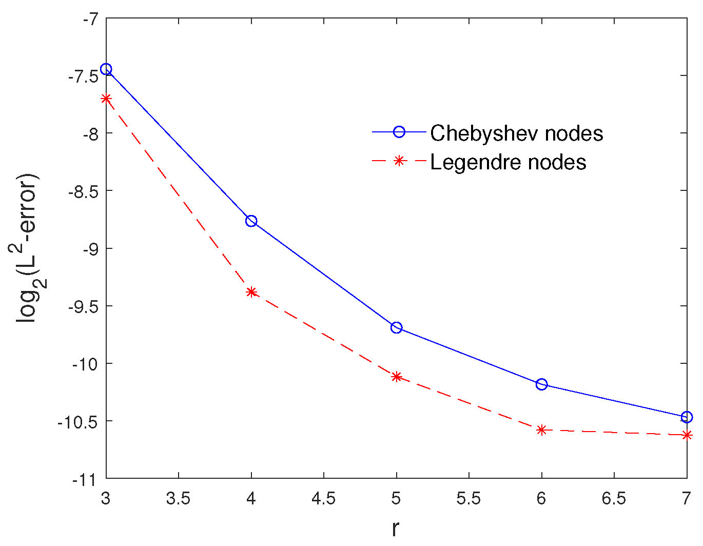
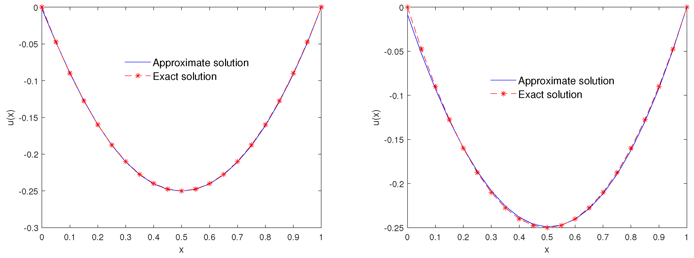
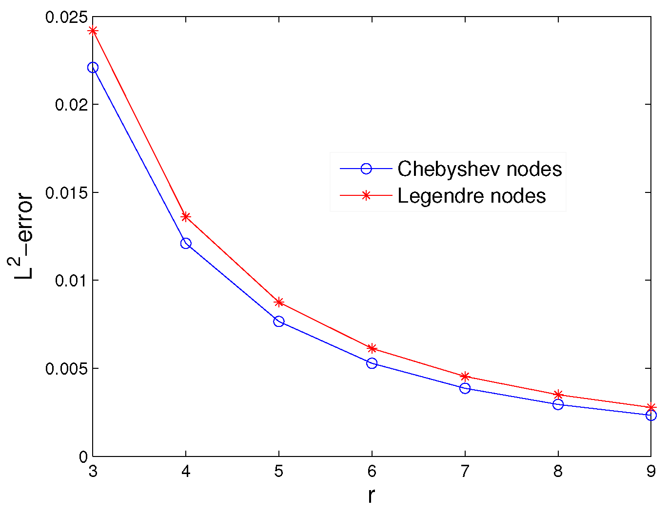
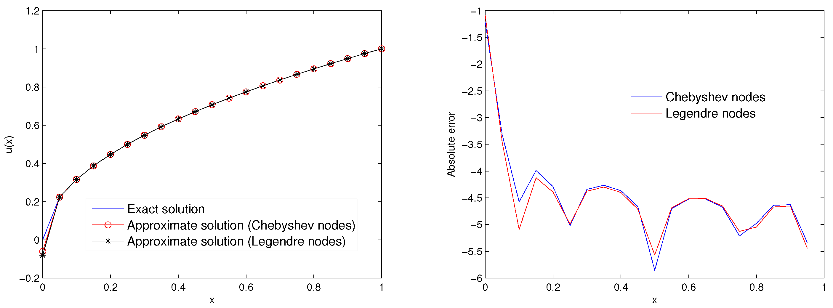
4. Numerical Experiments

All numerical computations were carried out simultaneously using Maple and Matlab software.

Example 1.

Consider the following equation [23] as the first example.

$${}^C{\mathcal{D}}_0^{5/6}u\left(x\right)+{\int }_0^{1}x{e}^t{\left(u\left(t\right)\right)}^{2}dt=\frac{3}{\mathsf{\Gamma }(1/6)}\left(2\sqrt[6]{x}-\frac{432}{91}\sqrt[6]{x^{13}}\right)-x(248e-674),$$

with initial condition $u\left(0\right)=0$. The exact solution is reported in [23] as $u\left(x\right)=x-x^3$.

Table 1. The comparison between Alpert’s multiwavelets method and the proposed method taking $\mu =5/6$ and Chebyshev nodes for Example 1.

	Proposed Method			Alpert’s Multiwavelets Method [23]
	$N=4$	$N=5$	$N=7$	$N=96$
$L^2$-error	$1.78\times {10}^{-3}$	$4.08\times {10}^{-4}$	$1.72\times {10}^{-4}$	$1.43\times {10}^{-3}$

gives a comparison between the proposed method and Alpert’s multi-wavelets method. It can be seen that our method offers better accuracy. The $L_{\infty }$-error is reported for different values of r ($N=r{2}^J$) and x in

Table 2. The $L_{\infty }$–error taking $\mu =5/6$ for Example 1.

		$\mathit{x}=0.1$	$\mathit{x}=0.3$	$\mathit{x}=0.5$	$\mathit{x}=0.7$	$\mathit{x}=0.9$
Chebyshev nodes	$N=5$	$6.62\times {10}^{-4}$	$3.41\times {10}^{-4}$	$2.17\times {10}^{-4}$	$1.98\times {10}^{-6}$	$1.89\times {10}^{-4}$
	$N=7$	$1.65\times {10}^{-5}$	$2.09\times {10}^{-6}$	$9.63\times {10}^{-6}$	$2.77\times {10}^{-5}$	$6.68\times {10}^{-5}$
Legendre nodes	$N=5$	$2.84\times {10}^{-4}$	$6.80\times {10}^{-5}$	$2.19\times {10}^{-4}$	$2.70\times {10}^{-4}$	$4.69\times {10}^{-5}$
	$N=7$	$2.95\times {10}^{-4}$	$1.07\times {10}^{-4}$	$9.61\times {10}^{-6}$	$8.85\times {10}^{-5}$	$1.48\times {10}^{-4}$

. To show the effect of the parameters μ and r in the $L^2$-error, we plot the Figure 1.

Example 2.

Consider the nonlinear FFIDEs [23]

$${}^C{\mathcal{D}}_0^{1/2}u\left(x\right)+{\int }_0^{1}xt{\left(u\left(t\right)\right)}^{4}dt=\frac{1}{\mathsf{\Gamma }(1/2)}\left(8/3x^{3/2}-2x^{1/2}\right)-\frac{x}{1260},x\in [0,1]$$

subject to the initial condition $u\left(0\right)=0$. The exact solution is $u\left(x\right)=x^2-x$ [23].

To show the effect of the parameter r in the $L^2$-error, we plot the Figure 2. A comparison between the proposed method and Alpert’s multi-wavelets method is reported in

Table 3. The $L_{\infty }$–error taking $\mu =1$ for Example 2.

		$\mathit{x}=0.1$	$\mathit{x}=0.3$	$\mathit{x}=0.5$	$\mathit{x}=0.7$	$\mathit{x}=0.9$
Chebyshev nodes	$N=5$	$4.39\times {10}^{-4}$	$8.10\times {10}^{-4}$	$9.42\times {10}^{-4}$	$1.10\times {10}^{-3}$	$4.81\times {10}^{-4}$
	$N=7$	$5.03\times {10}^{-4}$	$4.94\times {10}^{-4}$	$2.88\times {10}^{-4}$	$7.34\times {10}^{-4}$	$3.57\times {10}^{-4}$
Legendre nodes	$N=5$	$8.95\times {10}^{-5}$	$1.30\times {10}^{-4}$	$9.42\times {10}^{-4}$	$3.22\times {10}^{-4}$	$8.72\times {10}^{-4}$
	$N=7$	$2.56\times {10}^{-5}$	$8.63\times {10}^{-5}$	$2.88\times {10}^{-4}$	$9.01\times {10}^{-5}$	$7.25\times {10}^{-4}$

. The $L_{\infty }$-error is reported for different values of r ($N=r{2}^J$) and x in

Table 4. Comparison between Alpert’s multiwavelets method and the proposed method taking $\mu =1$ and Legendre nodes for Example 2.

	Proposed Method			Alpert’s Multiwavelets Method [23]
	$N=5$	$N=6$	$N=7$	$N=96$
$L^2$-error	$9.01\times {10}^{-4}$	$6.54\times {10}^{-4}$	$6.34\times {10}^{-4}$	$1.17\times {10}^{-4}$

. With fewer bases, the proposed method shows better accuracy than the Alpert’s multi-wavelets method. Figure 3 illustrates the exact and approximate solutions at the Chebyshev nodes with different numbers of bases.

Example 3.

Let us dedicate the third example to the nonlinear equation

$${}^C{\mathcal{D}}_0^{\beta }u\left(x\right)+3x^2{u}^4\left(x\right)-{\int }_0^1{x}^2(t+1)u^2\left(t\right)dt=\frac{18x^4\mathsf{\Gamma }\left(\frac{3}{2}-\beta \right)-5x^2\mathsf{\Gamma }\left(\frac{3}{2}-\beta \right)+3\sqrt{\pi }{x}^{1/2-\beta }}{6\mathsf{\Gamma }(\frac{3}{2}-\beta )}$$

where $0<\beta \le 1$ and the exact solution is $u\left(x\right)=\sqrt{x}$.

Figure 4 is plotted to verify the effect of the parameter r. The $L_{\infty }$-error is reported for different values of r ($N=r{2}^J$) and x in

Table 5. The $L_{\infty }$–error taking $\beta =1/3$ and $\mu =1/3$ for Example 3.

		$\mathit{x}=0.1$	$\mathit{x}=0.3$	$\mathit{x}=0.5$	$\mathit{x}=0.7$	$\mathit{x}=0.9$
Chebyshev nodes	$N=5$	$8.60\times {10}^{-4}$	$1.59\times {10}^{-4}$	$1.46\times {10}^{-4}$	$6.49\times {10}^{-5}$	$3.36\times {10}^{-5}$
	$N=8$	$5.58\times {10}^{-5}$	$1.05\times {10}^{-5}$	$1.67\times {10}^{-5}$	$1.66\times {10}^{-5}$	$1.36\times {10}^{-5}$
Legendre nodes	$N=5$	$6.62\times {10}^{-4}$	$1.16\times {10}^{-4}$	$1.48\times {10}^{-4}$	$5.55\times {10}^{-5}$	$3.25\times {10}^{-5}$
	$N=8$	$2.28\times {10}^{-5}$	$8.03\times {10}^{-6}$	$1.71\times {10}^{-5}$	$1.53\times {10}^{-5}$	$1.44\times {10}^{-5}$

. Figure 5 illustrates the exact and approximate solutions at the Chebyshev and Legendre nodes.

5. Conclusions

In the present paper, the wavelet collocation method has been used to solve the fractional Fredholm integral differential equations. After converting this problem to an equivalent linear or nonlinear weakly singular Volterra–Fredholm integral equation, we apply the wavelet collocation method based on ML wavelets to solve this integral equation. To do this, the fractional integral operator based on ML wavelets is represented as a matrix and then the collocation method is used to reduce the problem to a linear or nonlinear system of algebraic equations. An a posteriori error estimate for the method is investigated. To demonstrate the ability and accuracy of the method, some numerical examples are presented. The results are compared with other existing methods and demonstrate that this method offers better results.

References

1. Aminikhah, H. A new analytical method for solving systems of linear integro-differential equations. J. King Saud Univ. Sci. 2011, 23, 349–353. [Google Scholar] [CrossRef] [Green Version]
2. Angstmann, C.N.; Henry, B.I.; McGann, A.V. A fractional order recovery SIR model from a stochastic process. Bull. Math. Biol. 2016, 78, 468–499. [Google Scholar] [CrossRef] [PubMed] [Green Version]
3. Eslahchi, M.R.; Dehghan, M.; Parvizi, M. Application of the collocation method for solving nonlinear fractional integro-differential equations. J. Comput. Appl. Math. 2014, 257, 105–128. [Google Scholar] [CrossRef]
4. Rawashdeh, E.A. Numerical solution of fractional integro-differential equations by collocation method. Appl. Math. Comput. 2006, 176, 1–6. [Google Scholar] [CrossRef]
5. Momani, S.; Noor, M.A. Numerical methods for fourth order fractional integro-differential equations. Appl. Math. Comput. 2006, 182, 754–760. [Google Scholar] [CrossRef]
6. Momani, S.; Qaralleh, A. An Efficient Method for Solving Systems of Fractional Integro-Differential Equations. Comput. Math. Appl. 2006, 52, 459–470. [Google Scholar] [CrossRef] [Green Version]
7. Zhu, L.; Fan, Q. Solving fractional nonlinear Fredholm integro-differential equations by the second kind Chebyshev wavelet. Commun. Nonlinear Sci. Numer. Simul. 2012, 17, 2333–2341. [Google Scholar] [CrossRef]
8. Arikoglu, A.; Ozkol, I. Solution of fractional integro-differential equations by using fractional differential transform method. Chaos Solitons Fractals 2009, 40, 521–529. [Google Scholar] [CrossRef]
9. Saeedi, H.; Mohseni Moghadam, M.; Mollahasani, N.; Chuev, G.N. A CAS wavelet method for solving nonlinear Fredholm integro-differential equations of fractional order. Commun. Nonl. Sci. Numer. Simul. 2011, 16, 1154–1163. [Google Scholar] [CrossRef]
10. Shahmorad, S.; Ostadzad, M.H.; Baleanu, D. A Tau–like numerical method for solving fractional delay integro–differential equations. Appl. Numer. Math. 2019, 151, 322–336. [Google Scholar] [CrossRef]
11. Baleanu, D.; Rezapour, S.; Saberpour, Z. On fractional integro-differential inclusions via the extended fractional Caputo-Fabrizio derivation. Bound. Value Probl. 2019, 2019, 79. [Google Scholar] [CrossRef]
12. Baleanu, D.; Mousalou, A.; Rezapour, S. A new method for investigating approximate solutions of some fractional integro-differential equations involving the Caputo-Fabrizio derivative. Adv. Differ. Equ. 2017, 2017, 51. [Google Scholar] [CrossRef] [Green Version]
13. Rahimkhani, P.; Ordokhani, Y.; Babolian, E. Müntz-Legendre wavelet operational matrix of fractional-order integration and its applications for solving the fractional pantograph differential equations. Numer. Algorithms 2018, 77, 1283–1305. [Google Scholar] [CrossRef]
14. Rahimkhani, P.; Ordokhani, Y. Numerical solution a class of 2D fractional optimal control problems by using 2D Müntz-Legendre wavelets. Optim. Control. Appl. Methods 2018, 39, 1916–1934. [Google Scholar] [CrossRef]
15. Mokhtary, P.; Ghoreishi, F.; Srivastava, H.M. The Müntz-Legendre tau method for fractional differential equations. Appl. Math. Model. 2016, 40, 671–684. [Google Scholar] [CrossRef]
16. Bin Jebreen, H.; Tchier, F. A New Scheme for Solving Multiorder Fractional Differential Equations Based on Müntz–Legendre Wavelets. Complexity 2021, 2021, 9915551. [Google Scholar] [CrossRef]
17. Kilbas, A.; Srivastava, H.M.; Trujillo, J.J. Theory and Applications of Fractional Differential Equations; Elsevier: Amsterdam, The Netherlands, 2006; Volume 204. [Google Scholar]
18. Mallat, S.G. A Wavelet Tour of Signal Processing; Academic Press: Cambridge, MA, USA, 1999. [Google Scholar]
19. Almira, J.M. Müntz type theorems I. Surv. Approx. Theory 2007, 3, 152–194. [Google Scholar]
20. Müntz, C.H. Über den Approximationssatz von Weierstrass; Springer: Berlin/Heidelberg, Germany, 1914; pp. 303–312. [Google Scholar]
21. Shen, J.; Wang, Y. Müntz-Galerkin methods and applicationa to mixed dirichlet-neumann boundary value problems. SIAM J. Sci. Comput. 2016, 38, 2357–2381. [Google Scholar] [CrossRef]
22. Borwein, P.; Erdélyi, T.; Zhang, J. Müntz systems and orthogonal Müntz–Legendre polynomials. Trans. Am. Math. Soc. 1994, 342, 523–542. [Google Scholar]
23. Paseban-Hag, S.; Osgooei, E.; Ashpazzadeh, E. Alpert wavelet system for solving fractional nonlinear Fredholm integro-differential equations. Comput. Methods Differ. Equ. 2021, 9, 762–773. [Google Scholar]
Figure 1. The L 2 –errors for μ = 1 (right) and μ = 5 / 6 (left) at the Chebyshev and Legendre nodes for Example 1.
Mathematics 10 01272 g001
Figure 2. The L 2 –errors for μ = 1 at the Chebyshev and Legendre nodes for Example 2.
Mathematics 10 01272 g002
Figure 3. Plot of the exact and approximate solutions taking r = 7 (left) and r = 5 (right) at Chebyshev nodes for Example 2.
Mathematics 10 01272 g003
Figure 4. The L 2 –errors for β = 1 / 2 and μ = 1 at the Chebyshev and Legendre nodes for Example 3.
Mathematics 10 01272 g004
Figure 5. Plot of the exact and approximate solutions (left) and absolute error (right) taking r = 7 and β = μ = 1 / 3 at Chebyshev and Legendre nodes for Example 3.
Mathematics 10 01272 g005