Abstract
Using a multisectoral model and the latest data from the OECD Input-Output Tables (IOTs-2021 ed.), this article estimates labour and capital productivities of the 38 OECD member countries. As measures of the productivity of labour, we consider the inverse of the vertically integrated labour coefficients, while Perron–Frobenius theorems are employed so as to measure capital productivity. In this respect, the productive technologies and the intersectoral relationships of each economy are taken into account. We further investigate the relationship between productivity, economic efficiency and living standards. Findings indicate that the impact of capital productivity on higher living standards depends on the evolutionary and institutional background of the economy at hand.
Keywords:
capital productivity; input-output analysis; labour productivity; OECD member counties; Perron–Frobenius eigenvalues MSC:
93D25; 91B02; 91B24; 91B38; 91B64; 91B66
1. Introduction
The ratio of inputs to outputs, i.e., productivity, has long been considered the measure of human development. From the grain calculation in Mesopotamia to the national accounts and productivity statistics of today, throughout economic history, the definition of productivity varies according to the progress of the society (for a brief introduction to the history of productivity, see [1], while for the old and new theories of economic growth, see [2]). For thousands of years, human beings lived at near-subsistence levels. Their productivity was just enough to provide what was strictly necessary for the majority and a little more for the privileged few. Every progress in productivity was offset by an increase in population and a decline in agricultural yields. It was only with the Industrial Revolution that labour productivity and income per capita began to grow steadily. “Productivity” immediately became the magic word of the modern era, defining the prosperity of individuals, businesses, nations and social systems. In fact, according to early French political economists such as Say [3], productivity was the main determinant of income flows, such as wages, profits and rents.
According to the classical economists (e.g., David Ricardo [4]), increasing productivity or decreasing the amount of labour required in the production of goods, i.e., “labour values”, are two sides of the same coin. In parallel, Ricardo [4] observed that the diversity of goods and jobs and the means of production increased substantially during the industrial expansion. In the late 1920s and 1930s, national accounts became the main tool for measuring economic activity. This was made more pressing by the Great Depression and served as a basis for the implementation of Keynesian macroeconomic stabilisation policies and wartime economic planning. The history of productivity measurement is, therefore, closely linked to the measurement of national income and the evolution of National Account Systems (NAS).
How should one measure productivity that allows comparisons over time and between countries? This problem continues these days tormenting the statisticians of productivity. There are many different approaches to productivity measurement, and their calculation and interpretation require careful consideration, in particular when undertaking international comparisons. OECD [5] provides a summary of the various productivity measures aimed at statisticians, researchers and analysts involved in constructing productivity indicators, and furthermore see [6,7,8,9]. Most of these approaches are based on econometric methods, while others apply an IO (input-output) methodology (for the IO approach see, among others, [10,11,12,13,14,15]. IO tables can be considered the core of NAS, as they capture the interrelationships between the sectors, the commodities they produce and the sectors that use these commodities. Hence, productivity that has been estimated on the basis of the structure of IO systems has the advantage of considering the technology of all sectors of the productive system and the technical relations established amongst them, summarizing this complex network of technical relations into single indicators. For this reason, the IO approach is considered more adequate in terms of international comparisons.
The aim of this article is dual. It first estimates the labour and capital productivities of the 38 OECD member countries, using an IO approach and the latest data from the OECD IO tables (2021 ed.). In contrast with other advanced IO models of measuring productivity, our modelling approach is based on the principles of economic thought from which we draw insights in order to interpret our results. For the advantages of our framework, which does not use an aggregate production function, see [16,17,18]. The paper then assesses the relation between productivity, productive efficiency and living standards (for the relationships between productivity and productive efficiency, see [14] and the references therein), given that productivity essentially measures development of a national economy. The heterogeneity of the OECD countries allows us to draw significant insights regarding the aforementioned relationship. Our findings support the idea that labour productivity is closely related to the living conditions, as theory would have it, though the connection between labour productivity and capital productivity is rather loose and depends mainly on the evolution of the institutional, social and political setting of each country.
The remainder is organized as follows. The next section models the indicators of labour and capital productivities based on the tradition of von Neumann [19]; Leontief [20]; Sraffa [21]. The third section estimates labour and capital productivities for all the OECD member countries. The fourth investigates the relationships between productivity, productive efficiency and living standards. The last section sets out our main conclusions.
2. Methods and Materials
We assume a linear economic system with only circulating capital that produces commodities by single production activities, in which the net product is distributed to wage-earners and profit-earners. In particular, the assumption of circulating capital and single-product activities is imposed by the available input-output data (also, see the discussion and the end of this section). The price system of this economy is described by the following equation (this is the price system of a single-product economy developed by Sraffa [21]):
Post-multiplying Equation (1) by the column vector of the gross output of the economic system, , we get
The above economic system implies an inverse relationship between the wage rate and the profit rate. Indeed, solving Equation (1) for , we get
Setting , where is a bundle of commodities that represents the standard of value or numeraire, Equation (4) becomes
Solving Equation (5) for we get
Since , it follows that the elements of are an increasing function of the level of the rate of profits and, therefore, Equation (6) gives an inverse relationship between and . Thus, the maximum rate of profits (say, ) of the economic system is given for . In that case, Equation (3) is reduced to
The right-hand side of Equation (7) gives the value of the net product of the economic system per unit of invested capital. Thus, is a measure of the productivity of capital in the economic system. Now, for , Equation (1) is reduced to
Equation (8) implies that
> is the Perron–Frobenius eigenvalue of the matrix
, and
is the corresponding left-hand side eigenvector. Thus, we get
In that case, the prices of the economic system are equal to the labour values of the commodities.
Each element of the vector of labour values, , represents the total (direct and indirect) labour necessary to produce one unit of commodity as net output. Thus, the reciprocals of the labour values, , can be considered as indices of labour productivity in the economic system.
In order to apply the previous analysis to the 38 national economies covered in OECD’s input-output database, we need to extract the technical conditions of production, i.e., the technical coefficients matrix, , and the vector of labour coefficients, , from the available input-output data for each national economy. The input-output tables in OECD’s database describe the production of 45 commodities by 45 economic sectors. Thus, the intermediate consumption matrix of each economy is of dimensions 45 × 45. If we denote by the total intermediate consumption of commodity by sector , then the elements of the technical coefficients matrix (say, ) are derived by dividing by the total gross output of sector . Finally, the elements of the vector of labour coefficients (say, ) are obtained by dividing the total labour employed in sector by the total gross output of sector .
It should be noted that the available input-output data do not provide intersectoral information on fixed capital stocks and on non-competitive imports and, therefore, our analysis is restricted to the closed economy case with only circulating capital. Furthermore, each sector in the input-output tables produces, by construction of the tables, only one product and each product is produced by only one sector. Thus, our analysis is, by definition, restricted to the single production case, excluding joint production of commodities.
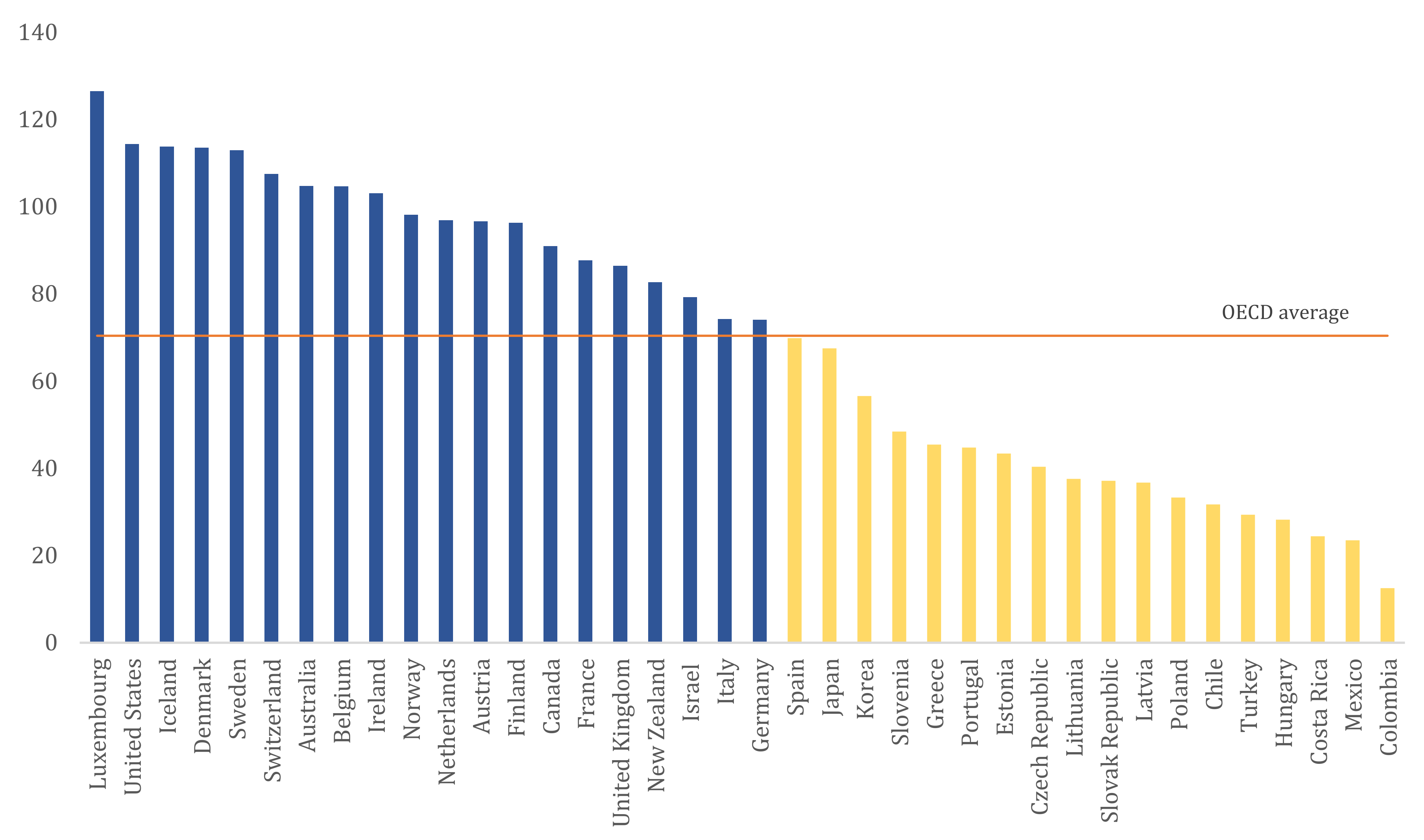
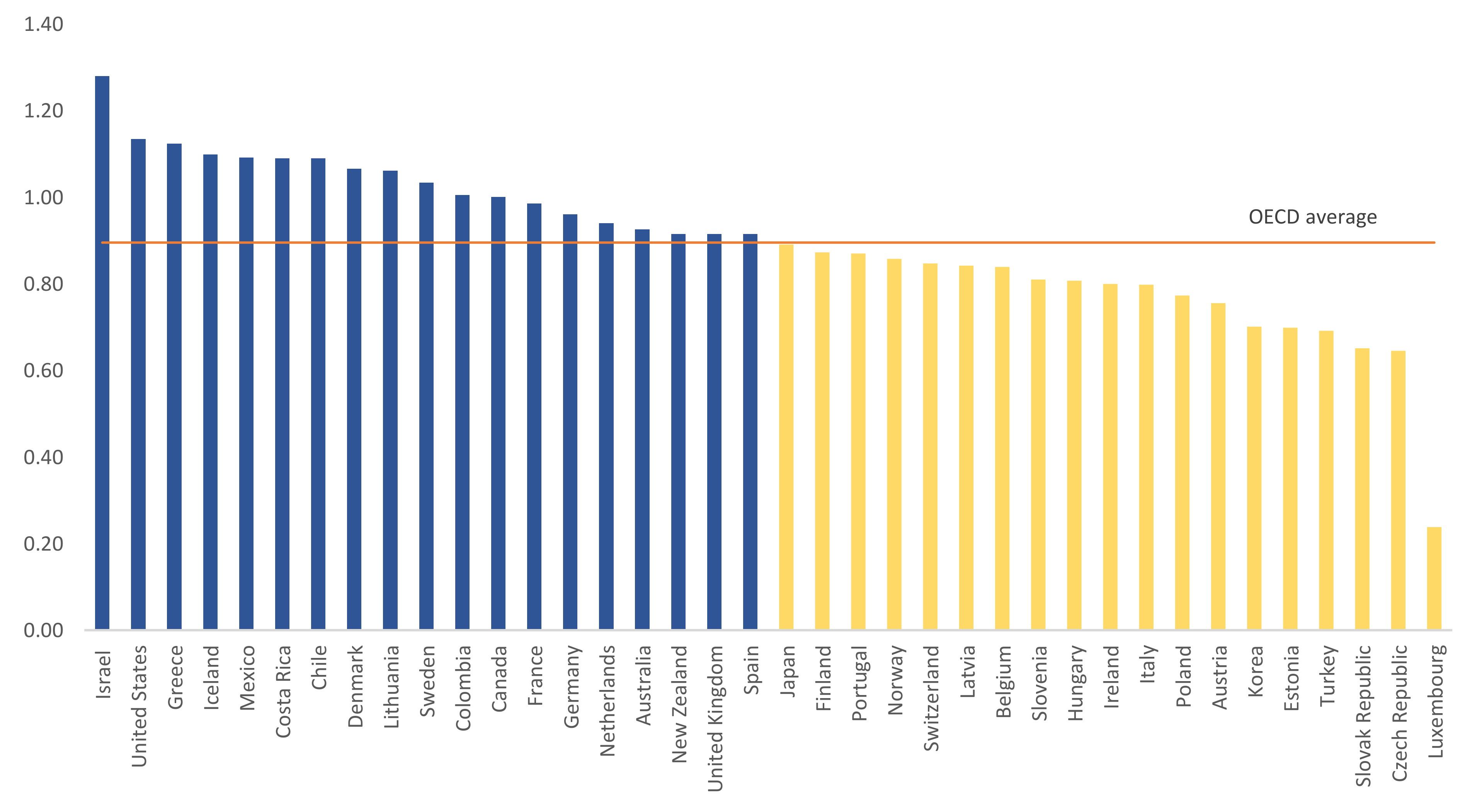
3. Empirical Application
Having determined capital and labour productivities in the previous section, we now proceed in estimating them, within an IO framework, for the 38 OECD countries. In order to do so we use the latest available IO tables provided by the OECD (2021 ed.) for the year 2018. For the labour values per sector, the modulus of the eigenvalues of the input-output coefficients matrix and the sector classification, see the Appendix A.
Figure 1 presents the estimates of labour productivity for each country, with blue bars denoting higher than OECD-average productivity levels, yellow bars lower than average productivity and the orange line the OECD-average. The top five counties in terms of labour productivity are Luxembourg, the United States, Iceland, Denmark and Sweden, while the bottom five are Turkey, Hungary, Costa Rica, Mexico and Colombia. The OECD-average of labour productivity is about 70.4, while all the countries with labour productivity above average are European, plus Australia, New Zealand and the US.
Figure 1.
Labour productivity for the 38 OECD member countries.
Figure 2 depicts the capital productivity of each OECD member country. The top five counties in terms of capital productivity are Israel, the United States, Greece, Iceland and Mexico, while the bottom five include Estonia, Turkey, Slovak Republic, Czech Republic and Luxembourg. The OECD-average of capital productivity is about 0.90, while 10 out of 19 countries with capital productivity above average are once again European.
Figure 2.
Capital productivity for the 38 OECD member countries.
What is interesting to note is that with the exception of Luxemburg, Israel and Colombia, the dispersion in terms of capital productivity is much lower as compared to the dispersion of labour productivity among OECD countries. Excluding the outliers mentioned above, the distance between the top and the lowest country in terms of capital productivity is 74%, while that of labour productivity is 395%, respectively. This implies that the discrepancy in terms of productive efficiency, as reflected in the productivity of capital, is much narrower than labour productivity differentials. Productive efficiency can be considered as the proses of maximizing the production level of a given quantity of inputs used to produce this product [26,27,28], thus in terms of our analytic framework it corresponds to (see, for example [29]). For an empirical verification of the relation between capital productivity and productive efficiency, see [14].
Figure 3 presents the countries with both labour and capital productivity being higher than the OECD-average (the countries with both labour and capital productivity below the average are Czech Republic, Estonia, Hungary, Japan, Korea, Latvia, Poland, Portugal, Slovak Republic, Slovenia and Turkey). Simply put, it presents the countries that should be considered as strongest in terms of economic structure. Indeed, five out of the G7 countries have both labour and capital productivities above the OECD-average, including Canada, France, Germany, the United Kingdom and the United States. In addition, two Scandinavian countries (Denmark and Sweden) and Australia, Iceland, Israel, the Netherlands and New Zealand also appear to have strong economic structures. It appears that the specificities of each economy, its geographical location, institutional and historical, social and political background have a major role in determining the robustness of the economic structure. It is likely of no coincidence that the majority of these countries have undergone a long industrialization process. Alternatively stated, it seems that the overperformance in both productivities is not the outcome of specific policies prescriptions that have been implemented the past one or two decades, but the result of a long-run development. This view is further enhanced when living standards are also taken into account.
Figure 3.
Countries with labour and capital productivity above OECD-average.
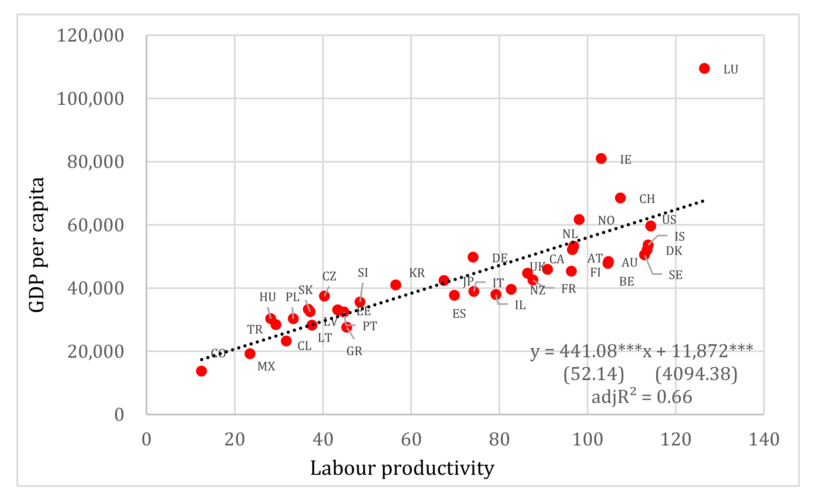
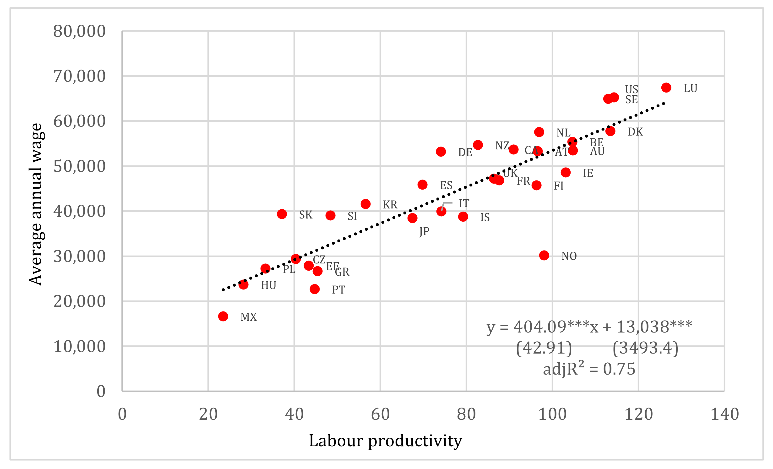
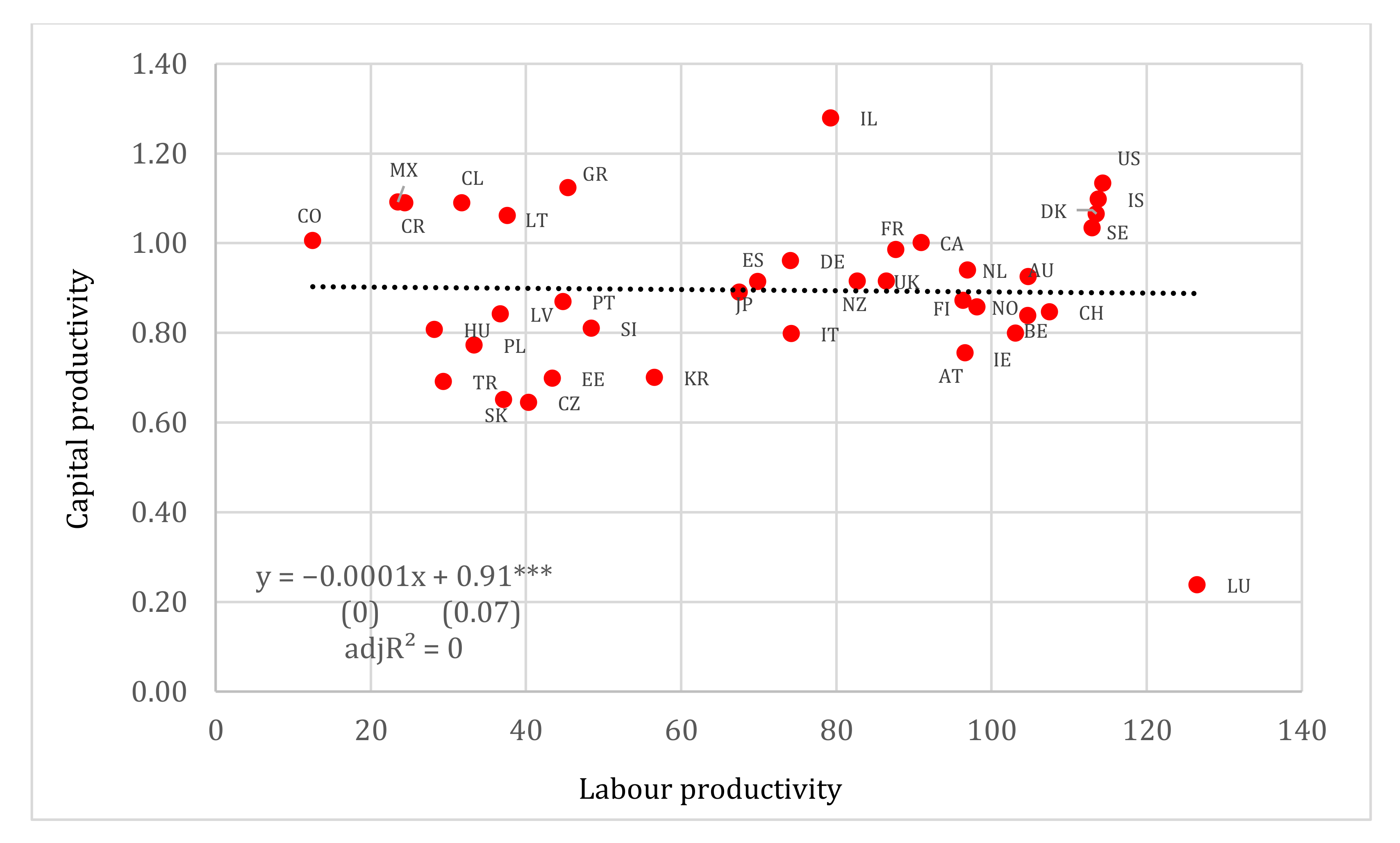
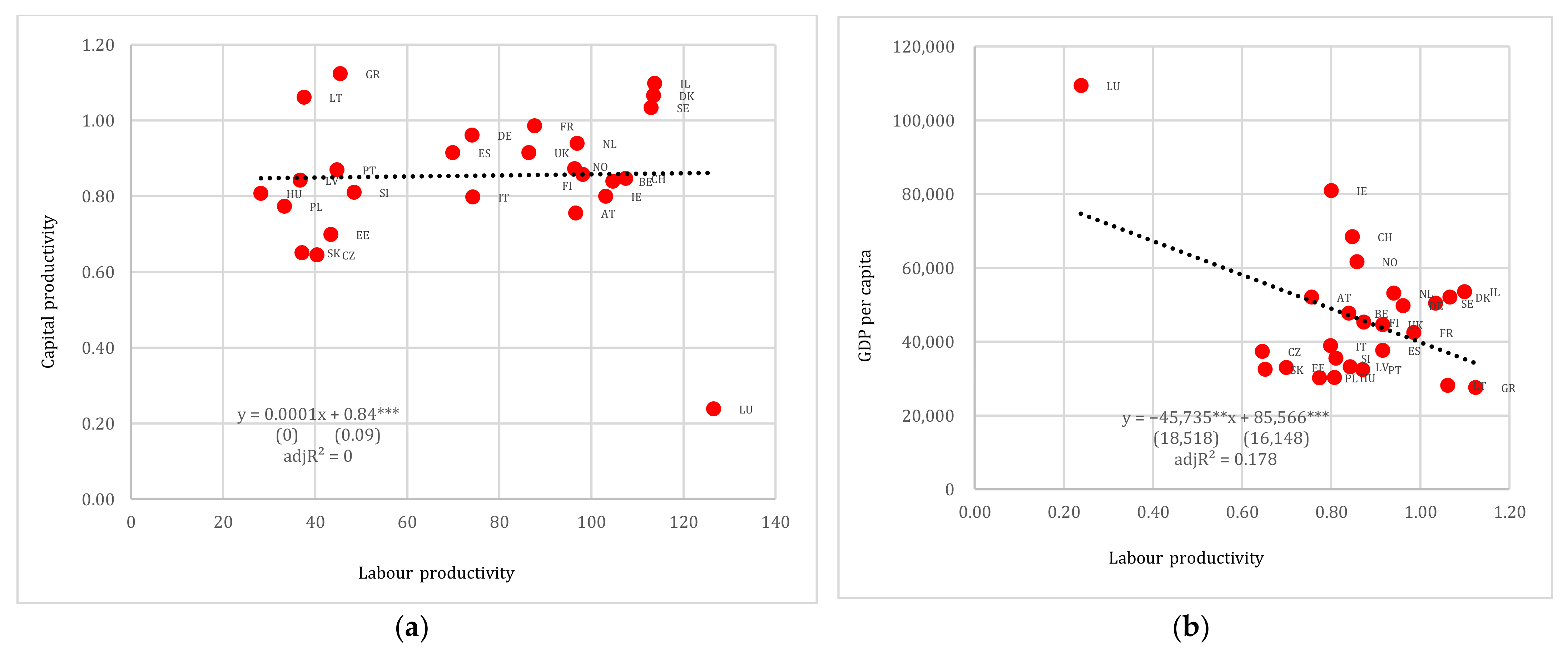
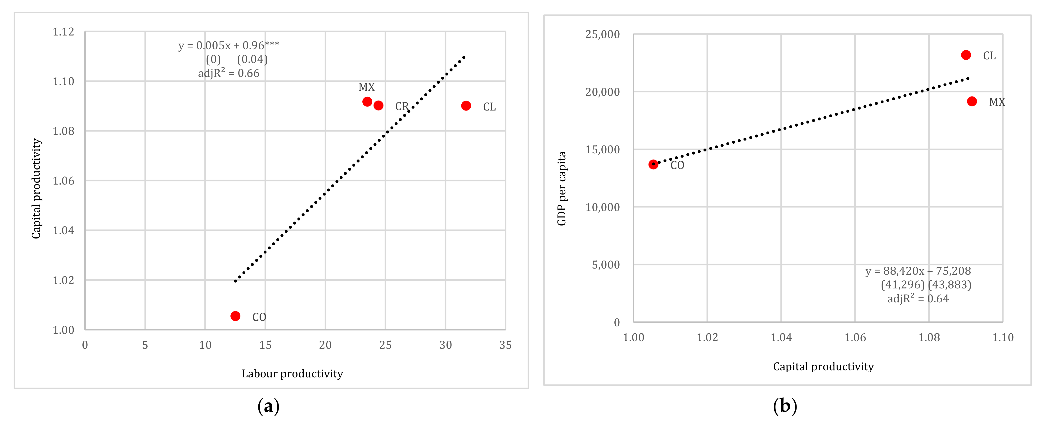
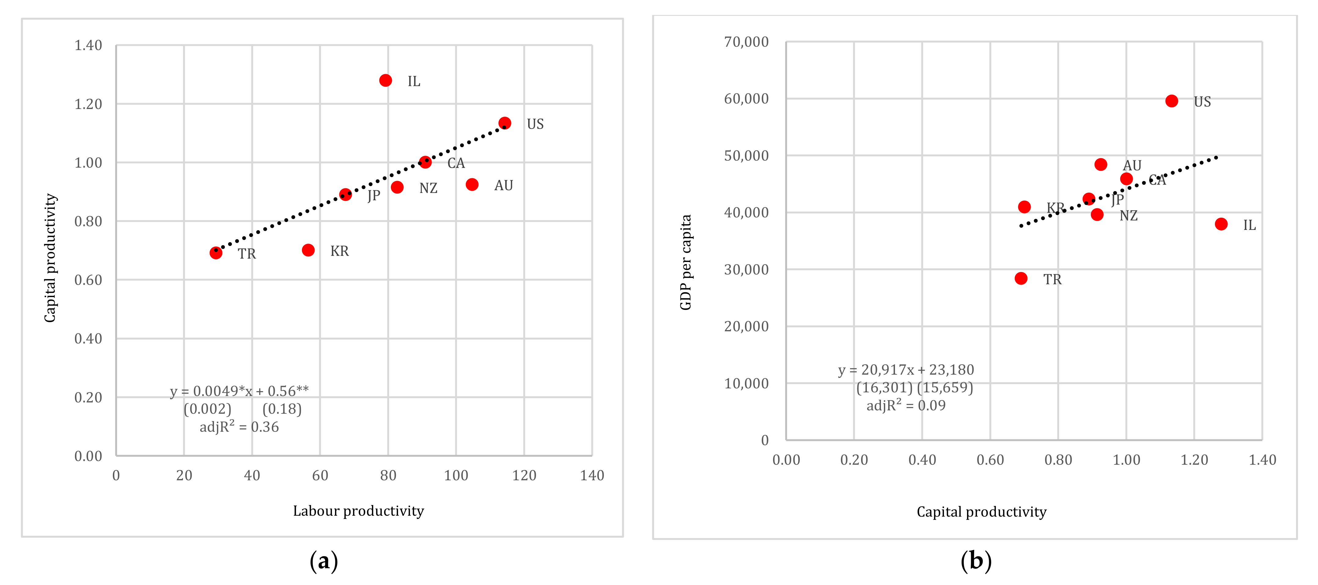
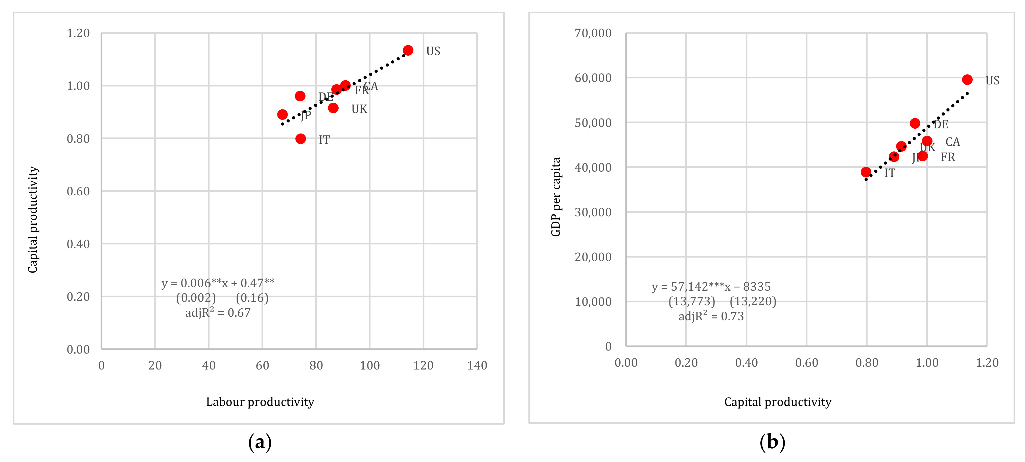
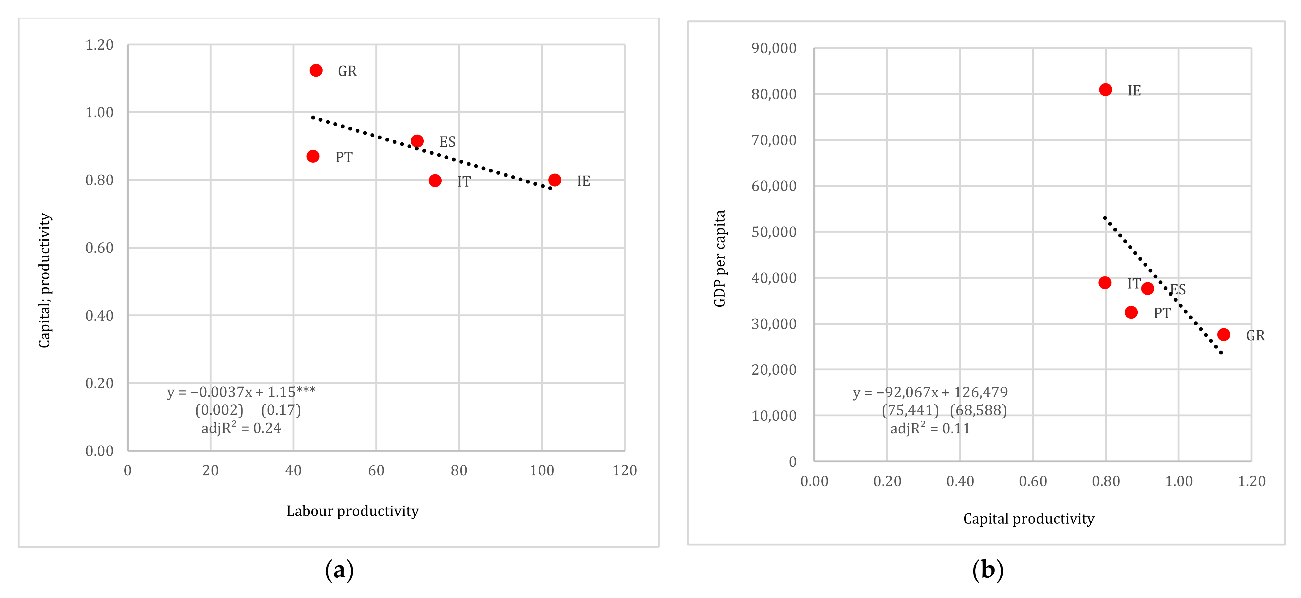
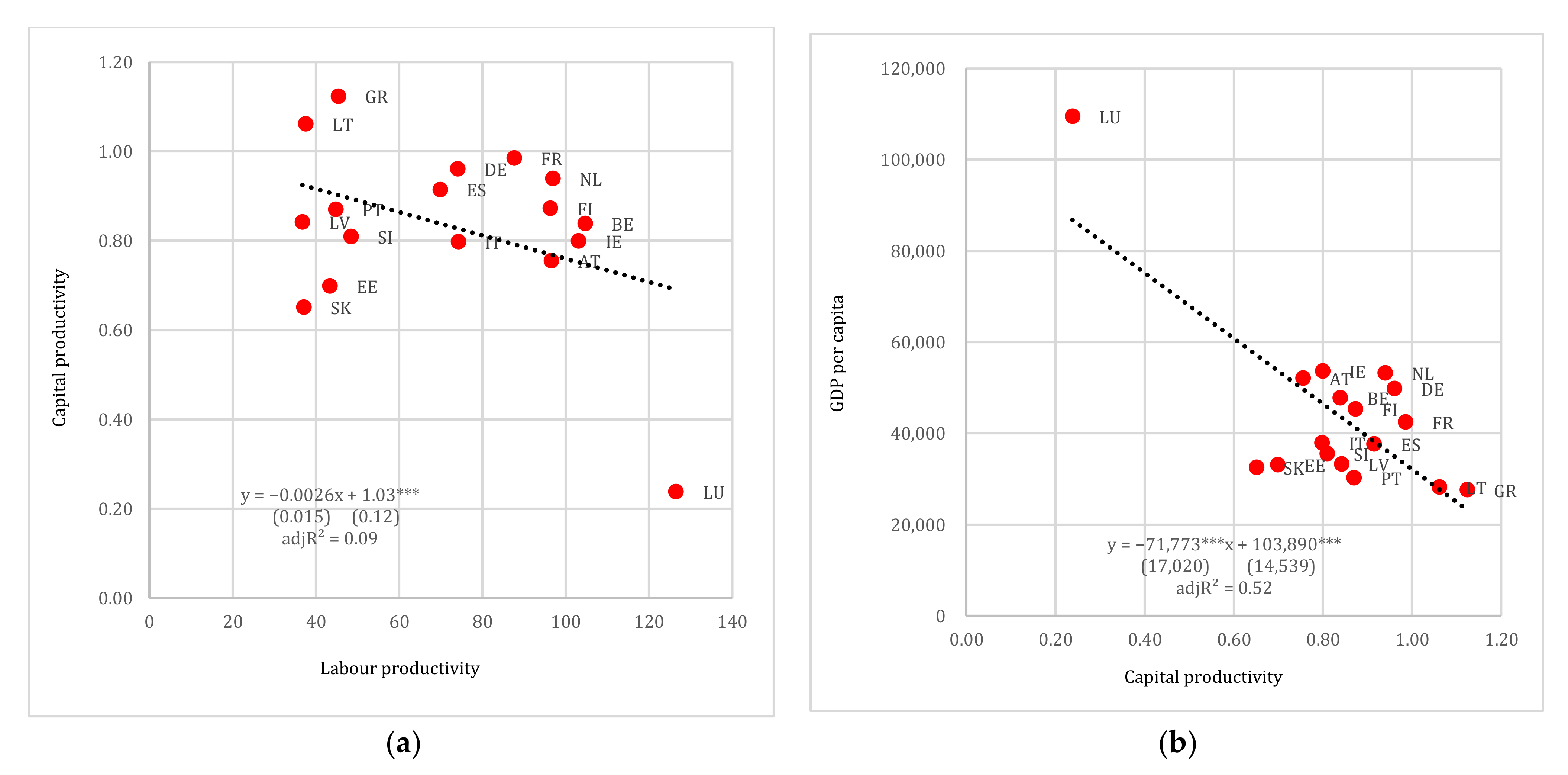
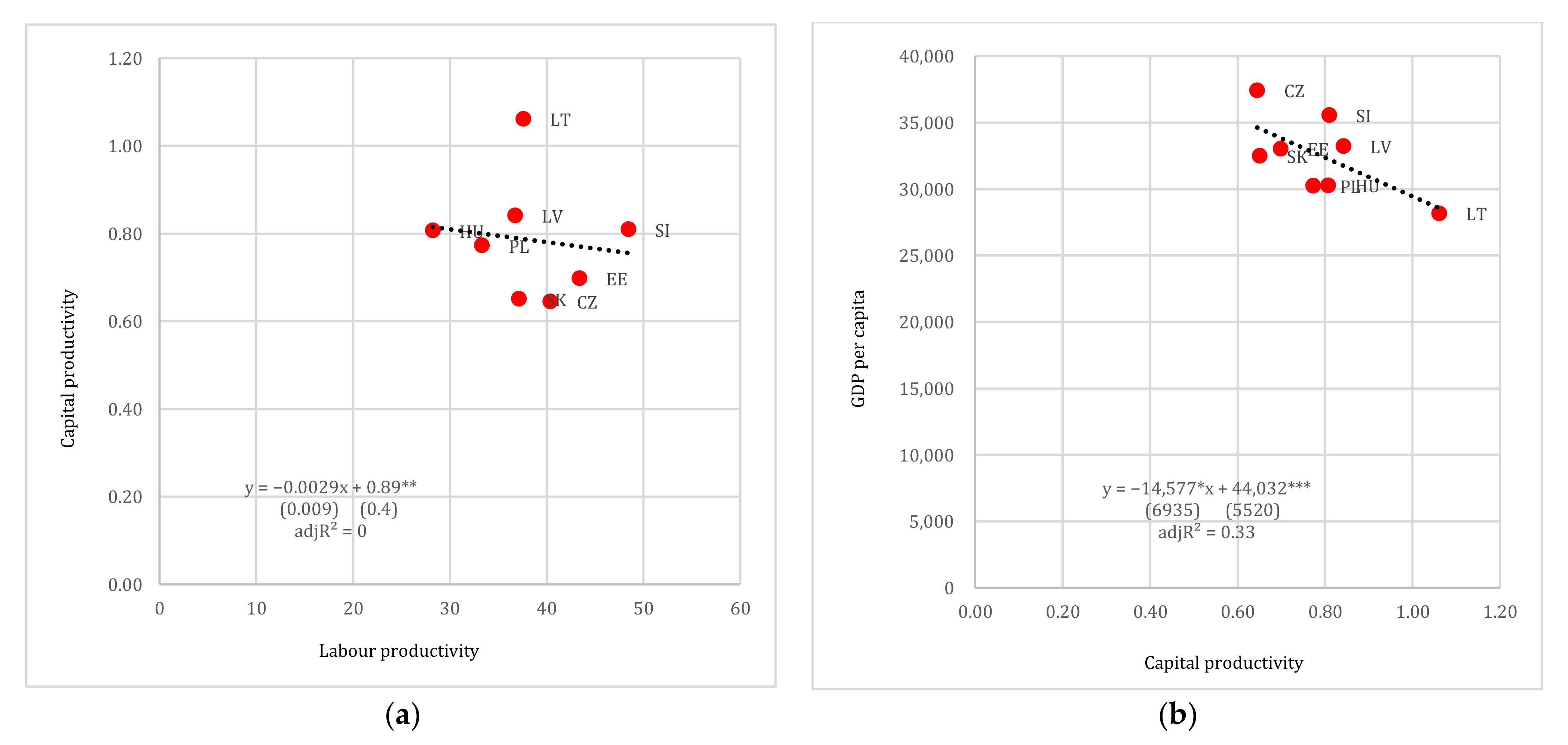
4. Productivity, Economic Efficiency and Living Standards
The measurement of productivity can be considered a key element in the assessment of standards of living. A simple example is the GDP per capita, probably the most common measure of living standards: GDP per capita in an economy varies directly with the measure of productivity. In this sense, measuring productivity helps to better understand the development of living standards. For the relationship between productivity and living standards, see [30,31,32,33].
In what follows, we apply simple linear OLS regressions in order to assess, on the one hand, the relationship between productivity and the GDP per capita and, on the other, productivity and the annual average wages expressed in equivalent purchasing power standards. It should be noted that there are no OECD available data for the GDP per head of population for Costa Rica as well for wages for Chile, Colombia, Iceland, Latvia, Lithuania, New Zealand and Turkey. The data for GDP per head of population and average annual wages are available from https://stats.oecd.org/Index.aspx?DataSet (accessed on 26 February 2022).
Figure 4 models the relationship between GDP per capita (Y) and labour productivity (X). We observe that there is a significant positive linear relation between the two variables. The independent variable is statistically significant, while the standard errors are relatively low. The explanatory power of the regression is also satisfactory. The relation between the two variables becomes even more robust if the outlier Luxemburg (LU) is removed from the sample. In particular, the adjusted R2 increases from 0.66 to 0.74. For higher values of labour productivity, the relationship with GDP per capita is less clear. It is very likely that the relationship is not linear, i.e., a quadratic relation has a much higher explanatory power. Labour productivity appears to have a rather more moderate impact on GDP per capita in richer countries. Nonetheless, further investigation on the matter, i.e., estimating thresholds and turning points, would require more data in order to reach safe conclusions.
Figure 4.
Labour productivity vs. GDP per capita (in USD pps). Note: Standard errors reported in parentheses. *** denotes 1% level of statistical significance.
Testing the relationship between average annual wages (Y) and labour productivity (X), we observe that there is a very strong relationship between the two variables (see Figure 5). The regression has high explanatory power, the coefficients are significant and the standard errors are comparatively low. Again, the removal of the outlier, which in this case is Norway (NO), further increases the robustness of the estimation, as the adjusted R2 rises from 0.75 to 0.85. As expected in this case, the relationship is clearly linear.
Figure 5.
Labour productivity vs. average annual wages (in USD pps). Note: Standard errors reported in parentheses. *** denotes 1% level of statistical significance.
We repeat the same estimating process for the case of capital productivity but fail to find any significant correlation between capital productivity and GDP per capita and capital productivity and average wages. Regarding the relationship between labour and capital productivity we also do not find any significant correlation between them (see Figure 6). For instance, the labour productivity coefficient is practically equal to zero. The latter finding casts doubts over the relationship between labour productivity and productive efficiency, thus supporting the view expressed in the previous section that an analysis, which does not take into account the particular characteristics of each country and its historical and institutional background, can be misleading. Thereby, it is convenient to complement the analysis above with the division of countries according to geographical and economic, financial and political criteria, aiming to generate more homogeneous sub-groups. However, results should be treated as strictly indicative since the size of the sample is reduced considerably.
Figure 6.
Labour vs. capital productivity. Note: Standard errors reported in parentheses. *** denotes 1% level of statistical significance.
As a first attempt, we divide the countries into three groups applying strictly geographical criteria. The first group is consisted of the European countries (i.e., Austria, Belgium, Czech Republic, Denmark, Estonia, Finland, France, Germany, Greece, Hungary, Iceland, Ireland, Italy, Latvia, Lithuania, Luxembourg, Netherlands, Norway, Poland, Portugal, Slovak Republic, Slovenia, Spain, Sweden, Switzerland and the United Kingdom); the second of the Latin American countries (i.e., Chile, Colombia, Costa Rica and Mexico), while the remaining countries form the rest of the world group (i.e., Australia, Canada, Israel, Japan, Korea, New Zealand, Turkey and the United States).
In the case of European countries, regression results suggest that there is no relation between labour and capital productivity (see Figure 7). The removal of Luxemburg (LU) from the regression does not change the overall view, as the trend line remains relatively flat and the explanatory power remarkably low (R2 = 0.14). Regression results are also poor regarding capital productivity as a determinant of GDP per capita, as the standard errors are relatively high and the explanatory power low. Once again, removing the Luxemburg (LU) from the sample yields unsatisfactory results, i.e., the R2 and the capital productivity coefficient are both almost equal to zero.
Figure 7.
(a) Labour productivity vs. capital productivity and (b) capital productivity vs. GDP per capita (in USD pps), Europe. Note: Standard errors reported in parentheses. **, *** denote 5% and 1% levels of statistical significance, respectively.
The sample of the Latin American countries is very small and so the regression outcomes are only demonstrative. Yet, even in this case, the results are quite similar to those in the other cases. Labour productivity does not explain capital productivity, as the coefficient is statistically insignificant (see Figure 8). Removing Colombia (CO) from the regression results in a zero coefficient of labour productivity. Similarly, the relation between capital productivity and GDP per head does not yield satisfactory results, as the coefficient of the explanatory variable is insignificant. Excluding Colombia (CO), the capital productivity coefficient becomes almost equal to zero.
Figure 8.
(a) Labour productivity vs. capital productivity and (b) capital productivity vs. GDP per capita (in USD pps), Latin America. Note: Standard errors reported in parentheses. *** denotes 1% levels of statistical significance.
The third geographical group consists mostly of economies that share some similar characteristics, i.e., most of them are industrialised and developed countries. This is a candidate reason, explaining the significance of labour productivity as a determinant of capital productivity and, in turn, capital productivity as a determinant of GDP per capita (see Figure 9). In the latter case, the regression results do not point to any significant relation between the two variables. However, if Israel (IL) is removed from the sample, both relationships become significant and positive. This result indicates that criteria other than geographical are required so as to retrieve more meaningful outcomes.
Figure 9.
(a) Labour productivity vs. capital productivity and (b) capital productivity vs. GDP per capita (in USD pps), rest of the world. Note: Standard errors reported in parentheses. *, ** denote 10% and 5% levels of statistical significance, respectively.
Following this line of thought, we divide the countries into four distinct sub-groups. The first is formed of the countries that belong to the G7, i.e., Canada, France, Germany, Italy, Japan, the United Kingdom and the United States. The second is consisted of the so-called PIIGS (Portugal, Ireland, Italy, Greece and Spain). During the Global Financial Crisis, these counties were unable to refinance their government debt or to bail out over-indebted banks on their own, thus requiring international financial assistance. The third group is formed of the countries that belong both to the Eurozone and the OECD, while the fourth is consisted of the post-Soviet countries that at the same time are OECD members, i.e., Czech Republic, Estonia, Hungary, Latvia, Lithuania, Poland, Slovak Republic and Slovenia. Therefore, the last group entails countries that have experienced central planning.
As already mentioned above, the labour productivity of all OECD countries does not seem to be related to capital productivity and, therefore, to productive efficiency. However, if we group them in terms of institutional and social characteristics, then we observe cases in which labour productivity may give a satisfactory description of the overall productive efficiency. One such example is the G7 countries (see Figure 10). In this group, there is a strong relationship between the two productivities, efficiency and living standards. The coefficients of the explanatory variable in both regressions are significant, the standard errors are low and the explanatory power adequately high. The industrialization process, in which all member countries have a long tradition and experience, though of a varying degree, is a key element in the transformation of capital efficiency gains to higher living standards. It is of no coincidence that most of the members of this group register higher than the OECD-average values for labour productivity and economic efficiency, as exposed in Figure 3. Note that the correlation is also positive in the case of the South American group (Figure 8), though the sample is small yielding biased results. In fact, with the exclusion of Colombia, which is an outlier, the regression line is flat, implying no correlation between the two productivities.
Figure 10.
(a) Labour productivity vs. capital productivity and (b) capital productivity vs. GDP per capita (in USD pps), G7. Note: Standard errors reported in parentheses. **, *** denote 5% and 1% levels of statistical significance, respectively.
This view is somehow manifested in the case of the second group (see Figure 11). The common element in this group is the high financial fragility of the public and the financial sectors on the run up to the European debt crisis (for instance, see [34,35]) Nevertheless, the economies included have very different institutional and historical backgrounds, varying from moderate industrialization as in the case of Spain, to a marginal industrial structure such as in Greece. In this respect, it does not come as a surprise that the regressions yield insignificant results. These findings are also consistent with the idea of the “multi-speed Europe”, which recognizes the strong developmental and political heterogeneity between the countries of Europe (see also [36,37]).
Figure 11.
(a) Labour productivity vs. capital productivity and (b) capital productivity vs. GDP per capita (in USD pps), PIIGS. Note: Standard errors reported in parentheses. *** denotes 1% levels of statistical significance.
Considering the case of the Eurozone countries, the heterogeneity of this group is reflected to either insignificant econometric results, as is the case between productivity and economic efficiency, or to rather biased results due to the presence of outliers and high standard errors, as is the case between economic efficiency and living standards (see Figure 12). It is noteworthy that lower values of labour productivity are associated with a higher responsiveness of capital productivity to changes in labour productivity. For instance, in Figure 12a countries at the left side of the chart are comparatively poorer and had not undergone the industrialization process that countries on the right side of the panel had. On the contrary, the relation between labour and capital productivities is less clear for the richer sub-group of the Eurozone members. Results in Figure 12b are biased due to the presence of the outlier Luxemburg (LU). Once Luxemburg is removed from the sample, the coefficient of capital productivity becomes statistically insignificant. Finally, in the case of the post-Soviet countries once again the results are unsatisfactory, despite that this group of countries have undergone some form of industrialization during the Soviet era (see Figure 13). This calls for a distinction between market-based and centrally planned industrialization.
Figure 12.
(a) Labour productivity vs. capital productivity and (b) capital productivity vs. GDP per capita (in USD pps), Eurozone. Note: Standard errors reported in parentheses. *** denotes 1% levels of statistical significance.
Figure 13.
(a) Labour productivity vs. capital productivity and (b) capital productivity vs. GDP per capita (in USD pps), post-Soviet. Note: Standard errors reported in parentheses. *, **, *** denote 10%, 5% and 1% levels of statistical significance, respectively.
The above findings corroborate the view that productivity can be considered a satisfactory indicator of the structure and living standards of an economy, but it is not an adequate one. One ought to take into account the particular characteristics of each economy and especially the historical and evolutionary course that characterizes it institutionally, socially and politically. In this context it would prove more efficient to introduce further elements in the analysis that emphasize specifications that lead to varying forms of capitalism [38] or highlight the evolution of institutions that govern economic behaviour [39]. This is clearly manifested in the case of the G7 countries, which have undergone a long industrialization process, and thus, the connection between economic efficiency and higher living standards is more evident. However, for the rest of the countries more is required in order to render economic efficiency, reflected in the capital productivity, meaningful.
Greece stands out as such an example. The country registers the third highest capital productivity among the OECD countries (see Figure 2). This supposedly translates into a strong and sustainable Greek economy. Yet, in the past decade, Greece has become known for the deep recession it experienced, which has been the most intense among OECD countries since 1945. In advance, there is a large gap between labour and capital productivity. As depicted in Figure 1, Greece has a below OECD-average labour productivity. Applying an intersectoral analysis, this could be attributed to the large dependence of the Greek economy on imports and on the importance of the services sector, in conjunction with meager activity in the secondary sector (for alternative explanations on this issue, see [40,41,42,43,44]). At the same time, the shallow industrial structure of the Greek economy was further weakened on the run up to euro (see [45]). Thereby, other factors are likely critical in examining economic efficiency vis-à-vis the higher standards of living.
The example of Greece succinctly points to the need of employing both quantitative and qualitative tools in the analysis, since relying solely on productivity is insufficient and ineffective. Factors that consider the productive structure as an outcome of a long-run developmental path and take into account the institutions that govern the behaviour of economic agents are expected to provide a deeper understanding of the relation between the variables under examination. On top of that, developing the time dimension of the sample, thus generating a panel sample, would allow for a better comparison of the evolution of the productivities across time and space, and their relation to living standards. In conjunction, the above extensions would allow a deeper understanding of the economies at hand and the appropriate re-contextualisation of policy making, thus avoiding ineffective one-size-fits-all policy proposals.
5. Conclusions
In this article, we measure the productivity of capital and labour for all OECD countries, based on a modelling approach that combines principles of the history of economic thought and modern mathematics. We further investigate the relations between productivity, economic efficiency and living standards. In addition to the estimation of the productivities and the verification of the direct relationship between labour productivity and living conditions, the present analysis has shown that there is generally a gap in the relationship between labour productivity and productive efficiency. This gap is somewhat narrowed down by appropriately dividing countries on the basis of geopolitical, institutional and historical criteria.
Our findings emphasize that indicators of productivity cannot be pivotal factors on their own accord but need to be supplemented with information on the historical and institutional path of the economy at hand. Enlarging the time dimension of the sample would also provide a better understanding of the evolution of economic efficiency in relation to living standards. Nonetheless, measuring productivity in order to determine the position of a country in the modern globalized economic system is not an unfounded motivation. Nonetheless, one-size-fits-all measures of productivity are destined to fail in terms of policy proposals as they neglect the specificities and the particularities of each economy, including the sectoral structure, interregional relationships, income distribution, environmental footprint, inter alia.
Author Contributions
Methodology, Z.B., E.K., C.P., N.R. and G.S.; Writing—original draft, Z.B., E.K., C.P., N.R. and G.S.; Writing—review & editing, Z.B., E.K., C.P., N.R. and G.S. All authors have read and agreed to the published version of the manuscript.
Funding
This research received no external funding.
Data Availability Statement
The input-output data used in the research were retrieved from OECD’s database, https://stats.oecd.org (accessed on 26 February 2022).
Conflicts of Interest
The authors declare no conflict of interest.
Appendix A
Table A1.
Labour values per sector of the 38 OECD economies.
Table A1.
Labour values per sector of the 38 OECD economies.
| No. | Australia | Austria | Belgium | Canada | Chile | Colombia | Costa Rica | Czech Republic | Denmark | Estonia | Australia | Austria | Belgium |
|---|---|---|---|---|---|---|---|---|---|---|---|---|---|
| 1 | 0.0104 | 0.0203 | 0.0115 | 0.0113 | 0.0507 | 0.1458 | 0.0689 | 0.0271 | 0.0116 | 0.0221 | 0.0104 | 0.0203 | 0.0115 |
| 2 | 0.0074 | 0.0102 | 0.0065 | 0.0087 | 0.0329 | 0.0675 | 0.063 | 0.0354 | 0.0061 | 0.0168 | 0.0074 | 0.0102 | 0.0065 |
| 3 | 0.0041 | 0.0032 | 0 | 0.0054 | 0.0269 | 0.0274 | 0.0176 | 0.0204 | 0.002 | 0.0171 | 0.0041 | 0.0032 | 0 |
| 4 | 0.0051 | 0.0079 | 0.0075 | 0.0059 | 0.0133 | 0.0254 | 0.0223 | 0.0211 | 0.0061 | 0.0156 | 0.0051 | 0.0079 | 0.0075 |
| 5 | 0.0106 | 0.0061 | 0.0061 | 0.0089 | 0.0105 | 0.0402 | 0.0165 | 0.0262 | 0.0042 | 0.0092 | 0.0106 | 0.0061 | 0.0061 |
| 6 | 0.0106 | 0.0118 | 0.0092 | 0.0113 | 0.0301 | 0.0948 | 0.0427 | 0.0254 | 0.0089 | 0.0226 | 0.0106 | 0.0118 | 0.0092 |
| 7 | 0.0146 | 0.0115 | 0.0095 | 0.0159 | 0.0376 | 0.0988 | 0.0678 | 0.0336 | 0.0089 | 0.0337 | 0.0146 | 0.0115 | 0.0095 |
| 8 | 0.0112 | 0.0114 | 0.0096 | 0.0111 | 0.03 | 0.0803 | 0.054 | 0.0306 | 0.0104 | 0.0227 | 0.0112 | 0.0114 | 0.0096 |
| 9 | 0.0104 | 0.0092 | 0.0087 | 0.0106 | 0.0236 | 0.0708 | 0.0461 | 0.0258 | 0.0098 | 0.0207 | 0.0104 | 0.0092 | 0.0087 |
| 10 | 0.0057 | 0.0045 | 0.0026 | 0.0055 | 0.027 | 0.0292 | 0.0389 | 0.0201 | 0.0025 | 0.0143 | 0.0057 | 0.0045 | 0.0026 |
| 11 | 0.0077 | 0.0083 | 0.0057 | 0.0082 | 0.0264 | 0.0692 | 0.0365 | 0.0193 | 0.0059 | 0.0214 | 0.0077 | 0.0083 | 0.0057 |
| 12 | 0.0083 | 0.0077 | 0.0073 | 0.0096 | 0.0317 | 0.0729 | 0.034 | 0.0197 | 0.004 | 0.0221 | 0.0083 | 0.0077 | 0.0073 |
| 13 | 0.0093 | 0.0093 | 0.0077 | 0.0111 | 0.0327 | 0.1042 | 0.0359 | 0.0231 | 0.008 | 0.0234 | 0.0093 | 0.0093 | 0.0077 |
| 14 | 0.008 | 0.009 | 0.0078 | 0.0098 | 0.0257 | 0.0411 | 0.0257 | 0.0233 | 0.0078 | 0.0191 | 0.008 | 0.009 | 0.0078 |
| 15 | 0.0061 | 0.0075 | 0.0072 | 0.008 | 0.0213 | 0.0457 | 0.0317 | 0.0236 | 0.0085 | 0.0213 | 0.0061 | 0.0075 | 0.0072 |
| 16 | 0.0085 | 0.0094 | 0.0091 | 0.0116 | 0.0406 | 0.0915 | 0.0403 | 0.0276 | 0.0102 | 0.0254 | 0.0085 | 0.0094 | 0.0091 |
| 17 | 0.0097 | 0.0076 | 0.0072 | 0.011 | 0.0306 | 0.0818 | 0.0375 | 0.0214 | 0.0067 | 0.0228 | 0.0097 | 0.0076 | 0.0072 |
| 18 | 0.0108 | 0.008 | 0.0088 | 0.0105 | 0.0411 | 0.0828 | 0.0334 | 0.0246 | 0.0077 | 0.0232 | 0.0108 | 0.008 | 0.0088 |
| 19 | 0.0119 | 0.0085 | 0.0075 | 0.0111 | 0.0314 | 0.1348 | 0.0979 | 0.0257 | 0.0081 | 0.0214 | 0.0119 | 0.0085 | 0.0075 |
| 20 | 0.0106 | 0.0084 | 0.0085 | 0.0105 | 0 | 0.0848 | 0.0366 | 0.0221 | 0.0081 | 0.0183 | 0.0106 | 0.0084 | 0.0085 |
| 21 | 0.0095 | 0.0083 | 0.0073 | 0.0096 | 0.0358 | 0.1026 | 0.0358 | 0.0238 | 0.0092 | 0.024 | 0.0095 | 0.0083 | 0.0073 |
| 22 | 0.018 | 0.0102 | 0.0093 | 0.0139 | 0.0323 | 0.0652 | 0.0287 | 0.0279 | 0.0076 | 0.0253 | 0.018 | 0.0102 | 0.0093 |
| 23 | 0.0052 | 0.0051 | 0.0042 | 0.0052 | 0.0156 | 0.0249 | 0.019 | 0.0154 | 0.004 | 0.0125 | 0.0052 | 0.0051 | 0.0042 |
| 24 | 0.0066 | 0.0069 | 0.0073 | 0.0093 | 0.0238 | 0.0449 | 0.0255 | 0.0237 | 0.0064 | 0.018 | 0.0066 | 0.0069 | 0.0073 |
| 25 | 0.0099 | 0.01 | 0.0089 | 0.0115 | 0.0332 | 0.0632 | 0.0401 | 0.0263 | 0.0089 | 0.0221 | 0.0099 | 0.01 | 0.0089 |
| 26 | 0.0126 | 0.012 | 0.0092 | 0.015 | 0.0421 | 0.1079 | 0.0525 | 0.0255 | 0.0104 | 0.0224 | 0.0126 | 0.012 | 0.0092 |
| 27 | 0.0125 | 0.0097 | 0.0089 | 0.011 | 0.0348 | 0.062 | 0.0348 | 0.0238 | 0.0094 | 0.023 | 0.0125 | 0.0097 | 0.0089 |
| 28 | 0.0079 | 0.0086 | 0.0054 | 0.0104 | 0.0303 | 0.0632 | 0.0343 | 0.0237 | 0.0068 | 0.0182 | 0.0079 | 0.0086 | 0.0054 |
| 29 | 0.0082 | 0.0081 | 0.007 | 0.0094 | 0.0342 | 0.1048 | 0.0849 | 0.0175 | 0.0062 | 0.0205 | 0.0082 | 0.0081 | 0.007 |
| 30 | 0.0073 | 0.0072 | 0.0079 | 0.0115 | 0.0256 | 0.0971 | 0.0225 | 0.0203 | 0.0082 | 0.0164 | 0.0073 | 0.0072 | 0.0079 |
| 31 | 0.0136 | 0.013 | 0.0114 | 0.0154 | 0.0492 | 0.1008 | 0.0297 | 0.0408 | 0.0166 | 0.0376 | 0.0136 | 0.013 | 0.0114 |
| 32 | 0.0176 | 0.0126 | 0.0121 | 0.0229 | 0.0454 | 0.1001 | 0.0485 | 0.0326 | 0.0165 | 0.032 | 0.0176 | 0.0126 | 0.0121 |
| 33 | 0.01 | 0.0095 | 0.0077 | 0.0123 | 0.0328 | 0.0649 | 0.0372 | 0.0165 | 0.0085 | 0.0262 | 0.01 | 0.0095 | 0.0077 |
| 34 | 0.0075 | 0.0062 | 0.0053 | 0.0072 | 0.0226 | 0.0371 | 0.0188 | 0.0128 | 0.0062 | 0.0141 | 0.0075 | 0.0062 | 0.0053 |
| 35 | 0.0091 | 0.0098 | 0.0074 | 0.0114 | 0.0265 | 0.0511 | 0.0141 | 0.0165 | 0.0082 | 0.0185 | 0.0091 | 0.0098 | 0.0074 |
| 36 | 0.005 | 0.0083 | 0.0054 | 0.01 | 0.0163 | 0.0297 | 0.0183 | 0.0142 | 0.0052 | 0.0132 | 0.005 | 0.0083 | 0.0054 |
| 37 | 0.0028 | 0.0037 | 0.0021 | 0.0037 | 0.0081 | 0.013 | 0.008 | 0.0125 | 0.0033 | 0.0081 | 0.0028 | 0.0037 | 0.0021 |
| 38 | 0.0103 | 0.0113 | 0.0092 | 0.0126 | 0.02 | 0.0999 | 0.0192 | 0.0255 | 0.0083 | 0.02 | 0.0103 | 0.0113 | 0.0092 |
| No. | Greece | Hungary | Iceland | Ireland | Israel | Italy | Japan | Korea | Latvia | Lithuania | Luxembourg | Mexico | Netherlands |
| 1 | 0.0467 | 0.0304 | 0.0105 | 0.0146 | 0.0126 | 0.0182 | 0.0336 | 0.0311 | 0.0365 | 0.0394 | 0.0138 | 0.0587 | 0.0114 |
| 2 | 0.0251 | 0.0513 | 0.0057 | 0.0103 | 0.0096 | 0.0183 | 0.0442 | 0.0404 | 0.0325 | 0.0245 | 0 | 0.0524 | 0.008 |
| 3 | 0.0115 | 0.0161 | 0.0048 | 0.0055 | 0.002 | 0.0076 | 0.0066 | 0.012 | 0.0147 | 0.0193 | 0 | 0.007 | 0.0022 |
| 4 | 0.0154 | 0.0293 | 0.0069 | 0.0063 | 0.0028 | 0.0119 | 0.0135 | 0.0139 | 0.0206 | 0.0267 | 0.0063 | 0.0184 | 0.0063 |
| 5 | 0.0256 | 0.0195 | 0.0058 | 0.0058 | 0.0032 | 0.0091 | 0.0137 | 0.0376 | 0.0187 | 0.0215 | 0.0081 | 0.0301 | 0.0055 |
| 6 | 0.0258 | 0.0328 | 0.0082 | 0.0081 | 0.0133 | 0.0134 | 0.0184 | 0.0225 | 0.0305 | 0.0254 | 0.0117 | 0.0323 | 0.0098 |
| 7 | 0.0281 | 0.0535 | 0.0107 | 0.0145 | 0.013 | 0.0134 | 0.0248 | 0.0186 | 0.0423 | 0.0341 | 0.007 | 0.0571 | 0.0105 |
| 8 | 0.0379 | 0.0426 | 0.0099 | 0.0103 | 0.0115 | 0.0151 | 0.0196 | 0.0197 | 0.0277 | 0.0297 | 0.0095 | 0.0502 | 0.0104 |
| 9 | 0.0215 | 0.0352 | 0.0113 | 0.0131 | 0.0121 | 0.0123 | 0.0149 | 0.0156 | 0.0293 | 0.0219 | 0.0118 | 0.032 | 0.0096 |
| 10 | 0.0128 | 0.0196 | 0.0016 | 0.0019 | 0.0039 | 0.0086 | 0.0112 | 0.0106 | 0.012 | 0.0192 | 0 | 0.0132 | 0.0044 |
| 11 | 0.0135 | 0.019 | 0.0082 | 0.0041 | 0.0069 | 0.0092 | 0.0103 | 0.0111 | 0.0259 | 0.0191 | 0.0082 | 0.02 | 0.0069 |
| 12 | 0.0159 | 0.0207 | 0.0405 | 0.0036 | 0.0071 | 0.0094 | 0.0081 | 0.012 | 0.0254 | 0.0154 | 0.0062 | 0.0308 | 0.0073 |
| 13 | 0.017 | 0.0255 | 0.0082 | 0.0079 | 0.0094 | 0.0113 | 0.0152 | 0.0144 | 0.029 | 0.0202 | 0.0076 | 0.0327 | 0.009 |
| 14 | 0.0171 | 0.0252 | 0.0071 | 0.0058 | 0.0075 | 0.012 | 0.0126 | 0.0141 | 0.0235 | 0.028 | 0.0071 | 0.0301 | 0.0094 |
| 15 | 0.0142 | 0.0236 | 0.0063 | 0.0092 | 0.042 | 0.0111 | 0.0091 | 0.0126 | 0.0345 | 0.0257 | 0.0067 | 0.0173 | 0.0081 |
| 16 | 0.0214 | 0.034 | 0.0085 | 0.0085 | 0.012 | 0.0127 | 0.0134 | 0.0151 | 0.0315 | 0.0268 | 0.0088 | 0.0338 | 0.01 |
| 17 | 0.0169 | 0.0287 | 0.0081 | 0.0033 | 0.0088 | 0.0109 | 0.0103 | 0.0089 | 0.0222 | 0.0203 | 0.0081 | 0.0336 | 0.0111 |
| 18 | 0.0182 | 0.0304 | 0.0077 | 0.0073 | 0.0125 | 0.0116 | 0.0107 | 0.0132 | 0.0273 | 0.0265 | 0.0098 | 0.0312 | 0.0084 |
| 19 | 0.0204 | 0.0303 | 0.007 | 0.003 | 0.0113 | 0.0112 | 0.0113 | 0.0142 | 0.03 | 0.0227 | 0.0075 | 0.0322 | 0.0084 |
| 20 | 0.0246 | 0.0264 | 0.0041 | 0.0101 | 0.012 | 0.011 | 0.0103 | 0.0137 | 0.0283 | 0.0235 | 0.0079 | 0.0253 | 0.0082 |
| 21 | 0.0137 | 0.0306 | 0.004 | 0.0064 | 0.0128 | 0.0111 | 0.0112 | 0.0149 | 0.0343 | 0.0216 | 0.0048 | 0.029 | 0.0103 |
| 22 | 0.0318 | 0.0376 | 0.0076 | 0.0027 | 0.0114 | 0.0132 | 0.0161 | 0.0193 | 0.0326 | 0.0269 | 0.0101 | 0.0455 | 0.0132 |
| 23 | 0.0087 | 0.0231 | 0.0038 | 0.0042 | 0.0051 | 0.0071 | 0.0106 | 0.0099 | 0.0182 | 0.0188 | 0.0042 | 0.0107 | 0.0054 |
| 24 | 0.0123 | 0.0353 | 0.0058 | 0.0054 | 0.0163 | 0.0117 | 0.0063 | 0.0137 | 0.0257 | 0.0291 | 0.0078 | 0.0289 | 0.0085 |
| 25 | 0.0364 | 0.0357 | 0.0076 | 0.0104 | 0.0124 | 0.0148 | 0.0163 | 0.0179 | 0.028 | 0.0276 | 0.009 | 0.0418 | 0.0105 |
| 26 | 0.0244 | 0.0356 | 0.0098 | 0.0092 | 0.0124 | 0.0138 | 0.0161 | 0.0232 | 0.0291 | 0.0258 | 0.0074 | 0.0244 | 0.0119 |
| 27 | 0.0263 | 0.0296 | 0.009 | 0.0126 | 0.0138 | 0.0111 | 0.016 | 0.0248 | 0.0231 | 0.0191 | 0.0073 | 0.0301 | 0.0113 |
| 28 | 0.012 | 0.0495 | 0.0065 | 0.0149 | 0.0072 | 0.0106 | 0.0128 | 0.0152 | 0.0201 | 0.0173 | 0.0077 | 0.0232 | 0.0084 |
| 29 | 0.0137 | 0.0174 | 0.0064 | 0.0061 | 0.0073 | 0.0099 | 0.0128 | 0.0123 | 0.0196 | 0.0226 | 0.0075 | 0.0262 | 0.0077 |
| 30 | 0.0142 | 0.0288 | 0.0075 | 0.0081 | 0.0214 | 0.0113 | 0.0124 | 0.0179 | 0.0227 | 0.018 | 0.0065 | 0.0328 | 0.0085 |
| 31 | 0.0221 | 0.0601 | 0.0162 | 0.0136 | 0.0189 | 0.0175 | 0.0219 | 0.0164 | 0.0321 | 0.0398 | 0.0066 | 0.0362 | 0.0178 |
| 32 | 0.0332 | 0.0455 | 0.0122 | 0.0206 | 0.0173 | 0.0173 | 0.0246 | 0.0307 | 0.0359 | 0.033 | 0.0138 | 0.0466 | 0.0179 |
| 33 | 0.026 | 0.0267 | 0.0121 | 0.0031 | 0.0119 | 0.0107 | 0.0122 | 0.018 | 0.0255 | 0.0249 | 0.007 | 0.0291 | 0.0115 |
| 34 | 0.0102 | 0.0203 | 0.0056 | 0.0038 | 0.0055 | 0.0069 | 0.0085 | 0.0098 | 0.0147 | 0.0146 | 0.0052 | 0.0146 | 0.0063 |
| 35 | 0.0202 | 0.0266 | 0.007 | 0.0053 | 0.0073 | 0.0115 | 0.0133 | 0.0105 | 0.0233 | 0.0212 | 0.0064 | 0.0448 | 0.0097 |
| 36 | 0.0102 | 0.0215 | 0.0045 | 0.0049 | 0.0095 | 0.0078 | 0.0107 | 0.0106 | 0.0162 | 0.0197 | 0.0038 | 0.0177 | 0.0054 |
| 37 | 0.0024 | 0.013 | 0.0022 | 0.0017 | 0.0018 | 0.002 | 0.0037 | 0.0071 | 0.0094 | 0.0095 | 0.0024 | 0.0058 | 0.0042 |
| 38 | 0.0317 | 0.0293 | 0.0081 | 0.007 | 0.0111 | 0.0131 | 0.0184 | 0.0136 | 0.0298 | 0.0293 | 0.0073 | 0.0262 | 0.0112 |
| No. | New Zealand | Norway | Poland | Portugal | Slovak Republic | Slovenia | Spain | Sweden | Switzerland | Turkey | United Kingdom | United States | |
| 1 | 0.013 | 0.0132 | 0.0643 | 0.0561 | 0.0263 | 0.0423 | 0.0172 | 0.0106 | 0.0191 | 0.0829 | 0.0167 | 0.0096 | |
| 2 | 0.0066 | 0.005 | 0.0562 | 0.0295 | 0.0376 | 0.0263 | 0.0177 | 0.007 | 0.0155 | 0.1502 | 0.0156 | 0.0103 | |
| 3 | 0.0067 | 0.0011 | 0.0213 | 0 | 0.0365 | 0.0153 | 0.0021 | 0.0058 | 0.0038 | 0.03 | 0.0045 | 0.0032 | |
| 4 | 0.0039 | 0.0059 | 0.0229 | 0.0163 | 0.0222 | 0.0169 | 0.0107 | 0.0044 | 0.0082 | 0.0197 | 0.01 | 0.0052 | |
| 5 | 0.0129 | 0.0067 | 0.0303 | 0.0198 | 0.0071 | 0.0141 | 0.0109 | 0.0072 | 0.0052 | 0.017 | 0.0127 | 0.0064 | |
| 6 | 0.012 | 0.0085 | 0.0347 | 0.0291 | 0.028 | 0.0241 | 0.0149 | 0.0092 | 0.0091 | 0.0508 | 0.0122 | 0.0085 | |
| 7 | 0.0166 | 0.0087 | 0.0448 | 0.0304 | 0.0362 | 0.0233 | 0.0128 | 0.0102 | 0.0082 | 0.0403 | 0.0114 | 0.0104 | |
| 8 | 0.0142 | 0.0092 | 0.0392 | 0.0293 | 0.0298 | 0.0244 | 0.0166 | 0.0099 | 0.0096 | 0.0447 | 0.0158 | 0.0091 | |
| 9 | 0.0123 | 0.0076 | 0.0257 | 0.0213 | 0.0231 | 0.0196 | 0.0135 | 0.0074 | 0.0084 | 0.031 | 0.012 | 0.0078 | |
| 10 | 0.006 | 0.0026 | 0.0201 | 0.004 | 0.0276 | 0.0136 | 0.0048 | 0.0061 | 0.004 | 0.024 | 0.0054 | 0.0032 | |
| 11 | 0.0092 | 0.0054 | 0.0243 | 0.0179 | 0.0196 | 0.0165 | 0.0115 | 0.0071 | 0.0069 | 0.0203 | 0.0092 | 0.0051 | |
| 12 | 0.012 | 0.004 | 0.0198 | 0.0159 | 0.0246 | 0.0128 | 0.0098 | 0.0058 | 0.0037 | 0.0342 | 0.0068 | 0.0037 | |
| 13 | 0.0103 | 0.008 | 0.0272 | 0.0185 | 0.0231 | 0.0194 | 0.0133 | 0.0091 | 0.007 | 0.029 | 0.0129 | 0.0077 | |
| 14 | 0.0099 | 0.0068 | 0.0264 | 0.0199 | 0.0239 | 0.0177 | 0.0129 | 0.0088 | 0.007 | 0.0296 | 0.0113 | 0.0066 | |
| 15 | 0.0092 | 0.0054 | 0.0267 | 0.0177 | 0.0222 | 0.0183 | 0.0111 | 0.0072 | 0.0068 | 0.0199 | 0.0116 | 0.0064 | |
| 16 | 0.013 | 0.008 | 0.0278 | 0.0238 | 0.0262 | 0.0205 | 0.0145 | 0.0095 | 0.0079 | 0.0323 | 0.0131 | 0.0084 | |
| 17 | 0.0092 | 0.0068 | 0.0285 | 0.0222 | 0.0241 | 0.0169 | 0.0131 | 0.0076 | 0.006 | 0.0195 | 0.0085 | 0.0045 | |
| 18 | 0.0097 | 0.0074 | 0.0277 | 0.021 | 0.0258 | 0.0193 | 0.0129 | 0.0087 | 0.0066 | 0.03 | 0.012 | 0.0067 | |
| 19 | 0.0116 | 0.0077 | 0.0297 | 0.021 | 0.025 | 0.0196 | 0.0134 | 0.0077 | 0.0067 | 0.0307 | 0.0105 | 0.0072 | |
| 20 | 0.011 | 0.0073 | 0.0277 | 0.019 | 0.0224 | 0.0179 | 0.0128 | 0.0072 | 0.007 | 0.0231 | 0.0099 | 0.0071 | |
| 21 | 0.0131 | 0.0074 | 0.0317 | 0.022 | 0.0264 | 0.0208 | 0.0119 | 0.0071 | 0.0069 | 0.0165 | 0.0102 | 0.0056 | |
| 22 | 0.0253 | 0.0083 | 0.0338 | 0.0265 | 0.0283 | 0.0216 | 0.0148 | 0.01 | 0.0073 | 0.0348 | 0.012 | 0.0073 | |
| 23 | 0.0058 | 0.0022 | 0.0177 | 0.0051 | 0.0197 | 0.0132 | 0.0062 | 0.0049 | 0.006 | 0.0229 | 0.0068 | 0.0034 | |
| 24 | 0.0085 | 0.0063 | 0.0233 | 0.0198 | 0.0259 | 0.0204 | 0.0128 | 0.0085 | 0.0082 | 0.0268 | 0.0074 | 0.0073 | |
| 25 | 0.0137 | 0.008 | 0.0274 | 0.0261 | 0.0224 | 0.0213 | 0.0142 | 0.0099 | 0.0085 | 0.0304 | 0.0125 | 0.009 | |
| 26 | 0.0153 | 0.0096 | 0.0249 | 0.0229 | 0.0291 | 0.0204 | 0.0171 | 0.0099 | 0.0064 | 0.0353 | 0.0148 | 0.0097 | |
| 27 | 0.0114 | 0.0082 | 0.0246 | 0.0193 | 0.021 | 0.0182 | 0.0143 | 0.0095 | 0.0085 | 0.0223 | 0.0151 | 0.0081 | |
| 28 | 0.0109 | 0.0065 | 0.034 | 0.0188 | 0.0206 | 0.0138 | 0.0105 | 0.0085 | 0.0049 | 0.0113 | 0.0061 | 0.0067 | |
| 29 | 0.0095 | 0.0064 | 0.0244 | 0.0131 | 0.0238 | 0.0186 | 0.0114 | 0.0069 | 0.0069 | 0.0133 | 0.0091 | 0.0064 | |
| 30 | 0.0099 | 0.0077 | 0.0209 | 0.013 | 0.0206 | 0.0132 | 0.0115 | 0.0082 | 0.0077 | 0.018 | 0.0118 | 0.0104 | |
| 31 | 0.0179 | 0.0118 | 0.0486 | 0.0246 | 0.0391 | 0.0259 | 0.0255 | 0.0123 | 0.0119 | 0.0348 | 0.0149 | 0.0114 | |
| 32 | 0.021 | 0.0125 | 0.0414 | 0.0263 | 0.0469 | 0.0282 | 0.0169 | 0.0154 | 0.0145 | 0.0528 | 0.0211 | 0.0165 | |
| 33 | 0.014 | 0.0078 | 0.0222 | 0.0183 | 0.0206 | 0.0223 | 0.0123 | 0.0064 | 0.0085 | 0.0253 | 0.0096 | 0.0051 | |
| 34 | 0.0126 | 0.0044 | 0.0189 | 0.0135 | 0.0133 | 0.0124 | 0.0086 | 0.0046 | 0.0049 | 0.0202 | 0.0064 | 0.0045 | |
| 35 | 0.0222 | 0.007 | 0.0221 | 0.0203 | 0.0193 | 0.0187 | 0.0152 | 0.0068 | 0.0065 | 0.0146 | 0.0109 | 0.0056 | |
| 36 | 0.0075 | 0.0034 | 0.02 | 0.0105 | 0.0172 | 0.0138 | 0.0085 | 0.0052 | 0.0046 | 0.0176 | 0.0087 | 0.0048 | |
| 37 | 0.0041 | 0.0029 | 0.0132 | 0.0036 | 0.0074 | 0.0045 | 0.003 | 0.0042 | 0.0027 | 0.0134 | 0.0033 | 0.0026 | |
| 38 | 0.0116 | 0.0077 | 0.0217 | 0.0224 | 0.022 | 0.0219 | 0.0155 | 0.0086 | 0.0079 | 0.0387 | 0.0128 | 0.0068 | |
Note: The labour values are estimated assuming a single production case without fixed capital.
Table A2.
Sector Classification of the 38 OECD economies.
Table A2.
Sector Classification of the 38 OECD economies.
| No. | Nomenclature |
|---|---|
| 1 | D01T03: Agriculture, forestry and fishing |
| 2 | D05T06: Mining and extraction of energy producing products |
| 3 | D07T08: Mining and quarrying of non-energy producing products |
| 4 | D09: Mining support service activities |
| 5 | D10T12: Food products, beverages and tobacco |
| 6 | D13T15: Textiles, wearing apparel, leather and related products |
| 7 | D16: Wood and products of wood and cork |
| 8 | D17T18: Paper products and printing |
| 9 | D19: Coke and refined petroleum products |
| 10 | D20T21: Chemicals and pharmaceutical products |
| 11 | D22: Rubber and plastic products |
| 12 | D23: Other non-metallic mineral products |
| 13 | D24: Basic metals |
| 14 | D25: Fabricated metal products |
| 15 | D26: Computer, electronic and optical products |
| 16 | D27: Electrical equipment |
| 17 | D28: Machinery and equipment, nec |
| 18 | D29: Motor vehicles, trailers and semi-trailers |
| 19 | D30: Other transport equipment |
| 20 | D31T33: Other manufacturing; repair and installation of machinery and equipment |
| 21 | D35T39: Electricity, gas, water supply, sewerage, waste and remediation services |
| 22 | D41T43: Construction |
| 23 | D45T47: Wholesale and retail trade; repair of motor vehicles |
| 24 | D49T53: Transportation and storage |
| 25 | D55T56: Accomodation and food services |
| 26 | D58T60: Publishing, audiovisual and broadcasting activities |
| 27 | D61: Telecommunications |
| 28 | D62T63: IT and other information services |
| 29 | D64T66: Financial and insurance activities |
| 30 | D68: Real estate activities |
| 31 | D69T82: Other business sector services |
| 32 | D84: Public admin. and defence; compulsory social security |
| 33 | D85: Education |
| 34 | D86T88: Human health and social work |
| 35 | D90T96: Arts, entertainment, recreation and other service activities |
| 36 | D97T98: Private households with employed persons |
| 37 | D01T03: Agriculture, forestry and fishing |
| 38 | D05T06: Mining and extraction of energy producing products |


Figure A1.
The modulus of the eigenvalues of the input-output coefficients matrix of the 38 OECD economies.
References
- Krämer, H.M.; Kurz, H.D. La “Productivité”: Histoire d’une Notion Complexe; Plateforme de Politique Économique: Berne, Switzerland, 2021; Available online: https://dievolkswirtschaft.ch/fr/2021/10/la-productivite-histoire-dune-notion-complexe/ (accessed on 10 January 2022).
- Kurz, H.D.; Salvadori, N. Theories of economic growth: Old and new. In The Theory of Economic Growth: A “Classical” Perspective; Salvadori, N., Ed.; Edward Elgar: Northampton, MA, USA, 2003; pp. 1–22. [Google Scholar]
- Say, J.B. A Treatise on Political Economy; John Grigg: Philadelphia, PA, USA, 1803. [Google Scholar]
- Ricardo, D. The Works and Correspondence of David Ricardo; Sraffa, P., Dobb, M., Eds.; Cambridge University Press: Cambridge, UK, 1951; Volume VIII. [Google Scholar]
- OECD. Measuring Productivity, Measurement of Aggregate and Industry-Level Productivity Growth; OECD: Paris, France, 2001. [Google Scholar]
- Diewert, W.E. The measurement of productivity. Bull. Econ. Res. 1992, 44, 163–198. [Google Scholar] [CrossRef]
- Kumbhakar, S.C. Productivity measurement: A profit function approach. Appl. Econ. Lett. 2002, 9, 331–334. [Google Scholar] [CrossRef]
- Arnold, J. Productivity Estimation at the Firm Level: A Practical Guide; Bocconi University of Milano: Milan, Italy, 2005. [Google Scholar]
- Sickles, R.; Zelenyuk, V. Measurement of Productivity and Efficiency: Theory and Practice; Cambridge University Press: Cambridge, UK, 2019. [Google Scholar]
- Greenhalgh, C.; Gregory, M. Labour productivity and product quality: Their growth and inter-industry transmission in the UK, 1979–1990. In Productivity, Innovation and Conomic Performance; Barrell, R., Mason, G., O’Mahoney, M., Eds.; Cambridge University Press: Cambridge, UK, 2000; pp. 58–92. [Google Scholar]
- Zambelli, S. The 40% neoclassical aggregate theory of production. Camb. J. Econ. 2004, 28, 99–120. [Google Scholar] [CrossRef]
- Prakash, S.; Balakrishnan, B. Input–Output Modelling of Employment and Productivity as Base of Growth. In Proceedings of the 15th International Input–Output Conference, Beijing, China, 25 June–1 July 2005. [Google Scholar]
- Degasperi, M.; Fredholm, T. Productivity accounting based on production prices. Metroeconomica 2010, 61, 267–281. [Google Scholar] [CrossRef]
- Tarancón, M.-A.; Gutiérrez-Pedrero, M.-J.; Callejas, F.E.; Martínez-Rodríguez, I. Verifying the relation between labor productivity and productive efciency by means of the properties of the input–output matrices: The European case. Int. J. Prod. Econ. 2018, 195, 54–65. [Google Scholar] [CrossRef]
- Mariolis, T.; Rodousakis, N.; Katsinos, A. Wage versus currency devaluation, price pass-through and income distribution: A comparative input–output analysis of the Greek and Italian economies. J. Econ. Struct. 2019, 8, 9. [Google Scholar] [CrossRef]
- Pasinetti, L. Critique of the neoclassical theory of growth and distribution. Banca Naz. del Lav. Q. Rev. 2000, 53, 383–431. [Google Scholar]
- Cohen, A.J.; Harcourt, G.C. Retrospectives: Whatever happened to the Cambridge capital theory controversies? J. Econ. Perspect. 2003, 17, 199–214. [Google Scholar] [CrossRef]
- Felipe, J.; Fisher, F.M. Aggregation in production functions: What applied economists should know. Metroeconomica 2003, 54, 208–262. [Google Scholar] [CrossRef]
- von Neumann, J. A model of general economic equilibrium. Rev. Econ. Stud. 1945, 13, 1–9. [Google Scholar] [CrossRef]
- Leontief, W. The Structure of American Economy, 1919–1929; Harvard University Press: Cambridge, MA, USA, 1941. [Google Scholar]
- Sraffa, P. Production of Commodities by Means of Commodities. Prelude to a Critique of Economic Theory; Cambridge University Press: Cambridge, UK, 1960. [Google Scholar]
- Dietzenbacher, E. Perturbations of matrices: A theorem on the Perron vector and its applications to Input-Output models. J. Econ. 1988, 48, 389–412. [Google Scholar] [CrossRef]
- Dietzenbacher, E. The Measurement of interindustry linkages: Key sectors in the Netherlands. Econ. Model. 1992, 9, 419–437. [Google Scholar] [CrossRef]
- Pasinetti, L. Lectures on the Theory of Production; Columbia University Press: New York, NY, USA, 1977. [Google Scholar]
- Pasinetti, L. The notion of vertical integration in economic analysis. Metroeconomica 1973, 25, 1–29. [Google Scholar] [CrossRef]
- Debreu, G. The coefficient of resource utilization. Econometrica 1951, 19, 273–292. [Google Scholar] [CrossRef]
- Farrell, M. The measurement of productive efficiency. J. R. Stat. Soc. 1957, 120, 253–290. [Google Scholar] [CrossRef]
- Marengo, L. The Demand for intermediate goods in an Input-Output framework: A methodological note. Econ. Syst. Res. 1992, 4, 49–52. [Google Scholar] [CrossRef]
- Duchin, F.; Steenge, A.E. Mathematical Models in Input-Output Economics; Working Paper 0703; Renssealer Polytechnic Institute: New York, NY, USA, 2007. [Google Scholar]
- Porter, M.E. The Competitive Advantage of Nations; Free Press: New York, NY, USA, 1990. [Google Scholar]
- Demeter, K.; Chikán, A.; Matyusz, Z. Labour productivity change: Drivers, business impact and macroeconomic moderators. Int. J. Prod. Econ. 2011, 131, 215–223. [Google Scholar] [CrossRef]
- Marattin, L.; Salotti, S. Productivity and per capita GDP growth: The role of the forgotten factors. Econ. Model. 2011, 28, 1219–1225. [Google Scholar] [CrossRef]
- Balk, B.M. Dissecting aggregate output and labour productivity change. J. Product. Anal. 2014, 42, 35–43. [Google Scholar] [CrossRef]
- Canale, R.R. Default Risk and Fiscal Sustainability in PIIGS Countries; MRPA Paper No. 32215; 2011; Available online: https://mpra.ub.uni-muenchen.de/32215/1/MPRA_paper_32215.pdf (accessed on 10 January 2022).
- Botta, A. Fiscal policy, Eurobonds, and economic recovery: Heterodox policy recipes against financial instability and sovereign debt crisis. J. Post Keynes. Econ. 2013, 35, 417–442. [Google Scholar] [CrossRef][Green Version]
- Mazier, J.; Valdecantos, S. A multi-speed Europe: Is it viable? A stock-flow consistent approach. Eur. J. Econ. Econ. Policies Interv. 2015, 12, 93–112. [Google Scholar] [CrossRef]
- Califano, A.; Gasperin, S. Multi-speed Europe is already there: Catching up and falling behind. Struct. Change Econ. Dyn. 2019, 51, 152–167. [Google Scholar] [CrossRef]
- Hall, P.; Soskice, D. Varieties of Capitalism; Oxford University Press: Oxford, UK, 2021. [Google Scholar]
- Bush, P.D. The concept of “progressive” institutional change and its implications for economic policy formation. J. Econ. Issues 1989, 23, 455–464. [Google Scholar] [CrossRef]
- Mariolis, T.; Soklis, G.; Groza, H. Εstimation of the maximum attainable economic dependency ratio: Evidence from the symmetric input-output tables of four European economies. J. Econ. Anal. 2012, 3, 52–71. [Google Scholar]
- Paitaridis, D. Division of labour, productivity and competitiveness of the Greek tradable sector. East-West J. Econ. Bus. 2018, XXI, 157–184. [Google Scholar]
- Greek NPB. Greek National Productivity Board Annual Report 2019: The Productivity and Competitiveness of the Greek Economy; Centre of Planning and Economic Research (KEPE): Athens, Greece, 2019. [Google Scholar]
- Greek NPB. Greek National Productivity Board Annual Report 2020: Recovery and Growth Through Enhancing Productivity and Competitiveness; Centre of Planning and Economic Research (KEPE): Athens, Greece, 2020. [Google Scholar]
- Greek NPB. Productivity and Competitiveness Developments: Towards a Resilient and Sustainable Growth; Centre of Planning and Economic Research (KEPE): Athens, Greece, 2021. [Google Scholar]
- Argitis, G.; Michopoulou, S. Financialization and the Greek Financial System; Study No. 4; Financialisation, Economy, Society & Sustainable Development (FESSUD) Project; University of Leeds: Leeds, UK, 2013. [Google Scholar]
Publisher’s Note: MDPI stays neutral with regard to jurisdictional claims in published maps and institutional affiliations. |
© 2022 by the authors. Licensee MDPI, Basel, Switzerland. This article is an open access article distributed under the terms and conditions of the Creative Commons Attribution (CC BY) license (https://creativecommons.org/licenses/by/4.0/).