
A Correlation-Embedded Attention Module to Mitigate Multicollinearity: An Algorithmic Trading Application

 , , , , and
Abstract
1. Introduction
2. Related Works
2.1. Algorithmic Trading
2.2. Solving the Multicollinearity Problem
3. Methodology
3.1. Data Collection
3.1.1. Relative Strength Index (RSI)
3.1.2. Moving Average Convergence and Divergence (MACD)
3.1.3. Parabolic Stop and Reverse (SAR)
3.1.4. Simple Moving Average (SMA)
3.1.5. Cumulative Moving Average (CMA)
3.1.6. Exponential Moving Average (EMA)
3.1.7. Stochastic Oscillator
3.1.8. William %R
3.1.9. Bollinger Band
3.2. Multicollinearity Analysis
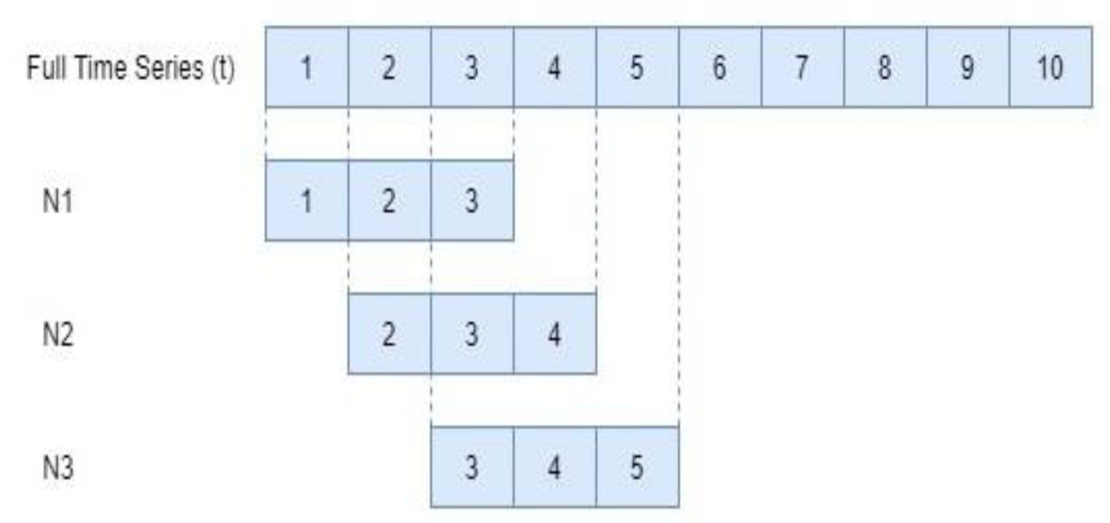
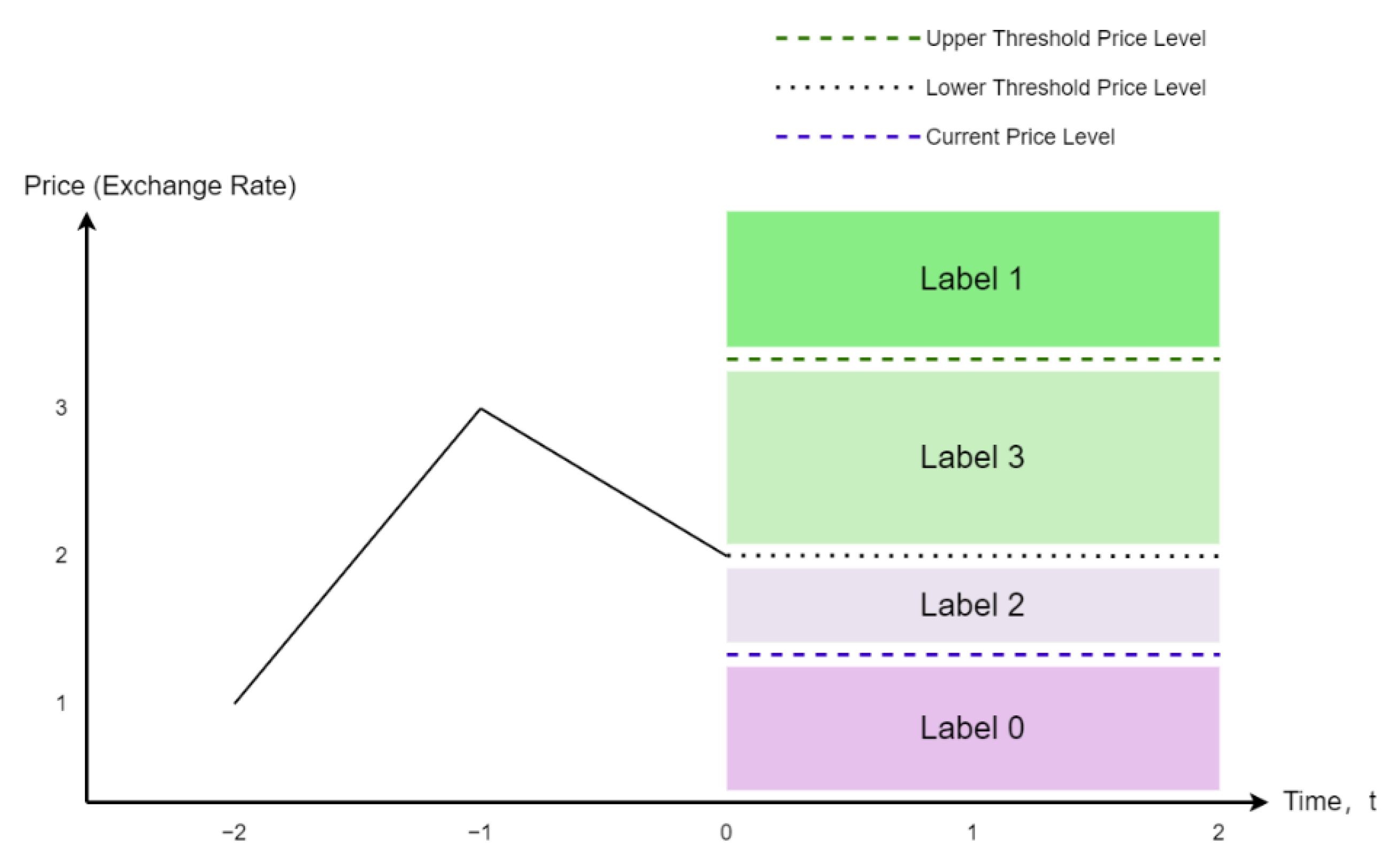
3.3. Data Generation
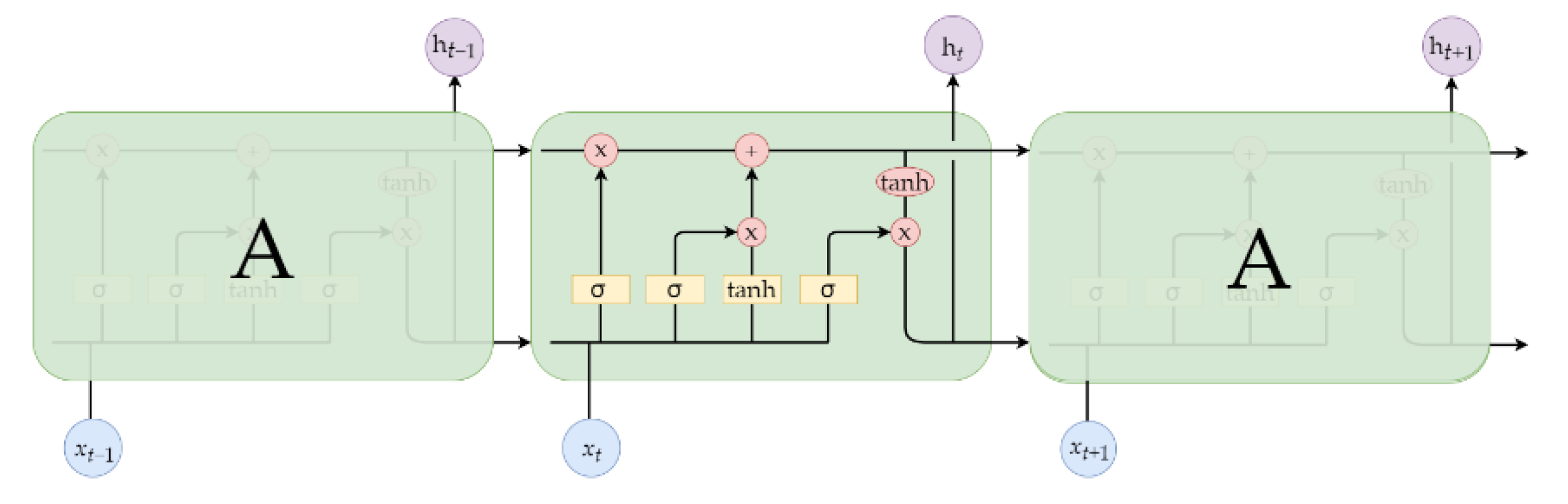
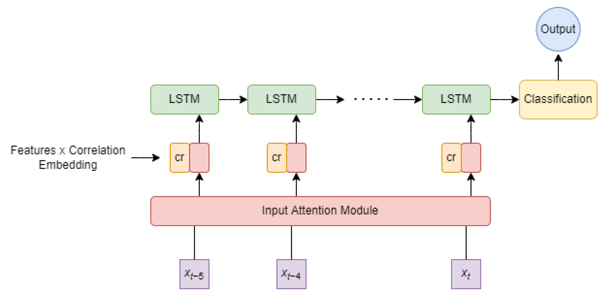
3.4. Model Framework
4. Performance Results
5. Conclusions
Author Contributions
Funding
Institutional Review Board Statement
Informed Consent Statement
Conflicts of Interest
References
- Treleaven, P.; Galas, M.; Lalchand, V. Algorithmic trading review. Commun. ACM 2013, 56, 76–85. [Google Scholar] [CrossRef]
- Daoud, J.I. Multicollinearity and Regression Analysis. J. Phys. Conf. Ser. 2017, 949, 012009. [Google Scholar] [CrossRef]
- Bollinger, J. Using bollinger bands. Stock. Commod. 1992, 10, 47–51. [Google Scholar]
- Khaire, U.M.; Dhanalakshmi, R. Stability of feature selection algorithm: A review. J. King Saud Univ.-Comput. Inf. Sci. 2019, 34, 1060–1073. [Google Scholar] [CrossRef]
- Obite, C.P.; Olewuezi, N.P.; Ugwuanyim, G.U.; Bartholomew, D.C. Multicollinearity Effect in Regression Analysis: A Feed forward Artificial Neural Network Approach. Asian J. Probab. Stat. 2020, 6, 22–33. [Google Scholar] [CrossRef]
- Wu, Y.-C.; Feng, J.-W. Development and Application of Artificial Neural Network. Wirel. Pers. Commun. 2018, 102, 1645–1656. [Google Scholar] [CrossRef]
- Lucey, B.M.; Muckley, C. Robust global stock market interdependencies. Int. Rev. Financ. Anal. 2011, 20, 215–224. [Google Scholar] [CrossRef]
- Bahdanau, D.; Cho, K.; Bengio, Y. Neural Machine Translation by Jointly Learning to Align and Translate. arXiv 2014, arXiv:1409.0473. [Google Scholar]
- Yuan, H.; Zhou, H.; Cai, Z.; Zhang, S.; Wu, R. Dynamic Pyramid Attention Networks for multi-orientation object detection. J. Internet Tech. 2022, 23, 79–90. [Google Scholar]
- Lee, M.-C. Research on the Feasibility of Applying GRU and Attention Mechanism Combined with Technical Indicators in Stock Trading Strategies. Appl. Sci. 2022, 12, 1007. [Google Scholar] [CrossRef]
- Siami-Namini, S.; Namin, A.S. Forecasting economics and financial time series: ARIMA vs. LSTM. arXiv 2018, arXiv:180306386. [Google Scholar]
- M’ng, J.C.P.; Aziz, A.A. Using neural networks to enhance technical trading rule returns: A case with KLCI. Athens J. Bus. Econ. 2016, 2, 63–70. [Google Scholar] [CrossRef]
- Rundo, F. Deep LSTM with Reinforcement Learning Layer for Financial Trend Prediction in FX High Frequency Trading Systems. Appl. Sci. 2019, 9, 4460. [Google Scholar] [CrossRef]
- Katrutsa, A.; Strijov, V. Comprehensive study of feature selection methods to solve multicollinearity problem according to evaluation criteria. Expert Syst. Appl. 2017, 76, 1–11. [Google Scholar] [CrossRef]
- Smith, G. Step away from stepwise. J. Big Data 2018, 5, 32. [Google Scholar] [CrossRef]
- Horel, A. Applications of ridge analysis to regression problems. Chem. Eng. Prog. 1962, 58, 54–59. [Google Scholar]
- Nguyen, V.C.; Ng, C.T. Variable selection under multicollinearity using modified log penalty. J. Appl. Stat. 2019, 47, 201–230. [Google Scholar] [CrossRef]
- Garg, A.; Tai, K. Comparison of regression analysis, artificial neural network and genetic programming in handling the multicollinearity problem. In Proceedings of the 2012 International Conference on Modelling, Identifi-Cation and Control, IEEE, Wuhan, China, 24–26 June 2012; pp. 353–358. [Google Scholar]
- Rasekhschaffe, K.C.; Jones, R.C. Machine Learning for Stock Selection. Financ. Anal. J. 2019, 75, 70–88. [Google Scholar] [CrossRef]
- Huynh, H.; Won, Y. Regularized online sequential learning algorithm for single-hidden layer feedforward neural networks. Pattern Recognit. Lett. 2011, 32, 1930–1935. [Google Scholar] [CrossRef]
- Guo, L.; Hao, J.-H.; Liu, M. An incremental extreme learning machine for online sequential learning problems. Neurocomputing 2014, 128, 50–58. [Google Scholar] [CrossRef]
- Nóbrega, J.P.; Oliveira, A.L. A sequential learning method with Kalman filter and extreme learning machine for regression and time series forecasting. Neurocomputing 2019, 337, 235–250. [Google Scholar] [CrossRef]
- Tamura, R.; Kobayashi, K.; Takano, Y.; Miyashiro, R.; Nakata, K.; Matsui, T. Best subset selection for eliminating multicollinearity. J. Oper. Res. Soc. Jpn. 2017, 60, 321–336. [Google Scholar] [CrossRef][Green Version]
- Sezer, O.B.; Ozbayoglu, A.M.; Dogdu, E. An artificial neural network-based stock trading system using tech-nical analysis and big data framework. In Proceedings of the Southeast Conference ACMSE, Kennesaw, GA, USA, 13–15 April 2017. [Google Scholar]
- Nuti, G.; Mirghaemi, M.; Treleaven, P.; Yingsaeree, C. Algorithmic trading. Computer 2011, 44, 61–69. [Google Scholar] [CrossRef]
- Krishnaveni, P.; Swarnam, S.; Prabakaran, V. An empirical study to analyse overbought and oversold periods of shares listed in CNX Bankex. Int. J. Manag. 2019, 9, 155–167. [Google Scholar]
- Lavery, M.R.; Acharya, P.; Sivo, S.A.; Xu, L. Number of predictors and multicollinearity: What are their effects on error and bias in regression? Commun. Stat.-Simul. Comput. 2017, 48, 27–38. [Google Scholar] [CrossRef]
- Althelaya, K.A.; El-Alfy, E.-S.M.; Mohammed, S. Evaluation of bidirectional LSTM for short-and long-term stock market prediction. In Proceedings of the 2018 9th International Conference on Information and Communication Systems, Irbid, Jordan, 3–5 April 2018; pp. 151–156. [Google Scholar]


| Variables | VIF |
|---|---|
| open | 20,637 |
| high | 17,431 |
| low | 20,848 |
| close | 24,950 |
| RSI | 7 |
| MACD | 21 |
| SAR | 877 |
| SMA 5 | 13,692 |
| SMA 10 | 3599 |
| SMA 20 | 243,345 |
| CMA | 4 |
| EMA | 67,907 |
| %K | 32 |
| %D | 13 |
| %R | 19 |
| Bollinger High | 61,274 |
| Bollinger Low | 62,111 |
| Evaluation Metric | LSTM | MRM LSTM |
|---|---|---|
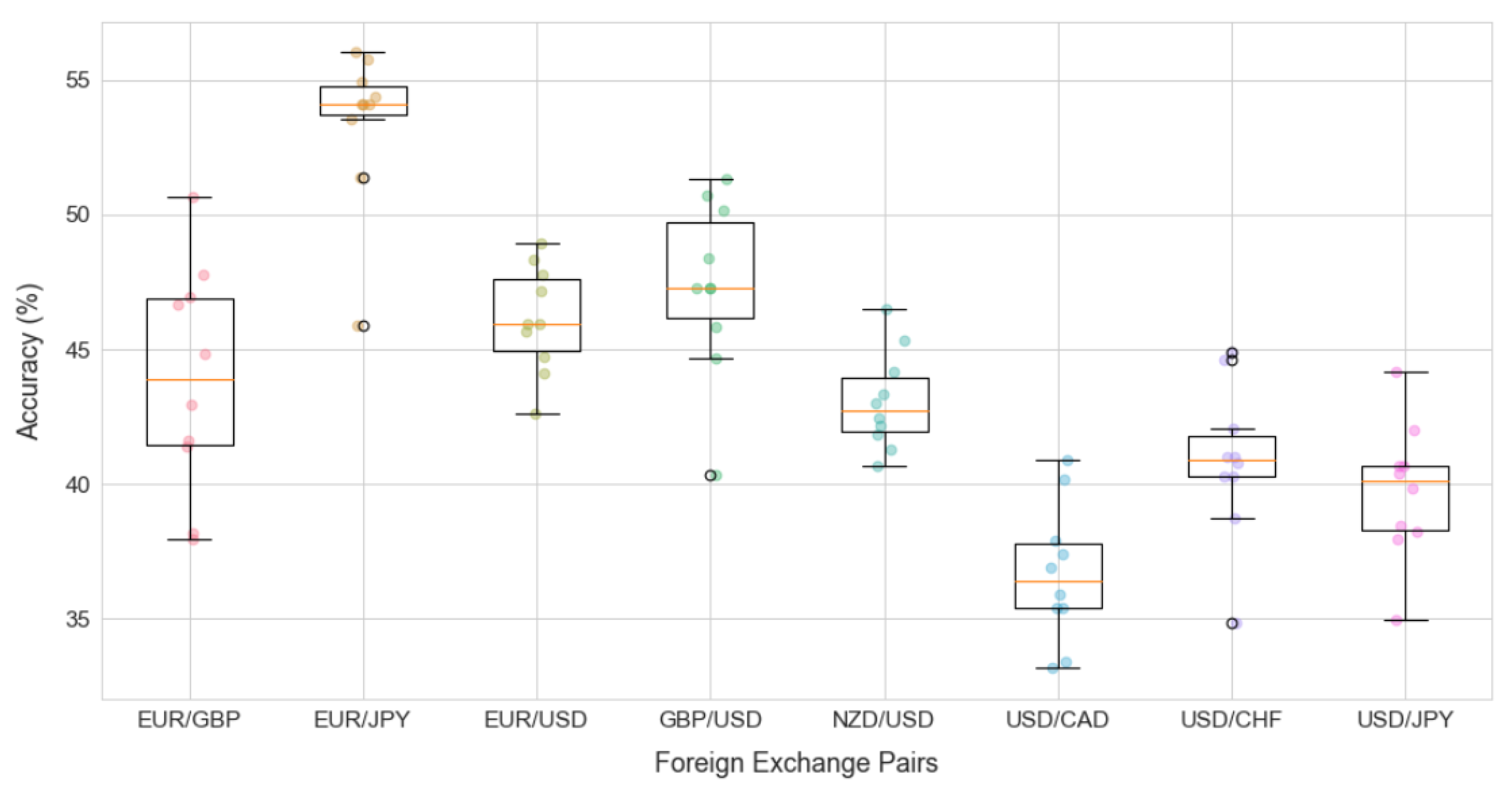
| Mean of Accuracy | 45.43% | 43.88% |
| Std of Accuracy | 2.54% | 2.62% |
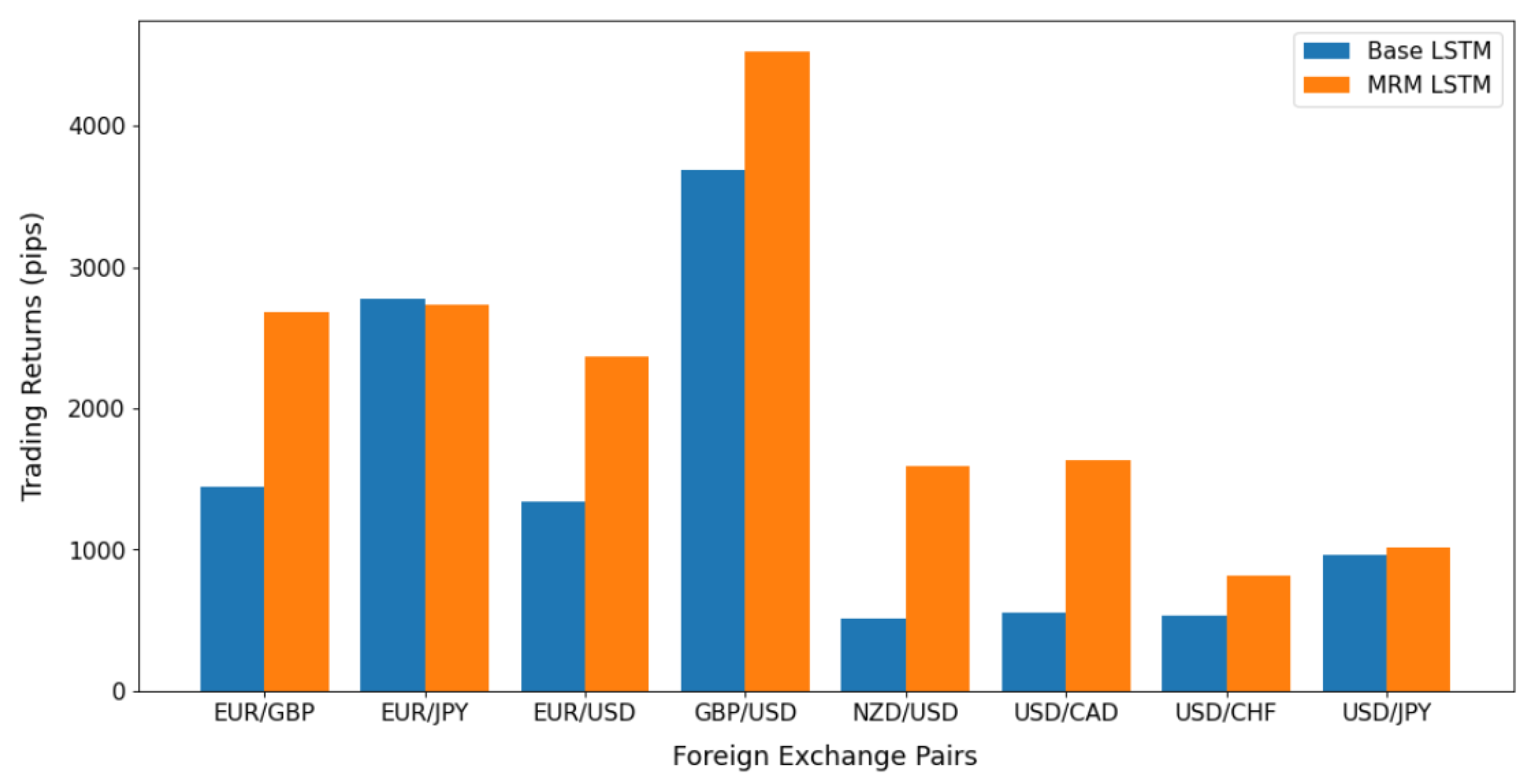
| Mean of Returns (pips) | 1476.14 | 2167.34 |
| Std of Returns (pips) | 452.01 | 525.88 |
| Mean of Loss Function | 0.8435 | 0.5088 |
| Std of Loss Function | 0.0241 | 0.0750 |
Publisher’s Note: MDPI stays neutral with regard to jurisdictional claims in published maps and institutional affiliations. |
© 2022 by the authors. Licensee MDPI, Basel, Switzerland. This article is an open access article distributed under the terms and conditions of the Creative Commons Attribution (CC BY) license (https://creativecommons.org/licenses/by/4.0/).
Share and Cite
Chan, J.Y.-L.; Leow, S.M.H.; Bea, K.T.; Cheng, W.K.; Phoong, S.W.; Hong, Z.-W.; Lin, J.-M.; Chen, Y.-L. A Correlation-Embedded Attention Module to Mitigate Multicollinearity: An Algorithmic Trading Application. Mathematics 2022, 10, 1231. https://doi.org/10.3390/math10081231
Chan JY-L, Leow SMH, Bea KT, Cheng WK, Phoong SW, Hong Z-W, Lin J-M, Chen Y-L. A Correlation-Embedded Attention Module to Mitigate Multicollinearity: An Algorithmic Trading Application. Mathematics. 2022; 10(8):1231. https://doi.org/10.3390/math10081231
Chicago/Turabian StyleChan, Jireh Yi-Le, Steven Mun Hong Leow, Khean Thye Bea, Wai Khuen Cheng, Seuk Wai Phoong, Zeng-Wei Hong, Jim-Min Lin, and Yen-Lin Chen. 2022. "A Correlation-Embedded Attention Module to Mitigate Multicollinearity: An Algorithmic Trading Application" Mathematics 10, no. 8: 1231. https://doi.org/10.3390/math10081231
APA StyleChan, J. Y.-L., Leow, S. M. H., Bea, K. T., Cheng, W. K., Phoong, S. W., Hong, Z.-W., Lin, J.-M., & Chen, Y.-L. (2022). A Correlation-Embedded Attention Module to Mitigate Multicollinearity: An Algorithmic Trading Application. Mathematics, 10(8), 1231. https://doi.org/10.3390/math10081231