
A Stepwise Algorithm for Linearly Combining Biomarkers under Youden Index Maximization

 ,
,  , , and
Abstract
:1. Introduction
2. Materials and Methods
2.1. Background: Non Parametric Approach
2.2. Our Proposed Stepwise Approach
- Firstly, given p biomarkers, the linear combination of the two biomarkers that maximizes the Youden index is chosen,using empirical search proposed by Pepe et al.: for each biomarker pair, for each value of the 201 , the optimal cut-off point that maximizes Youden index is selected. The final value chosen is the one with the highest Youden obtained;
- Once the pair of biomarkers and the parameter that maximizes the Youden index are chosen, this linear combination is considered as a single variable. For simplicity, suppose the linear combination . Then, in the same way as point 1, the biomarker (of the remaining s) and the parameter whose new linear combination maximize the Youden index are selected:Specifically, either the combination (7) or (8) that maximizes the Youden index is selected. This new linear combination will be considered as a new variable in the next step;
- The process (2) is repeated for the rest of biomarkers (i.e., times) until all of them are included in the model.
2.3. Yin and Tian’s Stepwise Approach
2.4. Min-Max Approach
2.5. Logistic Regression
2.6. Parametric Approach under Multivariate Normality
2.7. Non-Parametric Kernel Smoothing Approach
2.8. Simulations
2.9. Application in Clinical Diagnosis Cases
2.10. Validation
3. Results
3.1. Simulations
3.1.1. Normal Distributions. Different Means and Equal Positive Correlations for Diseased and Non-Diseased Population

| Mean (SD) | Probability Greater than or Equal to Youden Index | ||||||||||||
|---|---|---|---|---|---|---|---|---|---|---|---|---|---|
| Size (, ) | Mean (SD) Variables | SLM | SWD | MM | LR | MVN | KS | SLM | SWD | MM | LR | MVN | KS |
| (10, 20) | = (0.2737, 0.3560, 0.5178, 0.4314) | 0.7782 | 0.731 | 0.6352 | 0.6926 | 0.6937 | 0.7272 | 0.5962 | 0.1389 | 0.0588 | 0.0532 | 0.0355 | 0.1175 |
| = (0.1357, 0.1395, 0.1421, 0.1457) | (0.1022) | (0.1104) | (0.119) | (0.1346) | (0.1253) | (0.1179) | |||||||
| (30, 30) | = (0.2063, 0.3024, 0.4663, 0.3673) | 0.6737 | 0.6402 | 0.5556 | 0.6057 | 0.6050 | 0.6395 | 0.6480 | 0.1350 | 0.0453 | 0.0221 | 0.0161 | 0.1335 |
| = (0.0943, 0.0991, 0.0990, 0.1053) | (0.0836) | (0.0876) | (0.0962) | (0.0957) | (0.0946) | (0.0891) | |||||||
| (50, 30) | = (0.1933, 0.2975, 0.4630, 0.3603) | 0.6434 | 0.6278 | 0.5424 | 0.5895 | 0.5896 | 0.6203 | 0.5806 | 0.1756 | 0.0448 | 0.0179 | 0.0176 | 0.1636 |
| = (0.0846, 0.0937, 0.0894, 0.0898) | (0.0771) | (0.0778) | (0.0812) | (0.0839) | (0.0828) | (0.0806) | |||||||
| (50, 50) | = (0.1764, 0.2784, 0.4484, 0.3458) | 0.6219 | 0.6005 | 0.5193 | 0.5693 | 0.5693 | 0.5998 | 0.6586 | 0.1428 | 0.0272 | <0.01 | 0.0132 | 0.1495 |
| = (0.0736, 0.0789, 0.0774, 0.0796) | (0.0667) | (0.0702) | (0.0736) | (0.0732) | (0.0732) | (0.0701) | |||||||
| (100, 100) | = (0.1487, 0.2498, 0.4254, 0.3214) | 0.5734 | 0.5623 | 0.4837 | 0.5412 | 0.5409 | 0.5620 | 0.6174 | 0.1543 | 0.0132 | 0.0171 | 0.0137 | 0.1844 |
| = (0.0533, 0.0590, 0.0560, 0.0590) | (0.0506) | (0.051) | (0.0526) | (0.0538) | (0.0537) | (0.0528) | |||||||
| (500, 500) | = (0.1062, 0.2185, 0.3991, 0.2925) | 0.5213 | 0.5191 | 0.4447 | 0.5120 | 0.5119 | 0.5196 | 0.4545 | 0.1824 | <0.01 | 0.0332 | 0.0317 | 0.2982 |
| = (0.0257, 0.0282, 0.0274, 0.0280) | (0.0257) | (0.0257) | (0.027) | (0.0262) | (0.0263) | (0.0258) | |||||||
| (10, 20) | = (0.3359, 0.5120, 0.6604, 0.5815) | 0.9134 | 0.8783 | 0.8042 | 0.8771 | 0.8594 | 0.8786 | 0.4822 | 0.1128 | 0.0350 | 0.1913 | 0.0565 | 0.1221 |
| = (0.1413, 0.1386, 0.1275, 0.1402) | (0.074) | (0.0834) | (0.1013) | (0.0158) | (0.0958) | (0.0886) | |||||||
| (30, 30) | = (0.2699, 0.4695, 0.6172, 0.5299) | 0.8488 | 0.8190 | 0.7463 | 0.8086 | 0.8044 | 0.8242 | 0.5826 | 0.1304 | 0.0319 | 0.0692 | 0.0420 | 0.1438 |
| = (0.0989, 0.0988, 0.0911, 0.1019) | (0.0645) | (0.0690) | (0.0787) | (0.0778) | (0.0750) | (0.0719) | |||||||
| (50, 30) | = (0.2586, 0.4636, 0.6133, 0.5218) | 0.8310 | 0.8172 | 0.7400 | 0.8005 | 0.7960 | 0.8162 | 0.5270 | 0.1755 | 0.0372 | 0.0540 | 0.0362 | 0.1700 |
| = (0.0905, 0.0926, 0.0810, 0.0854) | (0.0598) | (0.0621) | (0.069) | (0.0676) | (0.0666) | (0.0633) | |||||||
| (50, 50) | = (0.2444, 0.4475, 0.6010, 0.5099) | 0.8144 | 0.7972 | 0.7235 | 0.7840 | 0.7806 | 0.8007 | 0.5841 | 0.1403 | 0.0199 | 0.0436 | 0.0295 | 0.1826 |
| = (0.0791, 0.0796, 0.0695, 0.0772) | (0.0545) | (0.0569) | (0.0624) | (0.0598) | (0.0584) | (0.0573) | |||||||
| (100, 100) | = (0.2178, 0.4243, 0.5821, 0.4906) | 0.7827 | 0.7728 | 0.6987 | 0.7620 | 0.7611 | 0.7749 | 0.5701 | 0.1690 | <0.01 | 0.0262 | 0.0286 | 0.2036 |
| = (0.0570, 0.0579, 0.0526, 0.0562) | (0.04) | (0.0412) | (0.0456) | (0.0423) | (0.0423) | (0.0412) | |||||||
| (500, 500) | = (0.1809, 0.3997, 0.5604, 0.4673) | 0.7483 | 0.7461 | 0.6692 | 0.7424 | 0.7422 | 0.7471 | 0.4667 | 0.1695 | <0.01 | 0.0431 | 0.0359 | 0.2848 |
| = (0.0271, 0.0272, 0.0255, 0.0260) | (0.02) | (0.0199) | (0.0223) | (0.0201) | (0.0201) | (0.0199) | |||||||
| Mean (SD) | Probability Greater than or Equal to Youden Index | ||||||||||||
|---|---|---|---|---|---|---|---|---|---|---|---|---|---|
| Size (, ) | Mean (SD) Variables | SLM | SWD | MM | LR | MVN | KS | SLM | SWD | MM | LR | MVN | KS |
| (10, 20) | = (0.2666, 0.3621, 0.5180, 0.4226) | 0.7348 | 0.6811 | 0.5730 | 0.6380 | 0.6385 | 0.6755 | 0.6163 | 0.1309 | 0.0617 | 0.0404 | 0.0312 | 0.1195 |
| = (0.1378, 0.1439, 0.1377, 0.1427) | (0.1063) | (0.1158) | (0.1294) | (0.1389) | (0.1358) | (0.1266) | |||||||
| (30, 30) | = (0.2037, 0.3051, 0.4700, 0.3774) | 0.6228 | 0.5873 | 0.4842 | 0.5472 | 0.5483 | 0.5844 | 0.6869 | 0.1276 | 0.0343 | 0.0103 | 0.0125 | 0.1284 |
| = (0.0951, 0.1029, 0.1002, 0.1004) | (0.0848) | (0.0896) | (0.0948) | (0.0994) | (0.0982) | (0.0939) | |||||||
| (50, 30) | = (0.1963,0.2917,0.4606,0.3620) | 0.5905 | 0.5701 | 0.4677 | 0.5278 | 0.5284 | 0.5628 | 0.6378 | 0.1491 | 0.0322 | 0.0151 | 0.0141 | 0.1517 |
| = (0.0841, 0.0888, 0.0899, 0.0903) | (0.0788) | (0.0787) | (0.0831) | (0.0868) | (0.0862) | (0.0852) | |||||||
| (50, 50) | = (0.1771, 0.2780, 0.4448, 0.3459) | 0.5641 | 0.5380 | 0.4435 | 0.5030 | 0.5038 | 0.5354 | 0.7324 | 0.1176 | 0.0165 | 0.0123 | 0.0113 | 0.1098 |
| = (0.0751, 0.0798, 0.0778, 0.0805) | (0.0683) | (0.0707) | (0.0753) | (0.0752) | (0.0756) | (0.0717) | |||||||
| (100, 100) | = (0.1464, 0.2526, 0.4270, 0.3230) | 0.5148 | 0.5012 | 0.4078 | 0.4770 | 0.4768 | 0.4984 | 0.6986 | 0.1268 | <0.01 | 0.013 | <0.01 | 0.1457 |
| = (0.0515, 0.0593, 0.0580, 0.0591) | (0.0546) | (0.0550) | (0.0542) | (0.0584) | (0.0585) | (0.0563) | |||||||
| (500, 500) | = (0.1063, 0.2178, 0.3980, 0.2923) | 0.4524 | 0.449 | 0.3586 | 0.4404 | 0.4402 | 0.4488 | 0.5629 | 0.1693 | <0.01 | 0.0234 | 0.0222 | 0.2221 |
| = (0.0262, 0.0282, 0.0278, 0.0278) | (0.0264) | (0.0265) | (0.0271) | (0.0269) | (0.0268) | (0.0265) | |||||||
| (10, 20) | = (0.3272, 0.5176, 0.6594, 0.5757) | 0.8558 | 0.8128 | 0.7198 | 0.7941 | 0.7847 | 0.809 | 0.5515 | 0.1334 | 0.0565 | 0.1059 | 0.0445 | 0.1081 |
| = (0.1436, 0.1440, 0.1291, 0.1388) | (0.0907) | (0.1001) | (0.1174) | (0.1256) | (0.1137) | (0.1056) | |||||||
| (30, 30) | = (0.2685, 0.4690, 0.6182, 0.5362) | 0.7751 | 0.7433 | 0.6514 | 0.7196 | 0.7175 | 0.7433 | 0.6647 | 0.1203 | 0.0238 | 0.0329 | 0.0271 | 0.1313 |
| = (0.1006, 0.1013, 0.0920, 0.0949) | (0.0742) | (0.0772) | (0.0892) | (0.0852) | (0.0841) | (0.082) | |||||||
| (50,30) | = (0.2629, 0.4602, 0.6113, 0.5246) | 0.7515 | 0.7343 | 0.6393 | 0.7057 | 0.7047 | 0.7291 | 0.643 | 0.1586 | 0.0228 | 0.0243 | 0.0204 | 0.1308 |
| = (0.0891, 0.0909, 0.0813, 0.0870) | (0.0681) | (0.0705) | (0.078) | (0.0779) | (0.0762) | (0.0733) | |||||||
| (50, 50) | = (0.2441, 0.4483, 0.5975, 0.5108) | 0.7307 | 0.7107 | 0.6204 | 0.6883 | 0.6870 | 0.7109 | 0.6652 | 0.1333 | 0.0168 | 0.0217 | 0.021 | 0.142 |
| = (0.0793, 0.0795, 0.0729, 0.0761) | (0.0609) | (0.0646) | (0.0702) | (0.0675) | (0.0673) | (0.0648) | |||||||
| (100, 100) | = (0.2160, 0.4258, 0.5829, 0.4909) | 0.6934 | 0.6818 | 0.5922 | 0.6642 | 0.6641 | 0.6814 | 0.655 | 0.1473 | <0.01 | 0.0229 | 0.0229 | 0.1485 |
| = (0.0537, 0.0578, 0.0529, 0.0567) | (0.0488) | (0.0488) | (0.0496) | (0.0525) | (0.0516) | (0.0492) | |||||||
| (500, 500) | = (0.1803, 0.3987, 0.5594, 0.4663) | 0.6453 | 0.643 | 0.5543 | 0.6379 | 0.6378 | 0.6436 | 0.4826 | 0.1741 | <0.01 | 0.0363 | 0.0354 | 0.2717 |
| = (0.0277, 0.0274, 0.0252, 0.0266) | (0.023) | (0.023) | (0.0244) | (0.0237) | (0.0238) | (0.0229) | |||||||
| Mean (SD) | Probability Greater than or Equal to Youden Index | ||||||||||||
|---|---|---|---|---|---|---|---|---|---|---|---|---|---|
| Size (, ) | Mean (SD) Variables | SLM | SWD | MM | LR | MVN | KS | SLM | SWD | MM | LR | MVN | KS |
| (10, 20) | = (0.2713, 0.3657, 0.5268, 0.428) | 0.7314 | 0.667 | 0.5534 | 0.6404 | 0.6432 | 0.674 | 0.4883 | 0.1566 | 0.0399 | 0.0496 | 0.0804 | 0.1851 |
| = (0.1353, 0.1477, 0.1423, 0.1427) | (0.1093) | (0.1181) | (0.1271) | (0.1387) | (0.1356) | (0.1306) | |||||||
| (30, 30) | = (0.2030, 0.3020, 0.4665, 0.3668) | 0.62 | 0.5647 | 0.4598 | 0.548 | 0.5433 | 0.5777 | 0.5478 | 0.1417 | 0.0118 | 0.0244 | 0.0572 | 0.2171 |
| = (0.0933, 0.1014, 0.0991, 0.1008) | (0.0847) | (0.0882) | (0.0945) | (0.0972) | (0.0952) | (0.0921) | |||||||
| (50, 30) | = (0.1931, 0.2928, 0.4581, 0.3632) | 0.5874 | 0.5568 | 0.4415 | 0.5288 | 0.5297 | 0.5631 | 0.4942 | 0.1885 | <0.01 | 0.0295 | 0.0282 | 0.2543 |
| = (0.0847, 0.0908, 0.0883, 0.0905) | (0.0769) | (0.0764) | (0.0811) | (0.0856) | (0.0842) | (0.0831) | |||||||
| (50, 50) | = (0.1753, 0.2761, 0.4472, 0.3495) | 0.5637 | 0.5274 | 0.4187 | 0.5096 | 0.5094 | 0.5401 | 0.5076 | 0.1588 | <0.01 | 0.0247 | 0.0502 | 0.2528 |
| = (0.0742, 0.0798, 0.0787, 0.0791) | (0.0677) | (0.0717) | (0.0738) | (0.0755) | (0.0746) | (0.0738) | |||||||
| (100, 100) | = (0.1449, 0.2487, 0.4250, 0.3236) | 0.5114 | 0.4907 | 0.3806 | 0.4766 | 0.4766 | 0.5005 | 0.4238 | 0.3977 | <0.01 | 0.0152 | <0.01 | 0.1548 |
| = (0.0520, 0.0578, 0.0591, 0.0595) | (0.0539) | (0.0551) | (0.056) | (0.0583) | (0.0584) | (0.0566) | |||||||
| (500, 500) | = (0.1063, 0.2187, 0.3994, 0.2921) | 0.4511 | 0.443 | 0.3325 | 0.4429 | 0.4429 | 0.4516 | 0.3103 | 0.3948 | <0.01 | 0.0237 | 0.0204 | 0.2508 |
| = (0.0261, 0.0280, 0.0264, 0.0279) | (0.0256) | (0.0276) | (0.0272) | (0.0265) | (0.0265) | (0.0256) | |||||||
| (10, 20) | = (0.3339, 0.5172, 0.6658, 0.5790) | 0.844 | 0.7906 | 0.6879 | 0.7838 | 0.7736 | 0.7996 | 0.4078 | 0.1614 | 0.0258 | 0.1348 | 0.0884 | 0.1817 |
| = (0.1406, 0.1442, 0.1287, 0.1370) | (0.0934) | (0.1050) | (0.1184) | (0.1288) | (0.1167) | (0.1107) | |||||||
| (30, 30) | = (0.2685, 0.4669, 0.6160, 0.5254) | 0.7609 | 0.7139 | 0.6157 | 0.7084 | 0.7007 | 0.7294 | 0.5169 | 0.1461 | 0.0115 | 0.0512 | 0.0628 | 0.2116 |
| = (0.0998, 0.1025, 0.0945, 0.0954) | (0.0766) | (0.0801) | (0.0906) | (0.0876) | (0.087) | (0.0804) | |||||||
| (50, 30) | = (0.2580, 0.4621, 0.6105, 0.5264) | 0.7348 | 0.7101 | 0.6034 | 0.6945 | 0.6929 | 0.7177 | 0.4785 | 0.1823 | <0.01 | 0.0643 | 0.0438 | 0.2257 |
| = (0.0887, 0.0908, 0.0807, 0.0862) | (0.0686) | (0.0707) | (0.0782) | (0.0773) | (0.0743) | (0.0721) | |||||||
| (50, 50) | = (0.2428, 0.4477, 0.5994, 0.5124) | 0.7162 | 0.6874 | 0.5831 | 0.6778 | 0.6762 | 0.7013 | 0.4817 | 0.1485 | <0.01 | 0.0496 | 0.0575 | 0.2574 |
| = (0.0782, 0.0810, 0.0723, 0.0769) | (0.0620) | (0.0649) | (0.0715) | (0.0697) | (0.0665) | (0.0639) | |||||||
| (100, 100) | = (0.2146, 0.4235, 0.5816, 0.4916) | 0.6755 | 0.6572 | 0.5535 | 0.6519 | 0.6513 | 0.6684 | 0.5904 | 0.083 | <0.01 | 0.04 | 0.0382 | 0.2475 |
| = (0.0554, 0.0572, 0.0550, 0.0580) | (0.0480) | (0.0493) | (0.0524) | (0.0510) | (0.0509) | (0.0494) | |||||||
| (500, 500) | = (0.1808, 0.3990, 0.5606, 0.4663) | 0.6286 | 0.6239 | 0.5165 | 0.6258 | 0.6255 | 0.6317 | 0.379 | 0.1055 | <0.01 | 0.0561 | 0.0563 | 0.403 |
| = (0.0270, 0.0277, 0.0244, 0.0260) | (0.0236) | (0.0242) | (0.0251) | (0.0232) | (0.0232) | (0.023) | |||||||
| Mean (SD) | Probability Greater than or Equal to Youden Index | ||||||||||||
|---|---|---|---|---|---|---|---|---|---|---|---|---|---|
| Size (, ) | Mean (SD) Variables | SLM | SWD | MM | LR | MVN | KS | SLM | SWD | MM | LR | MVN | KS |
| (10, 20) | = (0.2708, 0.3672, 0.5202, 0.4299) | 0.754 | 0.6634 | 0.5546 | 0.6702 | 0.6704 | 0.6962 | 0.5549 | 0.1035 | 0.0211 | 0.0879 | 0.0684 | 0.1642 |
| = (0.1361, 0.1398, 0.1435, 0.1447) | (0.1036) | (0.119) | (0.1268) | (0.1418) | (0.1383) | (0.1317) | |||||||
| (30, 30) | = (0.2005, 0.3040, 0.4663, 0.3703) | 0.6514 | 0.5668 | 0.4559 | 0.5844 | 0.5834 | 0.6166 | 0.5812 | 0.0826 | 0.0116 | 0.0521 | 0.0397 | 0.2329 |
| = (0.0936, 0.1025, 0.1045, 0.1038) | (0.0817) | (0.0937) | (0.0946) | (0.0981) | (0.0972) | (0.0940) | |||||||
| (50, 30) | = (0.1951, 0.2932, 0.4625, 0.3591) | 0.6175 | 0.5628 | 0.4401 | 0.5689 | 0.5690 | 0.6000 | 0.5288 | 0.1146 | <0.01 | 0.0414 | 0.0324 | 0.2768 |
| = (0.0815, 0.0877, 0.0893, 0.0914) | (0.0779) | (0.0834) | (0.0817) | (0.0882) | (0.0874) | (0.0859) | |||||||
| (50, 50) | = (0.1781, 0.2779, 0.4479, 0.3450) | 0.5983 | 0.5325 | 0.4166 | 0.5527 | 0.5521 | 0.5805 | 0.5430 | 0.0799 | <0.01 | 0.0454 | 0.0431 | 0.2858 |
| = (0.0735, 0.0787, 0.0800, 0.0806) | (0.0671) | (0.0754) | (0.0747) | (0.0782) | (0.0774) | (0.0741) | |||||||
| (100, 100) | = (0.1461, 0.2526, 0.4243, 0.3207) | 0.5472 | 0.4969 | 0.3773 | 0.5203 | 0.5202 | 0.5413 | 0.4680 | 0.2348 | <0.01 | 0.0173 | 0.0222 | 0.2577 |
| = (0.0534, 0.0597, 0.0566, 0.0606) | (0.0515) | (0.0567) | (0.0548) | (0.0547) | (0.0547) | (0.0530) | |||||||
| (500, 500) | = (0.1057, 0.2177, 0.3992, 0.2928) | 0.4949 | 0.4587 | 0.3313 | 0.4893 | 0.4892 | 0.4972 | 0.3588 | 0.1517 | <0.01 | 0.0418 | 0.0358 | 0.4118 |
| = (0.0267, 0.0281, 0.0276, 0.0278) | (0.0257) | (0.0308) | (0.0274) | (0.0260) | (0.0259) | (0.0255) | |||||||
| (10, 20) | = (0.3322, 0.5204, 0.6594, 0.5826) | 0.8612 | 0.7759 | 0.6874 | 0.8091 | 0.7979 | 0.8204 | 0.5229 | 0.0699 | 0.0183 | 0.1656 | 0.0730 | 0.1503 |
| = (0.1426, 0.1414, 0.1301, 0.1402) | (0.0882) | (0.1107) | (0.1232) | (0.1266) | (0.1156) | (0.1099) | |||||||
| (30, 30) | = (0.2669, 0.4678, 0.6169, 0.5312) | 0.7842 | 0.7095 | 0.6146 | 0.7393 | 0.7369 | 0.7607 | 0.5373 | 0.0759 | <0.01 | 0.0856 | 0.0629 | 0.2325 |
| = (0.0982, 0.0999, 0.0961, 0.1011) | (0.0702) | (0.0854) | (0.0884) | (0.0835) | (0.0821) | (0.0782) | |||||||
| (50,30) | = (0.2620, 0.4584, 0.6136, 0.5234) | 0.7596 | 0.7128 | 0.6007 | 0.7304 | 0.7283 | 0.7514 | 0.4932 | 0.0898 | <0.01 | 0.0842 | 0.0564 | 0.2714 |
| = (0.0865, 0.0865, 0.0817, 0.0866) | (0.0682) | (0.0722) | (0.078) | (0.0760) | (0.0735) | (0.0696) | |||||||
| (50, 50) | = (0.2458, 0.4465, 0.6006, 0.5098) | 0.7394 | 0.6899 | 0.5806 | 0.7165 | 0.7149 | 0.7361 | 0.4764 | 0.0643 | <0.01 | 0.0650 | 0.0637 | 0.3282 |
| = (0.0776, 0.0776, 0.0756, 0.0769) | (0.0612) | (0.0717) | (0.0729) | (0.0676) | (0.0663) | (0.0638) | |||||||
| (100, 100) | = (0.2155, 0.4256, 0.5809, 0.4890) | 0.7018 | 0.6658 | 0.5523 | 0.6898 | 0.6886 | 0.7036 | 0.4592 | 0.0528 | <0.01 | 0.0712 | 0.0544 | 0.3625 |
| = (0.0562, 0.0606, 0.0520, 0.0570) | (0.042) | (0.0525) | (0.0502) | (0.0469) | (0.047) | (0.0458) | |||||||
| (500, 500) | = (0.1802, 0.3992, 0.5603, 0.4668) | 0.6588 | 0.6451 | 0.5148 | 0.6643 | 0.6643 | 0.6701 | 0.1175 | 0.2240 | <0.01 | 0.0793 | 0.0653 | 0.5138 |
| = (0.0280, 0.0267, 0.0250, 0.0256) | (0.0226) | (0.0270) | (0.0253) | (0.0222) | (0.0222) | (0.0220) | |||||||
3.1.2. Normal Distributions. Different Means and Unequal Positive Correlations for Diseased and Non-Diseased Population
| Mean (SD) | Probability Greater than or Equal to Youden Index | ||||||||||||
|---|---|---|---|---|---|---|---|---|---|---|---|---|---|
| Size (, ) | Mean (SD) Variables | SLM | SWD | MM | LR | MVN | KS | SLM | SWD | MM | LR | MVN | KS |
| (10, 20) | = (0.2706, 0.3608, 0.5172, 0.4272) | 0.736 | 0.6644 | 0.5952 | 0.637 | 0.6408 | 0.669 | 0.4899 | 0.1413 | 0.0987 | 0.0536 | 0.0679 | 0.1486 |
| = (0.1367, 0.1405, 0.1453, 0.1456) | (0.0998) | (0.116) | (0.1258) | (0.1328) | (0.1338) | (0.1292) | |||||||
| (30, 30) | = (0.2023, 0.3027, 0.4703, 0.3748) | 0.6268 | 0.5745 | 0.5086 | 0.5512 | 0.5527 | 0.5871 | 0.5236 | 0.1399 | 0.0877 | 0.0244 | 0.038 | 0.1864 |
| = (0.0948, 0.1002, 0.0979, 0.1003) | (0.0825) | (0.0869) | (0.0905) | (0.0973) | (0.0928) | (0.0896) | |||||||
| (50, 30) | = (0.1957, 0.2895, 0.4586, 0.3606) | 0.5986 | 0.567 | 0.4958 | 0.5373 | 0.5383 | 0.5717 | 0.4958 | 0.1717 | 0.0993 | 0.0327 | 0.0282 | 0.1723 |
| = (0.0832, 0.0925, 0.0862, 0.0918) | (0.0794) | (0.0775) | (0.0827) | (0.0907) | (0.0868) | (0.0856) | |||||||
| (50, 50) | = (0.1785, 0.2736, 0.4439, 0.3447) | 0.5727 | 0.5297 | 0.4708 | 0.5096 | 0.5129 | 0.5426 | 0.5447 | 0.1275 | 0.0869 | 0.0149 | 0.0376 | 0.1883 |
| = (0.0735, 0.0793, 0.077, 0.0831) | (0.0669) | (0.0719) | (0.0745) | (0.0772) | (0.0763) | (0.0741) | |||||||
| (100, 100) | = (0.1465, 0.2526, 0.4273, 0.3225) | 0.5198 | 0.4946 | 0.4378 | 0.482 | 0.4835 | 0.508 | 0.4783 | 0.3068 | 0.0648 | 0.0128 | 0.0113 | 0.1258 |
| = (0.052, 0.0572, 0.0576, 0.0598) | (0.052) | (0.0539) | (0.0557) | (0.0557) | (0.0556) | (0.0529) | |||||||
| (500, 500) | = (0.1063, 0.2181, 0.3994, 0.2929) | 0.4576 | 0.4482 | 0.3916 | 0.4446 | 0.4464 | 0.4565 | 0.3803 | 0.3227 | <0.01 | 0.0122 | 0.0187 | 0.2593 |
| = (0.0264, 0.0271, 0.0272, 0.0276) | (0.0256) | (0.0264) | (0.0271) | (0.0271) | (0.0268) | (0.026) | |||||||
| (10, 20) | = (0.3328, 0.5141, 0.6583, 0.5798) | 0.8422 | 0.7851 | 0.6824 | 0.7763 | 0.7697 | 0.7934 | 0.4419 | 0.1638 | 0.0412 | 0.1108 | 0.0785 | 0.1637 |
| = (0.1429, 0.1394, 0.1338, 0.1404) | (0.091) | (0.1103) | (0.1244) | (0.1259) | (0.1146) | (0.1113) | |||||||
| (30, 30) | = (0.2664, 0.4658, 0.6184, 0.5334) | 0.7628 | 0.7199 | 0.6068 | 0.7102 | 0.7055 | 0.7333 | 0.5186 | 0.1604 | 0.013 | 0.0512 | 0.056 | 0.2007 |
| = (0.1005, 0.0991, 0.0921, 0.0971) | (0.0752) | (0.0803) | (0.089) | (0.0869) | (0.0846) | (0.0802) | |||||||
| (50, 30) | = (0.2627, 0.4576, 0.6125, 0.5232) | 0.7403 | 0.7154 | 0.5945 | 0.6961 | 0.6947 | 0.7219 | 0.5055 | 0.2028 | 0.0115 | 0.0428 | 0.0379 | 0.1996 |
| = (0.0894, 0.0924, 0.0783, 0.088) | (0.0714) | (0.0713) | (0.0773) | (0.0827) | (0.0767) | (0.0722) | |||||||
| (50, 50) | = (0.2455, 0.4442, 0.5970, 0.5088) | 0.7176 | 0.687 | 0.5735 | 0.6765 | 0.6759 | 0.6998 | 0.5134 | 0.1669 | <0.01 | 0.048 | 0.045 | 0.2182 |
| = (0.0782, 0.0794, 0.0700, 0.0784) | (0.0617) | (0.0668) | (0.0713) | (0.0706) | (0.0676) | (0.0649) | |||||||
| (100, 100) | = (0.2150, 0.4275, 0.5840, 0.4909) | 0.6804 | 0.661 | 0.5473 | 0.6543 | 0.6545 | 0.6724 | 0.4505 | 0.3459 | <0.01 | 0.0262 | 0.021 | 0.1555 |
| = (0.0546, 0.0565, 0.0523, 0.0558) | (0.0477) | (0.0486) | (0.0537) | (0.0512) | (0.0509) | (0.0488) | |||||||
| (500, 500) | = (0.1807, 0.3992, 0.5600, 0.4667) | 0.6309 | 0.6258 | 0.5091 | 0.6255 | 0.6258 | 0.6326 | 0.2942 | 0.3528 | <0.01 | 0.0317 | 0.0346 | 0.2868 |
| = (0.0278, 0.0270, 0.0251, 0.0258) | (0.0233) | (0.0237) | (0.0256) | (0.024) | (0.0239) | (0.0235) | |||||||
3.1.3. Normal Distributions. Different Means and Equal Negative Correlations for Diseased and Non-Diseased Population
| Mean (SD) | Probability Greater than or Equal to Youden Index | ||||||||||||
|---|---|---|---|---|---|---|---|---|---|---|---|---|---|
| Size (, ) | Mean (SD) Variables | SLM | SWD | MM | LR | MVN | KS | SLM | SWD | MM | LR | MVN | KS |
| (10, 20) | = (0.2651, 0.3652, 0.5164, 0.4329) | 0.8127 | 0.7625 | 0.678 | 0.7395 | 0.7356 | 0.7664 | 0.4308 | 0.1033 | 0.0474 | 0.1301 | 0.08 | 0.2084 |
| = (0.1298, 0.1462, 0.1450,0.1438) | (0.0967) | (0.105) | (0.1216) | (0.1334) | (0.1259) | (0.1163) | |||||||
| (30, 30) | = (0.2064, 0.3013, 0.4704, 0.3718) | 0.7108 | 0.6747 | 0.5997 | 0.6603 | 0.6599 | 0.6905 | 0.4499 | 0.0831 | 0.0309 | 0.0744 | 0.0694 | 0.2924 |
| = (0.0949, 0.0980, 0.1005, 0.1040) | (0.0799) | (0.0823) | (0.0893) | (0.092) | (0.0904) | (0.0847) | |||||||
| (50, 30) | = (0.1947, 0.2934, 0.4588, 0.3593) | 0.6862 | 0.6681 | 0.5863 | 0.6422 | 0.6413 | 0.6692 | 0.4088 | 0.132 | 0.0245 | 0.058 | 0.0495 | 0.3272 |
| = (0.0836, 0.0880, 0.0879, 0.0926) | (0.072) | (0.0742) | (0.0799) | (0.0829) | (0.0801) | (0.0788) | |||||||
| (50, 50) | = (0.1755, 0.2784, 0.4466, 0.3465) | 0.6667 | 0.6419 | 0.568 | 0.6297 | 0.6288 | 0.654 | 0.4187 | 0.1011 | 0.0219 | 0.065 | 0.0756 | 0.3177 |
| = (0.0717, 0.0792, 0.0787, 0.0800) | (0.0622) | (0.0672) | (0.0721) | (0.0716) | (0.0704) | (0.0676) | |||||||
| (100, 100) | = (0.1445, 0.2522, 0.4264, 0.3212) | 0.6252 | 0.6135 | 0.5321 | 0.6054 | 0.6053 | 0.6229 | 0.3913 | 0.1198 | <0.01 | 0.05 | 0.0572 | 0.3759 |
| = (0.0531, 0.0578, 0.0579, 0.0585) | (0.0502) | (0.0507) | (0.0534) | (0.0515) | (0.0516) | (0.05) | |||||||
| (500, 500) | = (0.1068, 0.2180, 0.3989, 0.2923) | 0.5784 | 0.5761 | 0.4947 | 0.5734 | 0.5735 | 0.5804 | 0.3137 | 0.1578 | <0.01 | 0.0484 | 0.0567 | 0.4234 |
| = (0.0263, 0.0277, 0.0275, 0.0273) | (0.0237) | (0.0239) | (0.0251) | (0.0243) | (0.0244) | (0.0238) | |||||||
| (10, 20) | = (0.3266, 0.5185, 0.6594, 0.5868) | 0.9466 | 0.9098 | 0.8538 | 0.9296 | 0.9078 | 0.922 | 0.3156 | 0.1426 | 0.056 | 0.267 | 0.0912 | 0.1276 |
| = (0.1344, 0.1434, 0.1322, 0.1347) | (0.0619) | (0.0752) | (0.0916) | (0.0898) | (0.0825) | (0.0757) | |||||||
| (30, 30) | = (0.2701, 0.4666, 0.6203, 0.5327) | 0.8952 | 0.8625 | 0.8046 | 0.8737 | 0.8652 | 0.8835 | 0.3993 | 0.1047 | 0.026 | 0.168 | 0.0824 | 0.2195 |
| = (0.0986, 0.0999, 0.0926, 0.1011) | (0.056) | (0.0622) | (0.0697) | (0.0655) | (0.0625) | (0.0581) | |||||||
| (50, 30) | = (0.2602, 0.4611, 0.6101, 0.5226) | 0.8806 | 0.8672 | 0.7964 | 0.8604 | 0.8545 | 0.8714 | 0.3853 | 0.1296 | 0.0278 | 0.1445 | 0.0751 | 0.2376 |
| = (0.0888, 0.0855, 0.0793, 0.0905) | (0.0516) | (0.0533) | (0.0644) | (0.0609) | (0.0578) | (0.055 | |||||||
| (50, 50) | = (0.2427, 0.4476, 0.6006, 0.5110) | 0.8677 | 0.8508 | 0.7835 | 0.8503 | 0.8454 | 0.8616 | 0.381 | 0.1215 | 0.0217 | 0.1144 | 0.0651 | 0.2963 |
| = (0.0757, 0.0791, 0.0731, 0.0765) | (0.0448) | (0.0477) | (0.0574) | (0.0506) | (0.0485) | (0.0476) | |||||||
| (100, 100) | = (0.2138, 0.4268, 0.5832, 0.4905) | 0.8442 | 0.8342 | 0.757 | 0.8329 | 0.831 | 0.8427 | 0.3815 | 0.1121 | <0.01 | 0.0856 | 0.0672 | 0.351 |
| = (0.0573, 0.0578, 0.0533, 0.0558) | (0.0367) | (0.0379) | (0.0422) | (0.037) | (0.0367) | (0.0356) | |||||||
| (500, 500) | = (0.1813, 0.3989, 0.5598, 0.4665) | 0.8152 | 0.8127 | 0.7294 | 0.8108 | 0.8105 | 0.8145 | 0.3765 | 0.1367 | <0.01 | 0.0724 | 0.0619 | 0.3525 |
| = (0.0273, 0.0270, 0.0255, 0.0255) | (0.0180) | (0.0182) | (0.0208) | (0.0176) | (0.0175) | (0.0173) | |||||||
| Mean (SD) | Probability Greater than or Equal to Youden Index | ||||||||||||
|---|---|---|---|---|---|---|---|---|---|---|---|---|---|
| Size (, ) | Mean (SD) Variables | SLM | SWD | MM | LR | MVN | KS | SLM | SWD | MM | LR | MVN | KS |
| (10, 20) | = (0.2624, 0.3591, 0.5238, 0.4281) | 0.976 | 0.8938 | 0.845 | 0.9963 | 0.9874 | 0.9902 | 0.2058 | 0.0617 | 0.0166 | 0.2782 | 0.2115 | 0.2261 |
| = (0.1354, 0.1447, 0.1413, 0.1425) | (0.0468) | (0.0964) | (0.0935) | (0.0189) | (0.0289) | (0.0258) | |||||||
| (30, 30) | = (0.2057, 0.3046, 0.4707, 0.3672) | 0.9589 | 0.8946 | 0.7906 | 0.9875 | 0.9746 | 0.9821 | 0.1978 | 0.0499 | <0.01 | 0.3625 | 0.15661 | 0.2331 |
| = (0.0942, 0.1007, 0.1004, 0.1008) | (0.0472) | (0.0852) | (0.0717) | (0.0254) | (0.027) | (0.0243) | |||||||
| (50, 30) | = (0.1967, 0.2948, 0.4565, 0.3621) | 0.9405 | 0.9125 | 0.7819 | 0.9835 | 0.9725 | 0.9802 | 0.1498 | 0.0712 | <0.01 | 0.3874 | 0.1407 | 0.2504 |
| = (0.0868, 0.0899, 0.0933, 0.0903) | (0.0577) | (0.0726) | (0.0674) | (0.0267) | (0.0269) | (0.0243) | |||||||
| (50, 50) | = (0.1769, 0.2795, 0.4447, 0.3482) | 0.9471 | 0.9052 | 0.7678 | 0.9775 | 0.9668 | 0.975 | 0.192 | 0.0609 | <0.01 | 0.3861 | 0.1163 | 0.2447 |
| = (0.0754, 0.0805, 0.0780, 0.0789) | (0.0447) | (0.0718) | (0.0583) | (0.0255) | (0.0243) | (0.0218) | |||||||
| (100, 100) | = (0.1435, 0.2540, 0.4258, 0.3240) | 0.9421 | 0.9178 | 0.7469 | 0.9652 | 0.9606 | 0.9674 | 0.1053 | 0.1346 | <0.01 | 0.2778 | 0.1168 | 0.3655 |
| = (0.0543, 0.0544, 0.0591, 0.0595) | (0.0345) | (0.0503) | (0.0431) | (0.0202) | (0.019) | (0.0177) | |||||||
| (500, 500) | = (0.1067, 0.2173, 0.3981, 0.2919) | 0.9365 | 0.9309 | 0.7161 | 0.9509 | 0.9502 | 0.9531 | 0.1671 | 0.0586 | <0.01 | 0.1500 | 0.1057 | 0.5185 |
| = (0.0270, 0.0284, 0.0280, 0.0276) | (0.0195) | (0.0217) | (0.0215) | (0.0096) | (0.0097) | (0.0093) | |||||||
| (10, 20) | = (0.3223, 0.5169, 0.6668, 0.5786) | 0.9998 | 0.9876 | 0.9734 | 1.0000 | 1.0000 | 1.0000 | 0.1838 | 0.1479 | 0.1131 | 0.1851 | 0.1851 | 0.1851 |
| = (0.1401, 0.1425, 0.1279, 0.1364) | (0.0034) | (0.0311) | (0.0413) | (0.00000) | (0.0000) | (0.0000) | |||||||
| (30, 30) | = (0.2701, 0.4693, 0.6214, 0.5251) | 0.9997 | 0.9891 | 0.9519 | 1.0000 | 1.0000 | 0.9999 | 0.201 | 0.1504 | 0.0378 | 0.2037 | 0.2037 | 0.2032 |
| = (0.0990, 0.1018, 0.0922, 0.0968) | (0.0031) | (0.0249) | (0.0384) | (0.0000) | (0.0000) | (0.0015) | |||||||
| (50, 30) | = (0.2631, 0.4635, 0.6084, 0.5255 | 0.999 | 0.9958 | 0.9503 | 1.0000 | 1.0000 | 1.0000 | 0.1952 | 0.1699 | 0.0217 | 0.2046 | 0.2043 | 0.2043 |
| = (0.0933, 0.0889, 0.0858, 0.0867) | (0.0064) | (0.0132) | (0.0355) | (0.0000) | (0.0006) | (0.0006) | |||||||
| (50, 50) | = (0.2436, 0.4498, 0.5975, 0.5118) | 0.9995 | 0.9953 | 0.9431 | 1.0000 | 0.9999 | 1.0000 | 0.2018 | 0.1672 | <0.01 | 0.2082 | 0.2066 | 0.2082 |
| = (0.0795, 0.0802, 0.0713, 0.0768) | (0.0033) | (0.013) | (0.0322) | (0.0000) | (0.0015) | (0.0000) | |||||||
| (100, 100) | = (0.2131, 0.4277, 0.5819, 0.4917) | 0.9996 | 0.9981 | 0.933 | 1.0000 | 0.9999 | 1.0000 | 0.1985 | 0.1723 | <0.01 | 0.2107 | 0.2077 | 0.2107 |
| = (0.0578, 0.0541, 0.0543, 0.0577) | (0.0022) | (0.0057) | (0.0243) | (0.0000) | (0.001) | (0.0000) | |||||||
| (500, 500) | = (0.1812, 0.3992, 0.5598, 0.4662) | 0.9995 | 0.9992 | 0.916 | 0.9999 | 0.9996 | 0.9998 | 0.1821 | 0.1581 | <0.01 | 0.247 | 0.1911 | 0.2217 |
| = (0.0278, 0.0277, 0.0255, 0.0262) | (0.0011) | (0.0016) | (0.0121) | (0.0005) | (0.0009) | (0.0006) | |||||||
3.1.4. Normal Distributions. Same Means for Diseased and Non-Diseased Population
| Mean (SD) | Probability Greater than or Equal to Youden Index | ||||||||||||
|---|---|---|---|---|---|---|---|---|---|---|---|---|---|
| Size (, ) | Mean (SD) Variables | SLM | SWD | MM | LR | MVN | KS | SLM | SWD | MM | LR | MVN | KS |
| Same Correlation. Low Correlation ( = 0.7·I + 0.3·J) | |||||||||||||
| (10, 20) | = (0.5178, 0.5176, 0.5180, 0.5150) | 0.8023 | 0.7592 | 0.704 | 0.7158 | 0.7128 | 0.7505 | 0.5881 | 0.1306 | 0.0969 | 0.0468 | 0.0263 | 0.1113 |
| = (0.1439, 0.1440, 0.1377, 0.1427) | (0.0993) | (0.1061) | (0.1177) | (0.1335) | (0.1256) | (0.1165) | |||||||
| (30, 30) | = (0.4661, 0.469, 0.4700, 0.4741) | 0.7069 | 0.6756 | 0.6379 | 0.6384 | 0.6377 | 0.6682 | 0.6635 | 0.1258 | 0.0902 | 0.0201 | 0.0167 | 0.0836 |
| = (0.1023, 0.1013, 0.1002, 0.0993) | (0.0822) | (0.0843) | (0.0891) | (0.0965) | (0.0947) | (0.0895) | |||||||
| (50, 30) | = (0.4642, 0.4602, 0.4606, 0.4605) | 0.6793 | 0.6629 | 0.6267 | 0.6224 | 0.6218 | 0.6523 | 0.6006 | 0.1586 | 0.1148 | 0.0118 | 0.0169 | 0.0972 |
| = (0.0882, 0.0909, 0.0899, 0.0881) | (0.0729) | (0.0742) | (0.0775) | (0.0822) | (0.0827) | (0.078) | |||||||
| (50, 50) | = (0.4491, 0.4483, 0.4448, 0.4479) | 0.6564 | 0.634 | 0.606 | 0.6039 | 0.6044 | 0.6307 | 0.6627 | 0.1242 | 0.1036 | <0.01 | 0.0138 | 0.0867 |
| = (0.0787, 0.0795, 0.0778, 0.0782) | (0.0644) | (0.0674) | (0.0719) | (0.0724) | (0.072) | (0.0689) | |||||||
| (100, 100) | = (0.4266, 0.4258, 0.4270, 0.4252) | 0.6102 | 0.5989 | 0.5779 | 0.5793 | 0.5788 | 0.5979 | 0.5803 | 0.1536 | 0.1003 | 0.014 | 0.0129 | 0.1389 |
| = (0.0536, 0.0578, 0.0580, 0.0581) | (0.0484) | (0.0499) | (0.0499) | (0.0518) | (0.0515) | (0.0503) | |||||||
| (500, 500) | = (0.3998, 0.3987, 0.3980, 0.3989) | 0.5556 | 0.5536 | 0.5387 | 0.5479 | 0.5478 | 0.555 | 0.3932 | 0.2252 | 0.0557 | 0.0337 | 0.0241 | 0.2681 |
| = (0.0264, 0.0274, 0.0278, 0.0272) | (0.0247) | (0.0251) | (0.025) | (0.0253) | (0.0255) | (0.0247) | |||||||
| Different Correlation ( = 0.3·I + 0.7·J, = 0.7·I + 0.3·J) | |||||||||||||
| (10, 20) | = (0.5149, 0.5141, 0.5172, 0.5203) | 0.7563 | 0.7156 | 0.7406 | 0.6664 | 0.6654 | 0.7022 | 0.3382 | 0.2086 | 0.2474 | 0.0590 | 0.0363 | 0.1104 |
| = (0.1438, 0.1394, 0.1453, 0.1453) | (0.1051) | (0.1141) | (0.1139) | (0.1372) | (0.1345) | (0.1261) | |||||||
| (30, 30) | = (0.4640, 0.4658, 0.4703, 0.4718) | 0.6641 | 0.6353 | 0.6782 | 0.5896 | 0.5905 | 0.6224 | 0.3442 | 0.0746 | 0.4400 | 0.0210 | 0.0160 | 0.1041 |
| = (0.1016, 0.0991, 0.0979, 0.0981) | (0.0853) | (0.0877) | (0.0846) | (0.0964) | (0.0959) | (0.0912) | |||||||
| (50, 30) | = (0.4625, 0.4576, 0.4586, 0.4598) | 0.6424 | 0.6256 | 0.6669 | 0.5791 | 0.5813 | 0.6119 | 0.2979 | 0.0744 | 0.4954 | 0.0119 | 0.0142 | 0.1062 |
| = (0.0902, 0.0924, 0.0862, 0.0906) | (0.0735) | (0.0752) | (0.0762) | (0.0839) | (0.0818) | (0.0785) | |||||||
| (50, 50) | = (0.4481, 0.4442, 0.4439, 0.4457) | 0.6145 | 0.5936 | 0.6465 | 0.5552 | 0.5562 | 0.5826 | 0.3163 | 0.0587 | 0.5325 | <0.01 | <0.01 | 0.0800 |
| = (0.0805, 0.0794, 0.0770, 0.0822) | (0.0653) | (0.0686) | (0.0696) | (0.0745) | (0.075) | (0.0728) | |||||||
| (100, 100) | = (0.4253, 0.4275, 0.4273, 0.4254) | 0.5658 | 0.5551 | 0.6220 | 0.5297 | 0.53 | 0.5491 | 0.1722 | 0.0516 | 0.7520 | <0.01 | <0.01 | 0.0187 |
| = (0.0564, 0.0565, 0.0576, 0.0578) | (0.05) | (0.0513) | (0.0504) | (0.0538) | (0.0534) | (0.0527) | |||||||
| (500, 500) | = (0.3994, 0.3992, 0.3994, 0.3993) | 0.5085 | 0.5058 | 0.5870 | 0.5004 | 0.5005 | 0.5069 | <0.01 | <0.01 | 0.9930 | <0.01 | <0.01 | <0.01 |
| = (0.0275, 0.0270, 0.2720, 0.0267) | (0.025) | (0.0253) | (0.0240) | (0.026) | (0.0262) | (0.0256) | |||||||
3.1.5. Non-Normal Distributions. Different Marginal Distributions
| Mean (SD) | Probability Greater than or Equal to Youden Index | ||||||||||||
|---|---|---|---|---|---|---|---|---|---|---|---|---|---|
| Size (, ) | Mean (SD) Variables | SLM | SWD | MM | LR | MVN | KS | SLM | SWD | MM | LR | MVN | KS |
| / | |||||||||||||
| (10, 20) | = (0.2111, 0.2710, 0.6032, 0.2119) | 0.7476 | 0.7004 | 0.4910 | 0.6047 | 0.5436 | 0.6672 | 0.5544 | 0.1723 | 0.0531 | 0.0767 | 0.0187 | 0.1237 |
| = (0.1249, 0.1339, 0.1215, 0.1247) | (0.099) | (0.1076) | (0.1258) | (0.16) | (0.1809) | (0.1283) | |||||||
| (30, 30) | = (0.1494, 0.2072, 0.5553, 0.1453) | 0.661 | 0.6294 | 0.4306 | 0.5214 | 0.4585 | 0.6101 | 0.5692 | 0.1607 | 0.0112 | 0.0367 | <0.01 | 0.2129 |
| = (0.0875, 0.0942, 0.0940, 0.0854) | (0.0803) | (0.0876) | (0.0916) | (0.1278) | (0.1488) | (0.1144) | |||||||
| (50, 30) | = (0.1364, 0.1939, 0.5476, 0.1328) | 0.6413 | 0.6218 | 0.4300 | 0.5136 | 0.4492 | 0.6015 | 0.5183 | 0.1802 | 0.0170 | 0.0312 | <0.01 | 0.2460 |
| = (0.0757, 0.0828, 0.0876, 0.0745) | (0.0778) | (0.0809) | (0.0798) | (0.1212) | (0.1447) | (0.1059) | |||||||
| (50, 50) | = (0.1161, 0.1752, 0.5384, 0.1126) | 0.6239 | 0.6031 | 0.3957 | 0.4926 | 0.4455 | 0.5940 | 0.5254 | 0.1658 | <0.01 | 0.0142 | 0.0104 | 0.2828 |
| = (0.0656, 0.0720, 0.0744, 0.0610) | (0.0651) | (0.0704) | (0.0726) | (0.1048) | (0.1275) | (0.0878) | |||||||
| (100, 100) | = (0.0847, 0.1466, 0.5216, 0.0829) | 0.5869 | 0.5755 | 0.3728 | 0.4651 | 0.4403 | 0.5834 | 0.3691 | 0.1404 | <0.01 | <0.01 | 0.0102 | 0.4759 |
| = (0.0459, 0.0551, 0.0537, 0.0460) | (0.047) | (0.05) | (0.0564) | (0.0773) | (0.1037) | (0.0620) | |||||||
| (500, 500) | = (0.0387, 0.1061, 0.4968, 0.0387) | 0.5423 | 0.5369 | 0.3497 | 0.4423 | 0.4404 | 0.5716 | 0.0395 | 0.0155 | <0.01 | <0.01 | 0.0115 | 0.9335 |
| = (0.0201, 0.0265, 0.0252, 0.0206) | (0.0235) | (0.0253) | (0.0260) | (0.0439) | (0.0652) | (0.0271) | |||||||
| / | |||||||||||||
| (10, 20) | = (0.2111, 0.3666, 0.7690, 0.2119) | 0.8899 | 0.8479 | 0.5380 | 0.804 | 0.7612 | 0.8296 | 0.5278 | 0.1513 | <0.01 | 0.1438 | 0.0396 | 0.1282 |
| = (0.1249, 0.1412, 0.1005, 0.1247) | (0.0756) | (0.0868) | (0.1301) | (0.1413) | (0.1563) | (0.1097) | |||||||
| (30, 30) | = (0.1494, 0.3073, 0.7331, 0.1453) | 0.8406 | 0.8013 | 0.5206 | 0.7626 | 0.7249 | 0.8042 | 0.6367 | 0.1127 | <0.01 | 0.07 | 0.0154 | 0.1622 |
| = (0.0875, 0.0997, 0.0797, 0.0854) | (0.0685) | (0.0723) | (0.0909) | (0.1083) | (0.1202) | (0.0807) | |||||||
| (50, 30) | = (0.1364, 0.2940, 0.7280, 0.1328) | 0.8283 | 0.7992 | 0.5504 | 0.7622 | 0.7188 | 0.7974 | 0.6465 | 0.1148 | <0.01 | 0.0707 | 0.0111 | 0.1558 |
| = (0.0757, 0.0891, 0.0763, 0.0745) | (0.0651) | (0.0686) | (0.0811) | (0.1012) | (0.1125) | (0.0766) | |||||||
| (50, 50) | = (0.1161, 0.2745, 0.7216, 0.1126) | 0.8178 | 0.786 | 0.4974 | 0.7476 | 0.7158 | 0.7916 | 0.6727 | 0.0982 | <0.01 | 0.0583 | 0.0152 | 0.1557 |
| = (0.0656, 0.0785, 0.0654, 0.0610) | (0.0554) | (0.0603) | (0.0768) | (0.089) | (0.0999) | (0.0635) | |||||||
| (100, 100) | = (0.0847, 0.2516, 0.7089, 0.0829) | 0.7976 | 0.771 | 0.4836 | 0.7354 | 0.7114 | 0.7805 | 0.7245 | 0.0628 | <0.01 | 0.0304 | <0.01 | 0.1727 |
| = (0.0459, 0.0605, 0.0457, 0.0460) | (0.0399) | (0.0424) | (0.0579) | (0.0651) | (0.0733) | (0.0433) | |||||||
| (500, 500) | = (0.0387, 0.2177, 0.6886, 0.0387) | 0.7774 | 0.7547 | 0.4635 | 0.7221 | 0.6929 | 0.7698 | 0.8105 | 0.0217 | <0.01 | <0.01 | <0.01 | 0.1645 |
| = (0.0201, 0.0274, 0.0215, 0.0206) | (0.0193) | (0.0217) | (0.0256) | (0.0347) | (0.0373) | (0.0194) | |||||||
3.1.6. Non-Normal Distributions. Log-Normal Distributions
| Mean (SD) | Probability Greater than or Equal to Youden Index | ||||||||||||
|---|---|---|---|---|---|---|---|---|---|---|---|---|---|
| Size (, ) | Mean (SD) Variables | SLM | SWD | MM | LR | MVN | KS | SLM | SWD | MM | LR | MVN | KS |
| Different means: . Independence ( = I) | |||||||||||||
| (10, 20) | = (0.2737, 0.3560, 0.5178, 0.4314) | 0.765 | 0.7189 | 0.627 | 0.6548 | 0.6284 | 0.7051 | 0.6045 | 0.1424 | 0.0867 | 0.0424 | 0.0157 | 0.1082 |
| = (0.1357, 0.1395, 0.1421, 0.1457) | (0.1013) | (0.1097) | (0.1222) | (0.1448) | (0.1524) | (0.1194) | |||||||
| (30, 30) | = (0.2063, 0.3024, 0.4663, 0.3673) | 0.6545 | 0.6235 | 0.5527 | 0.5651 | 0.5422 | 0.6162 | 0.6476 | 0.1413 | 0.0772 | 0.0152 | <0.01 | 0.1121 |
| = (0.0943, 0.0991, 0.0990, 0.1053) | (0.0835) | (0.0857) | (0.0959) | (0.1014) | (0.1088) | (0.0892) | |||||||
| (50, 30) | = (0.1933, 0.2975, 0.4630, 0.3603) | 0.6289 | 0.6137 | 0.5397 | 0.5539 | 0.5313 | 0.6023 | 0.5810 | 0.1785 | 0.0862 | 0.0164 | <0.01 | 0.1317 |
| = (0.0846, 0.0937, 0.0894, 0.0898) | (0.0742) | (0.0758) | (0.0816) | (0.0888) | (0.0942) | (0.0798) | |||||||
| (50, 50) | = (0.1764, 0.2784, 0.4484, 0.3458) | 0.605 | 0.5829 | 0.5163 | 0.5308 | 0.5139 | 0.5735 | 0.6739 | 0.1518 | 0.0638 | <0.01 | <0.01 | 0.0996 |
| = (0.0736, 0.0789, 0.0774, 0.0796) | (0.0663) | (0.0682) | (0.0737) | (0.0796) | (0.0832) | (0.0715) | |||||||
| (100, 100) | = (0.1487, 0.2498, 0.4254, 0.3214) | 0.5507 | 0.5399 | 0.4802 | 0.5027 | 0.4911 | 0.5322 | 0.6514 | 0.1676 | 0.0418 | 0.0105 | <0.01 | 0.1223 |
| = (0.0533, 0.0590, 0.0560, 0.0590) | (0.0498) | (0.0514) | (0.0528) | (0.0560) | (0.0578) | (0.0526) | |||||||
| (500, 500) | = (0.1062, 0.2185, 0.3991, 0.2925) | 0.4926 | 0.4904 | 0.4412 | 0.4779 | 0.4745 | 0.4890 | 0.5157 | 0.2015 | <0.01 | 0.0257 | 0.0198 | 0.2308 |
| = (0.0257, 0.0282, 0.0274, 0.0280) | (0.0255) | (0.0255) | (0.0267) | (0.0265) | (0.0269) | (0.0259) | |||||||
| Different means: . Medium Correlation ( = 0.5·I + 0.5·J) | |||||||||||||
| (10, 20) | = (0.2713, 0.3657, 0.5268, 0.4280) | 0.7319 | 0.6647 | 0.5354 | 0.6227 | 0.5784 | 0.6732 | 0.5570 | 0.1647 | 0.0280 | 0.0741 | 0.0245 | 0.1518 |
| = (0.1353, 0.1477, 0.1423, 0.1427) | (0.1064) | (0.1185) | (0.1314) | (0.1429) | (0.1568) | (0.1191) | |||||||
| (30, 30) | = (0.2032, 0.3020, 0.4665, 0.3668) | 0.6177 | 0.5641 | 0.4490 | 0.5177 | 0.4834 | 0.5712 | 0.5712 | 0.1799 | 0.0124 | 0.0354 | 0.0101 | 0.1911 |
| = (0.0933, 0.1014, 0.0991, 0.1008) | (0.0836) | (0.0885) | (0.0981) | (0.1016) | (0.1153) | (0.0899) | |||||||
| (50, 30) | = (0.1931, 0.2928, 0.4581, 0.3632) | 0.5848 | 0.5579 | 0.4333 | 0.5066 | 0.4713 | 0.5564 | 0.5245 | 0.2395 | <0.01 | 0.0220 | 0.011 | 0.1972 |
| = (0.0847, 0.0908, 0.0883, 0.0905) | (0.0767) | (0.0786) | (0.0838) | (0.0896) | (0.1036) | (0.082) | |||||||
| (50, 50) | = (0.1753, 0.2761, 0.4472, 0.3495) | 0.5619 | 0.5243 | 0.4121 | 0.4864 | 0.4546 | 0.5268 | 0.5553 | 0.1843 | <0.01 | 0.0260 | <0.01 | 0.2243 |
| = (0.0742, 0.0798, 0.0787, 0.0791) | (0.0676) | (0.0712) | (0.0767) | (0.0792) | (0.0899) | (0.0745) | |||||||
| (100, 100) | = (0.1449, 0.2487, 0.4250, 0.3236) | 0.5089 | 0.4845 | 0.378 | 0.4567 | 0.4345 | 0.4859 | 0.5573 | 0.2003 | <0.01 | 0.0208 | <0.01 | 0.2118 |
| = (0.0520, 0.0578, 0.0591, 0.0595) | (0.0539) | (0.056) | (0.0567) | (0.0608) | (0.0677) | (0.0582) | |||||||
| (500, 500) | = (0.1063, 0.2187, 0.3994, 0.2921) | 0.4446 | 0.4374 | 0.3329 | 0.4285 | 0.4202 | 0.4394 | 0.5233 | 0.1825 | <0.01 | 0.0315 | <0.01 | 0.2538 |
| = (0.0261, 0.0280, 0.0264, 0.0279) | (0.0261) | (0.0257) | (0.0273) | (0.0265) | (0.0282) | (0.0265) | |||||||
| Same means: . Medium Correlation ( = 0.5·I + 0.5·J) | |||||||||||||
| (10, 20) | = (0.5224, 0.5172, 0.5268, 0.5197) | 0.7619 | 0.7249 | 0.66 | 0.663 | 0.6254 | 0.7041 | 0.5180 | 0.2036 | 0.0794 | 0.0675 | 0.0183 | 0.1132 |
| = (0.1405, 0.1442, 0.1423, 0.1404) | (0.1032) | (0.1127) | (0.1267) | (0.1402) | (0.1508) | (0.1187) | |||||||
| (30, 30) | = (0.4685, 0.4669, 0.4665, 0.4640) | 0.6624 | 0.6291 | 0.5882 | 0.5676 | 0.5385 | 0.6089 | 0.5416 | 0.2341 | 0.0776 | 0.0251 | <0.01 | 0.1123 |
| = (0.1024, 0.1025, 0.0991, 0.0991) | (0.0851) | (0.0878) | (0.0926) | (0.101) | (0.1092) | (0.0939) | |||||||
| (50, 30) | = (0.4586, 0.4621, 0.4581, 0.4627) | 0.6337 | 0.6167 | 0.5758 | 0.5566 | 0.5263 | 0.5949 | 0.5167 | 0.2714 | 0.0851 | 0.0171 | 0.0107 | 0.0991 |
| = (0.0878, 0.0908, 0.0883, 0.0878) | (0.0759) | (0.0773) | (0.082) | (0.0871) | (0.102) | (0.083) | |||||||
| (50, 50) | = (0.4459, 0.4477, 0.4472, 0.4479) | 0.6089 | 0.5887 | 0.5562 | 0.5335 | 0.5061 | 0.5688 | 0.5359 | 0.2648 | 0.0887 | 0.0127 | <0.01 | 0.0929 |
| = (0.0769, 0.0810, 0.0787, 0.0789) | (0.0673) | (0.0715) | (0.0737) | (0.0795) | (0.087) | (0.0758) | |||||||
| (100, 100) | = (0.4243, 0.4235, 0.4250, 0.4263) | 0.5598 | 0.5457 | 0.5266 | 0.5081 | 0.4879 | 0.5331 | 0.5434 | 0.2628 | 0.0996 | 0.0128 | <0.01 | 0.0772 |
| = (0.0569, 0.0572, 0.0591, 0.0597) | (0.0498) | (0.0525) | (0.0537) | (0.0565) | (0.0638) | (0.0544) | |||||||
| (500, 500) | = (0.3993, 0.3990, 0.3994, 0.3992) | 0.4963 | 0.4934 | 0.4883 | 0.4819 | 0.4748 | 0.4908 | 0.4802 | 0.2588 | 0.1300 | 0.0135 | <0.01 | 0.1105 |
| = (0.0268, 0.0277, 0.0264, 0.0270) | (0.0254) | (0.0255) | (0.0256) | (0.0265) | (0.0277) | (0.0259) | |||||||
3.2. Simulations. Validation
3.2.1. Normal Distributions. Different Means and Equal Positive Correlations for Diseased and Non-Diseased Population
3.2.2. Normal Distributions. Different Means and Unequal Positive Correlations for Diseased and Non-Diseased Population
3.2.3. Normal Distributions. Different Means and Equal Negative Correlations for Diseased and Non-Diseased Population
3.2.4. Normal Distributions. Same Means for Diseased and Non-Diseased Population
3.2.5. Non-Normal Distributions. Different Marginal Distributions
3.2.6. Non-Normal Distributions. Log-Normal Distributions
3.3. Computational Times
3.4. Application in Clinical Diagnosis Cases
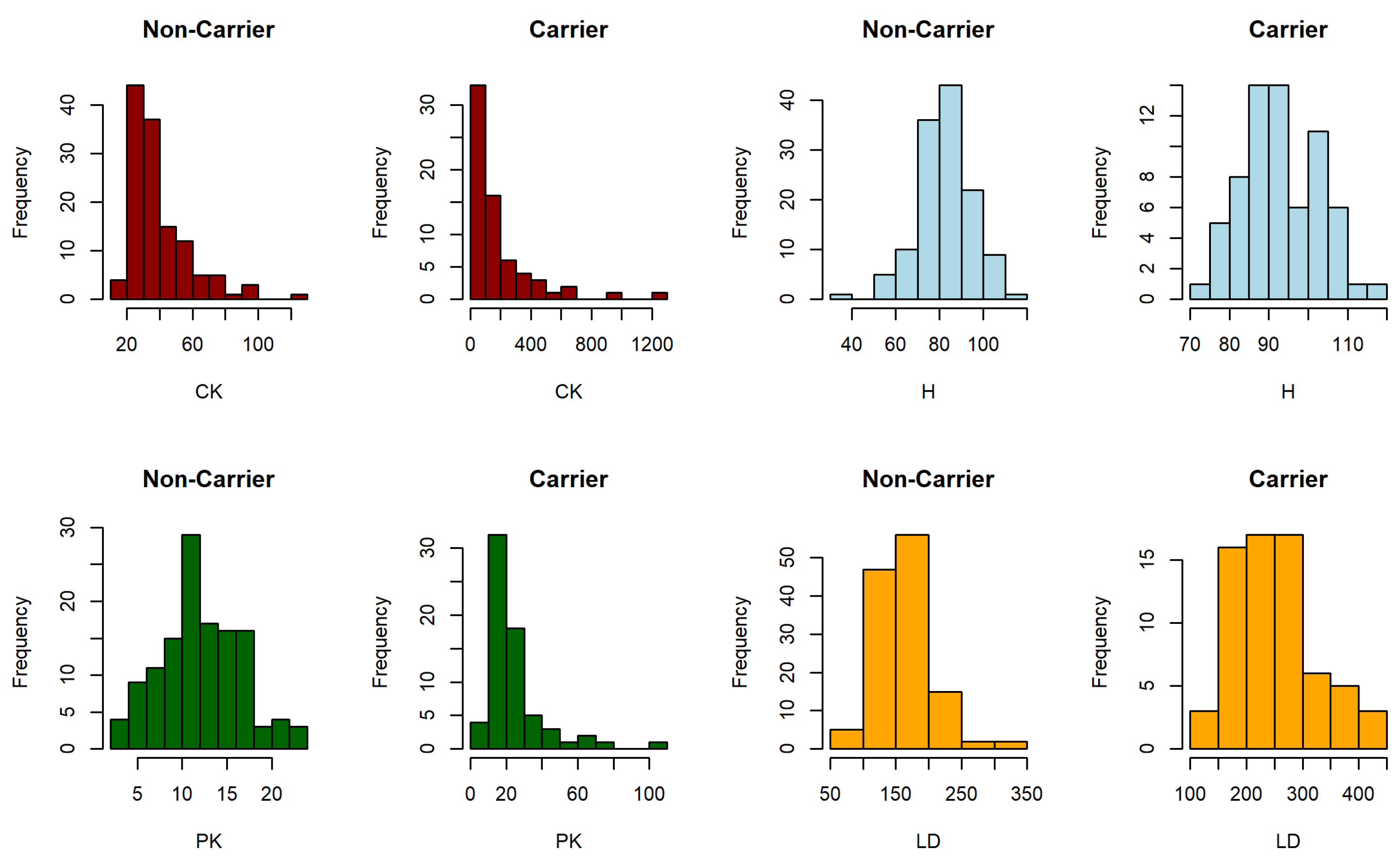
3.4.1. Duchenne Muscular Dystrophy Dataset
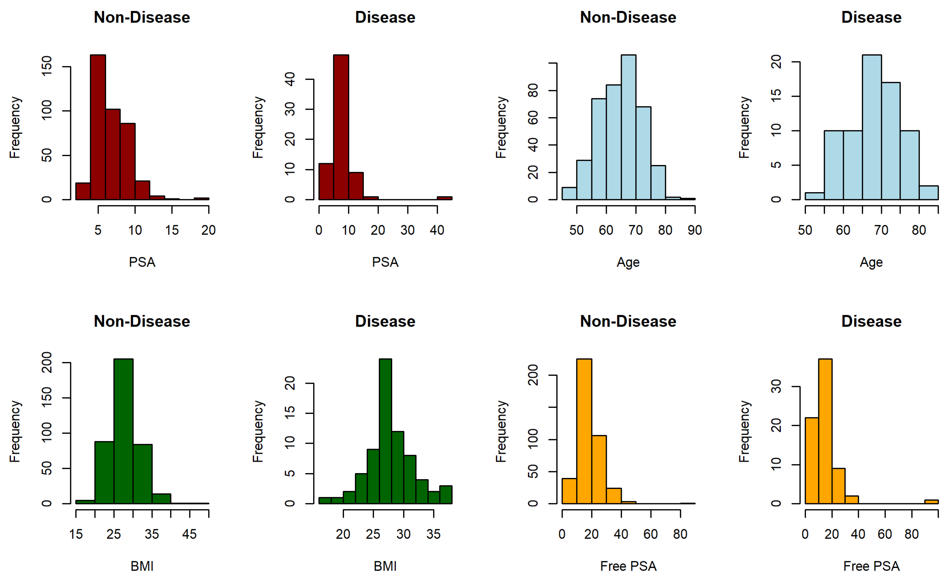
3.4.2. Prostate Cancer Dataset
4. Discussion
5. Conclusions
Author Contributions
Funding
Institutional Review Board Statement
Informed Consent Statement
Data Availability Statement
Acknowledgments
Conflicts of Interest
References
- Esteban, L.M.; Sanz, G.; Borque, A. Linear combination of biomarkers to improve diagnostic accuracy in prostate cancer. Monografías Matemáticas García de Galdeano 2013, 38, 75–84. [Google Scholar]
- Bansal, A.; Pepe, M.S. When does combining markers improve classification performance and what are implications for practice? Stat. Med. 2013, 32, 1877–1892. [Google Scholar] [CrossRef] [PubMed] [Green Version]
- Yan, L.; Tian, L.; Liu, S. Combining large number of weak biomarkers based on AUC. Stat. Med. 2015, 34, 3811–3830. [Google Scholar] [CrossRef] [Green Version]
- Lyu, T.; Ying, Z.; Zhang, H. A new semiparametric transformation approach to disease diagnosis with multiple biomarkers. Stat. Med. 2019, 38, 1386–1398. [Google Scholar] [CrossRef]
- Amini, M.; Kazemnejad, A.; Zayeri, F.; Amirian, A.; Kariman, N. Application of adjusted-receiver operating characteristic curve analysis in combination of biomarkers for early detection of gestational diabetes mellitus. Koomesh 2019, 21, 751–758. [Google Scholar]
- Ma, H.; Yang, J.; Xu, S.; Liu, C.; Zhang, Q. Combination of multiple functional markers to improve diagnostic accuracy. J. Appl. Stat. 2022, 49, 44–63. [Google Scholar] [CrossRef]
- Yu, S. A Covariate-Adjusted Classification Model for Multiple Biomarkers in Disease Screening and Diagnosis. Ph.D. Thesis, Kansas State University, Manhattan, AR, USA, 2019. [Google Scholar]
- Ahmadian, R.; Ercan, I.; Sigirli, D.; Yildiz, A. Combining binary and continuous biomarkers by maximizing the area under the receiver operating characteristic curve. Commun. Stat. Simul. Comput. 2020, 1–14. [Google Scholar] [CrossRef]
- Hu, X.; Li, C.; Chen, J.; Qin, G. Confidence intervals for the Youden index and its optimal cut-off point in the presence of covariates. J. Biopharm. Stat. 2021, 31, 251–272. [Google Scholar] [CrossRef]
- Kang, L.; Xiong, C.; Crane, P.; Tian, L. Linear combinations of biomarkers to improve diagnostic accuracy with three ordinal diagnostic categories. Stat. Med. 2013, 32, 631–643. [Google Scholar] [CrossRef] [Green Version]
- Maiti, R.; Li, J.; Das, P.; Feng, L.; Hausenloy, D.; Chakraborty, B. A distribution-free smoothed combination method of biomarkers to improve diagnostic accuracy in multi-category classification. arXiv 2019, arXiv:1904.10046. [Google Scholar]
- Su, J.Q.; Liu, J.S. Linear combinations of multiple diagnostic markers. J. Am. Stat. Assoc. 1993, 88, 1350–1355. [Google Scholar] [CrossRef]
- Pepe, M.S.; Thompson, M.L. Combining diagnostic test results to increase accuracy. Biostatistics 2000, 1, 123–140. [Google Scholar] [CrossRef] [PubMed]
- Hanley, J.A.; McNeil, B.J. The meaning and use of the area under a receiver operating characteristic (ROC) curve. Radiology 1982, 143, 29–36. [Google Scholar] [CrossRef] [PubMed] [Green Version]
- Liu, C.; Liu, A.; Halabi, S. A min–max combination of biomarkers to improve diagnostic accuracy. Stat. Med. 2011, 30, 2005–2014. [Google Scholar] [CrossRef] [PubMed] [Green Version]
- Pepe, M.S.; Cai, T.; Longton, G. Combining predictors for classification using the area under the receiver operating characteristic curve. Biometrics 2006, 62, 221–229. [Google Scholar] [CrossRef]
- Esteban, L.M.; Sanz, G.; Borque, A. A step-by-step algorithm for combining diagnostic tests. J. Appl. Stat. 2011, 38, 899–911. [Google Scholar] [CrossRef]
- Kang, L.; Liu, A.; Tian, L. Linear combination methods to improve diagnostic/prognostic accuracy on future observations. Stat. Methods Med. Res. 2016, 25, 1359–1380. [Google Scholar] [CrossRef] [Green Version]
- Liu, A.; Schisterman, E.F.; Zhu, Y. On linear combinations of biomarkers to improve diagnostic accuracy. Stat. Med. 2005, 24, 37–47. [Google Scholar] [CrossRef]
- Yin, J.; Tian, L. Joint inference about sensitivity and specificity at the optimal cut-off point associated with Youden index. Comput. Stat. Data Anal. 2014, 77, 1–13. [Google Scholar] [CrossRef]
- Yu, W.; Park, T. Two simple algorithms on linear combination of multiple biomarkers to maximize partial area under the ROC curve. Comput. Stat. Data Anal. 2015, 88, 15–27. [Google Scholar] [CrossRef]
- Yan, Q.; Bantis, L.E.; Stanford, J.L.; Feng, Z. Combining multiple biomarkers linearly to maximize the partial area under the ROC curve. Stat. Med. 2018, 37, 627–642. [Google Scholar] [CrossRef] [PubMed]
- Ma, H.; Halabi, S.; Liu, A. On the use of min-max combination of biomarkers to maximize the partial area under the ROC curve. J. Probab. Stat. 2019, 2019, 8953530. [Google Scholar] [CrossRef] [PubMed] [Green Version]
- Perkins, N.J.; Schisterman, E.F. The inconsistency of “optimal” cutpoints obtained using two criteria based on the receiver operating characteristic curve. Am. J. Epidemiol. 2006, 163, 670–675. [Google Scholar] [CrossRef] [PubMed] [Green Version]
- Youden, W.J. Index for rating diagnostic tests. Cancer J. 1950, 3, 32–35. [Google Scholar] [CrossRef]
- Martínez-Camblor, P.; Pardo-Fernández, J.C. The Youden Index in the Generalized Receiver Operating Characteristic Curve Context. Int. J. Biostat. 2019, 15, 20180060. [Google Scholar] [CrossRef]
- Yin, J.; Tian, L. Optimal linear combinations of multiple diagnostic biomarkers based on Youden index. Stat. Med. 2014, 33, 1426–1440. [Google Scholar] [CrossRef]
- Yin, J.; Tian, L. Joint confidence region estimation for area under ROC curve and Youden index. Stat. Med. 2014, 33, 985–1000. [Google Scholar] [CrossRef]
- R Core Team. R: A Language and Environment for Statistical Computing; R Foundation for Statistical Computing: Vienna, Austria, 2020; Available online: http://www.r-project.org/index.html (accessed on 19 February 2022).
- SLModels: Stepwise Linear Models for Binary Classification Problems under Youden Index Optimisation. R Package Version 0.1.2. Available online: https://cran.r-project.org/web/packages/SLModels/index.html (accessed on 19 February 2022).
- Walker, S.H.; Duncan, D.B. Estimation of the probability of an event as a function of several independent variables. Biometrika 1967, 54, 167–179. [Google Scholar] [CrossRef]
- Schisterman, E.F.; Perkins, N. Confidence intervals for the Youden index and corresponding optimal cut-point. Commun. Stat. Simul. Comput. 2007, 36, 549–563. [Google Scholar] [CrossRef]
- Faraggi, D.; Reiser, B. Estimation of the area under the ROC curve. Stat. Med. 2002, 21, 3093–3106. [Google Scholar] [CrossRef]
- Rosenblatt, M. Remarks on some nonparametric estimates of a density function. Ann. Math. Stat. 1956, 27, 832–837. [Google Scholar] [CrossRef]
- Parzen, E. On estimation of a probability density function and mode. Ann. Math. Stat. 1962, 33, 1065–1076. [Google Scholar] [CrossRef]
- Fluss, R.; Faraggi, D.; Reiser, B. Estimation of the Youden Index and its associated cutoff point. Biom. J. J. Math. Biol. 2005, 47, 458–472. [Google Scholar] [CrossRef] [PubMed] [Green Version]
- Silverman, B.W. Density Estimation for Statistics and Data Analysis; Routledge: London, UK, 2018. [Google Scholar]
- Percy, M.E.; Andrews, D.F.; Thompson, M.W. Duchenne muscular dystrophy carrier detection using logistic discrimination: Serum creatine kinase, hemopexin, pyruvate kinase, and lactate dehydrogenase in combination. Am. J. Med. Genet. A 1982, 13, 27–38. [Google Scholar] [CrossRef] [PubMed]
- Sung, H.; Ferlay, J.; Siegel, R.L.; Laversanne, M.; Soerjomataram, I.; Jemal, A.; Bray, F. Global cancer statistics 2020: GLOBOCAN estimates of incidence and mortality worldwide for 36 cancers in 185 countries. CA Cancer J. Clin. 2021, 71, 209–249. [Google Scholar] [CrossRef]
- Rubio-Briones, J.; Borque-Fernando, A.; Esteban, L.M.; Mascarós, J.M.; Ramírez-Backhaus, M.; Casanova, J.; Collado, A.; Mir, C.; Gómez-Ferrer, A.; Wong, A.; et al. Validation of a 2-gene mRNA urine test for the detection of >=GG2 prostate cancer in an opportunistic screening population. Prostate 2020, 80, 500–507. [Google Scholar] [CrossRef]
- Morote, J.; Schwartzman, I.; Borque, A.; Esteban, L.M.; Celma, A.; Roche, S.; de Torres, I.M.; Mast, R.; Semidey, M.E.; Regis, L.; et al. Prediction of clinically significant prostate cancer after negative prostate biopsy: The current value of microscopic findings. In Urologic Oncology: Seminars and Original Investigations; Elsevier: Amsterdam, The Netherlands, 2020. [Google Scholar]
- Pinsky, P.F.; Zhu, C.S. Building Multi-Marker Algorithms for Disease Prediction—The Role of Correlations among Markers. Biomark. Insights 2011, 6, 83–93. [Google Scholar] [CrossRef]
- Rota, M.; Antolini, L. Finding the optimal cut-point for Gaussian and Gamma distributed biomarkers. Comput. Stat. Data Anal. 2014, 69, 1–14. [Google Scholar] [CrossRef]
- Bellman, R.E. Dynamic Programming; Princeton University Press: Princeton, NJ, USA, 1957. [Google Scholar]
- Aznar-Gimeno, R.; Esteban, L.M.; Sanz, G.; del-Hoyo-Alonso, R.; Savirón-Cornudella, R.; Antolini, L. Incorporating a New Summary Statistic into the Min–Max Approach: A Min–Max–Median, Min–Max–IQR Combination of Biomarkers for Maximising the Youden Index. Mathematics 2021, 9, 2497. [Google Scholar] [CrossRef]
| Size () | Independence () | |||||
|---|---|---|---|---|---|---|
| SLM | SWD | MM | LR | MVN | KS | |
| (50, 50) | 0.4270 (0.0951) | 0.4206 (0.1134) | 0.3696 (0.1037) | 0.4530 (0.0919) | 0.4520 (0.0934) | 0.4434 (0.0911) |
| (500, 500) | 0.4823 (0.0304) | 0.4804 (0.0291) | 0.4103 (0.0308) | 0.4882 (0.0282) | 0.4895 (0.0297) | 0.4863 (0.0301) |
| (50, 50) | 0.6610 (0.0842) | 0.6610 (0.0880) | 0.6024 (0.0908) | 0.6990 (0.0779) | 0.6994 (0.0787) | 0.6902 (0.0773) |
| (500, 500) | 0.7163 (0.0224) | 0.7159 (0.0228) | 0.6418 (0.0253) | 0.7238 (0.0205) | 0.7249 (0.0200) | 0.7223 (0.0207) |
| Low correlation (··J) | ||||||
| SLM | SWD | MM | LR | MVN | KS | |
| (50, 50) | 0.3430 (0.0969) | 0.3376 (0.1041) | 0.2642 (0.1211) | 0.3686 (0.0949) | 0.3736 (0.0924) | 0.3586 (0.1012) |
| (500, 500) | 0.4074 (0.0285) | 0.4056 (0.0303) | 0.3189 (0.0322) | 0.4149 (0.0309) | 0.4155 (0.0314) | 0.4131 (0.0292) |
| (50, 50) | 0.5576 (0.0939) | 0.5510 (0.1024) | 0.5056 (0.0979) | 0.5790 (0.0921) | 0.5790 (0.0853) | 0.5740 (0.0955) |
| (500, 500) | 0.6084 (0.0294) | 0.6079 (0.0284) | 0.5213 (0.0289) | 0.6183 (0.0286) | 0.6181 (0.0284) | 0.6161 (0.0289) |
| Medium correlation (··J) | ||||||
| SLM | SWD | MM | LR | MVN | KS | |
| (50, 50) | 0.3618 (0.0984) | 0.3442 (0.1009) | 0.2474 (0.1072) | 0.3750 (0.0854) | 0.3678 (0.0839) | 0.3640 (0.0880) |
| (500, 500) | 0.4088 (0.0351) | 0.4039 (0.0327) | 0.2924 (0.0323) | 0.4178 (0.0334) | 0.4189 (0.0340) | 0.4154 (0.0336) |
| (50, 50) | 0.5490 (0.0921) | 0.5340 (0.1002) | 0.4584 (0.0994) | 0.5660 (0.0830) | 0.5684 (0.0864) | 0.5584 (0.0876) |
| (500, 500) | 0.5936 (0.0303) | 0.5914 (0.0303) | 0.4840 (0.0293) | 0.6063 (0.0319) | 0.6059 (0.0301) | 0.6034 (0.0286) |
| High correlation (··J) | ||||||
| SLM | SWD | MM | LR | MVN | KS | |
| (50, 50) | 0.4150 (0.0946) | 0.3430 (0.1203) | 0.2522 (0.1081) | 0.4296 (0.0952) | 0.4310(0.0989) | 0.4136 (0.0962) |
| (500, 500) | 0.4588 (0.0307) | 0.4234 (0.0386) | 0.2899 (0.0317) | 0.4662 (0.0260) | 0.4666 (0.0258) | 0.4632 (0.0280) |
| (50, 50) | 0.5892 (0.09036) | 0.5364 (0.1098) | 0.4542 (0.0957) | 0.6218 (0.0839) | 0.6196 (0.0851) | 0.6134 (0.0892) |
| (500, 500) | 0.6285 (0.0234) | 0.6171 (0.0307) | 0.4823 (0.0315) | 0.6456 (0.0220) | 0.6461 (0.0213) | 0.6460 (0.0227) |
| Size () | Different Correlation (····J) | |||||
|---|---|---|---|---|---|---|
| SLM | SWD | MM | LR | MVN | KS | |
| (50, 50) | 0.3528 (0.1106) | 0.3532 (0.1072) | 0.3236 (0.1012) | 0.3878 (0.1079) | 0.3814 (0.1061) | 0.3832 (0.1127) |
| (500, 500) | 0.4162 (0.0278) | 0.4128 (0.0318) | 0.3534 (0.0329) | 0.4224 (0.0282) | 0.4233 (0.0295) | 0.4120 (0.0281) |
| (50, 50) | 0.5500 (0.1030) | 0.5218 (0.1041) | 0.4328 (0.0880) | 0.5792 (0.1014) | 0.5730 (0.1012) | 0.5700 (0.1025) |
| (500, 500) | 0.5974 (0.0295) | 0.5966 (0.0299) | 0.4757 (0.0320) | 0.6062 (0.0276) | 0.6053 (0.0275) | 0.6038 (0.0271) |
| Size () | Negative Correlation (−0.1) | |||||
|---|---|---|---|---|---|---|
| SLM | SWD | MM | LR | MVN | KS | |
| (50, 50) | 0.4822 (0.0990) | 0.4670 (0.1028) | 0.4316 (0.0939) | 0.5168 (0.0944) | 0.5160 (0.0920) | 0.5010 (0.0920) |
| (500, 500) | 0.5457 (0.0263) | 0.5452 (0.0268) | 0.4631 (0.0296) | 0.5545 (0.0255) | 0.5558 (0.0264) | 0.5504 (0.0275) |
| (50, 50) | 0.7444 (0.0800) | 0.7388 (0.0725) | 0.6788 (0.0874) | 0.7694 (0.0671) | 0.7730 (0.0653) | 0.7702 (0.0611) |
| (500, 500) | 0.7960 (0.0209) | 0.7953 (0.0213) | 0.7085 (0.0265) | 0.8015 (0.0204) | 0.8015 (0.0216) | 0.7990 (0.0194) |
| Negative correlation (−0.3) | ||||||
| SLM | SWD | MM | LR | MVN | KS | |
| (50, 50) | 0.8696 (0.0790) | 0.8046 (0.1118) | 0.6602 (0.0787) | 0.9210 (0.0426) | 0.9284 (0.0374) | 0.9198 (0.0444) |
| (500,500) | 0.9192 (0.0242) | 0.9107 (0.0278) | 0.6930 (0.0239) | 0.9424 (0.0110) | 0.9423 (0.0117) | 0.9417 (0.0114) |
| (50, 50) | 0.9382 (0.0600) | 0.9462 (0.0485) | 0.8754 (0.0545) | 0.9544 (0.0410) | 0.9734 (0.0338) | 0.9646 (0.0443) |
| (500,500) | 0.9950 (0.0043) | 0.9943 (0.0047) | 0.9001 (0.0153) | 0.9948 (0.0049) | 0.9975 (0.0030) | 0.9958 (0.0047) |
| Size () | Same Means () | |||||
|---|---|---|---|---|---|---|
| SLM | SWD | MM | LR | MVN | KS | |
| Same Correlation. Low Correlation (··J) | ||||||
| (50, 50) | 0.4626 (0.1062) | 0.4376 (0.1081) | 0.4794 (0.0954) | 0.4878 (0.0900) | 0.4882 (0.0944) | 0.4852 (0.0951) |
| (500, 500) | 0.5129 (0.0305) | 0.5174 (0.0318) | 0.5073 (0.0278) | 0.5254 (0.0285) | 0.5254 (0.0284) | 0.5219 (0.0283) |
| Different Correlation (····J) | ||||||
| (50, 50) | 0.4030 (0.1110) | 0.4102 (0.1057) | 0.5220 (0.0966) | 0.4340 (0.1029) | 0.4402 (0.1027) | 0.4312 (0.1018) |
| (500, 500) | 0.4726 (0.0281) | 0.4697 (0.0280) | 0.5609 (0.0285) | 0.4783 (0.0259) | 0.4793 (0.0260) | 0.4753 (0.0256) |
| Size () | Different Marginal Distributions | |||||
|---|---|---|---|---|---|---|
| SLM | SWD | MM | LR | MVN | KS | |
| (50, 50) | 0.4732 (0.0860) | 0.4684 (0.0891) | 0.2374 (0.1158) | 0.3656 (0.1243) | 0.3316 (0.1534) | 0.3146 (0.2140) |
| (500, 500) | 0.5095 (0.0277) | 0.5018 (0.0297) | 0.3180 (0.0442) | 0.4137 (0.0459) | 0.4285 (0.0671) | 0.4787 (0.1191) |
| (50, 50) | 0.7058 (0.0848) | 0.6794 (0.0877) | 0.3716 (0.1194) | 0.6572 (0.1080) | 0.6368 (0.1079) | 0.6716 (0.1207) |
| (500, 500) | 0.7568 (0.0231) | 0.7351 (0.0229) | 0.4350 (0.04530) | 0.7065 (0.0363) | 0.6807 (0.0360) | 0.7469 (0.0304) |
| Size () | Log-Normal Distributions | |||||
|---|---|---|---|---|---|---|
| SLM | SWD | MM | LR | MVN | KS | |
| Different means: . Independence () | ||||||
| (50, 50) | 0.4022 (0.1019) | 0.4078 (0.1041) | 0.3658 (0.1060) | 0.4112 (0.0936) | 0.4034 (0.0903) | 0.3914 (0.1142) |
| (500, 500) | 0.4504 (0.0296) | 0.4506 (0.0315) | 0.4096 (0.0324) | 0.4562 (0.0300) | 0.4541 (0.0321) | 0.4507 (0.0534) |
| Different means: . Medium correlation (··J) | ||||||
| (50, 50) | 0.3460 (0.0103) | 0.3454 (0.1056) | 0.2574 (0.1024017) | 0.3482 (0.1065) | 0.3370 (0.1100) | 0.3374 (0.1133) |
| (500, 500) | 0.3990 (0.0345) | 0.3954 (0.0358) | 0.2924 (0.0336) | 0.3990 (0.0372) | 0.3960 (0.0367) | 0.4014 (0.0348) |
| Same means: . Medium correlation (··J) | ||||||
| (50, 50) | 0.3890 (0.1035) | 0.3756 (0.1029) | 0.4170 (0.1046) | 0.4102 (0.0969) | 0.3796 (0.1187) | 0.3584 (0.1133) |
| (500, 500) | 0.4465 (0.0306) | 0.4515 (0.0315) | 0.4548 (0.0282) | 0.4570 (0.0309) | 0.4514 (0.0317) | 0.4545 (0.0317) |
| Computational Times (min) | ||||||
|---|---|---|---|---|---|---|
| SLM | SWD | MM | LR | MVN | KS | |
| 17.1157 | 0.096 | 0.014 | 0.00003 | 0.00004 | 0.0003 | |
| 0.5939 | 0.096 | 0.033 | 0.00004 | 0.00004 | 0.0007 | |
| Non-Carrier | Carrier | |||||
|---|---|---|---|---|---|---|
| Youden | Threshold | Mean | SD | Mean | SD | |
| CK | 0.6124 | 57 | 36.6102 | 18.6006 | 185.791 | 226.9330 |
| H | 0.4172 | 87.5 | 82.3072 | 12.2403 | 92.9303 | 9.8576 |
| PK | 0.5079 | 16.7 | 12.1447 | 4.3935 | 23.9310 | 17.2122 |
| LD | 0.5776 | 188 | 164.5748 | 41.3686 | 250.9403 | 72.4368 |
| Correlations | ||||||
| Non-Carrier | ||||||
| −0.3340 | 0.1029 | 0.1987 | 0.0812 | 0.1824 | 0.2188 | |
| Carrier | ||||||
| −0.1364 | 0.6953 | 0.4851 | −0.118 | −0.1048 | 0.4813 | |
| Non-Cancer | Cancer | |||||
|---|---|---|---|---|---|---|
| Youden | Threshold | Mean | SD | Mean | SD | |
| PSA | 0.1571 | 9.45 | 6.7875 | 2.3160 | 7.9887 | 5.2761 |
| Age | 0.2202 | 68 | 65.0804 | 7.2840 | 68.8732 | 6.6846 |
| BMI | 0.0953 | 25.83 | 27.8590 | 3.8243 | 27.7559 | 3.8756 |
| Free PSA | 0.4007 | 13.95 | 18.3629 | 7.5917 | 14.7190 | 11.4067 |
| Correlations | ||||||
| Non-Cancer | ||||||
| 0.0901 | −0.1179 | −0.1127 | 0.0536 | 0.0894 | 0.0694 | |
| Cancer | ||||||
| −0.1985 | 0.0896 | −0.0756 | 0.0758 | 0.2478 | −0.0767 | |
| Optimal Linear Combination | Youden | Sensitivity | Specificity | |
|---|---|---|---|---|
| SLM | 0.8255 | 0.8806 | 0.9449 | |
| SWD | 0.8184 | 0.8657 | 0.9528 | |
| MM | 0.7335 | 0.8358 | 0.8976 | |
| LR | 0.8106 | 0.8657 | 0.9449 | |
| MVN | 0.7878 | 0.8507 | 0.9370 | |
| KS | 0.8035 | 0.8507 | 0.9528 |
| Optimal Linear Combination | Youden | Sensitivity | Specificity | |
|---|---|---|---|---|
| SLM | 0.4857 | 0.7746 | 0.7111 | |
| SWD | 0.4319 | 0.7887 | 0.6432 | |
| MM | 0.2986 | 0.5775 | 0.7211 | |
| LR | 0.4284 | 0.7324 | 0.6960 | |
| MVN | 0.3660 | 0.6901 | 0.6759 | |
| KS | 0.4681 | 0.7746 | 0.6935 |
| 10-Fold Cross Validation. DMD Dataset. | |||
|---|---|---|---|
| Youden | Sensitivity | Specificity | |
| SLM | 0.7611 | 0.8576 | 0.9135 |
| SWD | 0.7301 | 0.8167 | 0.9135 |
| MM | 0.6215 | 0.7786 | 0.8429 |
| LR | 0.7861 | 0.8476 | 0.9345 |
| MVN | 0.7391 | 0.8167 | 0.9224 |
| KS | 0.7635 | 0.8333 | 0.9301 |
| 10-Fold Cross Validation. Prostate Dataset. | |||
|---|---|---|---|
| Youden | Sensitivity | Specificity | |
| SLM | 0.3844 | 0.6786 | 0.7058 |
| SWD | 0.3628 | 0.6946 | 0.6681 |
| MM | 0.2247 | 0.4661 | 0.7586 |
| LR | 0.3327 | 0.6768 | 0.6559 |
| MVN | 0.2785 | 0.6625 | 0.6160 |
| KS | 0.3820 | 0.6911 | 0.6910 |
Publisher’s Note: MDPI stays neutral with regard to jurisdictional claims in published maps and institutional affiliations. |
© 2022 by the authors. Licensee MDPI, Basel, Switzerland. This article is an open access article distributed under the terms and conditions of the Creative Commons Attribution (CC BY) license (https://creativecommons.org/licenses/by/4.0/).
Share and Cite
Aznar-Gimeno, R.; Esteban, L.M.; del-Hoyo-Alonso, R.; Borque-Fernando, Á.; Sanz, G. A Stepwise Algorithm for Linearly Combining Biomarkers under Youden Index Maximization. Mathematics 2022, 10, 1221. https://doi.org/10.3390/math10081221
Aznar-Gimeno R, Esteban LM, del-Hoyo-Alonso R, Borque-Fernando Á, Sanz G. A Stepwise Algorithm for Linearly Combining Biomarkers under Youden Index Maximization. Mathematics. 2022; 10(8):1221. https://doi.org/10.3390/math10081221
Chicago/Turabian StyleAznar-Gimeno, Rocío, Luis M. Esteban, Rafael del-Hoyo-Alonso, Ángel Borque-Fernando, and Gerardo Sanz. 2022. "A Stepwise Algorithm for Linearly Combining Biomarkers under Youden Index Maximization" Mathematics 10, no. 8: 1221. https://doi.org/10.3390/math10081221
APA StyleAznar-Gimeno, R., Esteban, L. M., del-Hoyo-Alonso, R., Borque-Fernando, Á., & Sanz, G. (2022). A Stepwise Algorithm for Linearly Combining Biomarkers under Youden Index Maximization. Mathematics, 10(8), 1221. https://doi.org/10.3390/math10081221