Article

Effects of the Wiener Process on the Solutions of the Stochastic Fractional Zakharov System

by
Farah M. Al-Askar
1,
Wael W. Mohammed
2,3,*,
Mohammad Alshammari
2 and
M. El-Morshedy
4,5
1
Department of Mathematical Science, Collage of Science, Princess Nourah Bint, Abdulrahman University, P.O. Box 84428, Riyadh 11671, Saudi Arabia
2
Department of Mathematics, Faculty of Science, University of Ha’il, Ha’il 2440, Saudi Arabia
3
Department of Mathematics, Faculty of Science, Mansoura University, Mansoura 35516, Egypt
4
Department of Mathematics, College of Science and Humanities in Al-Kharj, Prince Sattam Bin Abdulaziz University, Al-Kharj 11942, Saudi Arabia
5
Department of Statistics and Computer Science, Faculty of Science, Mansoura University, Mansoura 35516, Egypt
*
Author to whom correspondence should be addressed.
Mathematics 2022, 10(7), 1194; https://doi.org/10.3390/math10071194
Submission received: 16 March 2022 / Revised: 1 April 2022 / Accepted: 2 April 2022 / Published: 6 April 2022
(This article belongs to the Special Issue Applications of Partial Differential Equations)

Abstract

:
We consider in this article the stochastic fractional Zakharov system derived by the multiplicative Wiener process in the Stratonovich sense. We utilize two distinct methods, the Riccati–Bernoulli sub-ODE method and Jacobi elliptic function method, to obtain new rational, trigonometric, hyperbolic, and elliptic stochastic solutions. The acquired solutions are helpful in explaining certain fascinating physical phenomena due to the importance of the Zakharov system in the theory of turbulence for plasma waves. In order to show the influence of the multiplicative Wiener process on the exact solutions of the Zakharov system, we employ the MATLAB tools to plot our figures to introduce a number of 2D and 3D graphs. We establish that the multiplicative Wiener process stabilizes the solutions of the Zakharov system around zero.

1. Introduction

In 1972, Zakharov [1] developed the Zakharov system. It is a group of coupled nonlinear wave equations that explains the interaction of high-frequency Langmuir (dispersive) and low-frequency ion-acoustic (roughly nondispersive) waves. In one dimension, the Zakharov system can be authored as
v t t v x x + ( u 2 ) x x = 0 , i u t + u x x + 2 u v = 0 ,
where v : Ω × R + R denotes the plasma density as determined by its equilibrium value, and u : Ω × R + C denotes the high-frequency electric field’s envelope. The Zakharov system is similar to nonlinear Schrödinger equations and significant in plasma turbulence theory. As a result, the Zakharov system has piqued the interest of many physicists and mathematicians, and has been extensively studied both theoretically and numerically [2,3,4,5,6]. To solve system problems (1), researchers have used a variety of methods. For example, Song et al. [7] introduced unbounded wave solutions, kink wave solutions, and periodic wave solutions by utilizing bifurcation theory method. Wang and Li [8] used the extended F-expansion method to obtain periodic wave solutions. Javidi et al. [9] applied the variational iteration technique to obtain solitary wave solutions. Taghizadeh et al. [10] obtained some exact solutions using infinite series method. Hong et al. [11] obtained a few new doubly periodic solutions utilizing the Jacobian elliptic function expansion method.
In recent years, the fractional derivatives are utilized to describe numerous physical phenomena in engineering applications, signal processing, electromagnetic theory, finance, physics, mathematical biology, and various scientific studies, see for instance [12,13,14,15,16,17]. For instance, the fractional derivative is utilized in control theory, controller tuning, optics, seismic wave analysis, dynamical system, signal processing, and viscoelasticity.
On the other hand, the benefits of taking random effects into consideration in predicting, simulating, analyzing and modeling complex phenomena has been extensively distinguished in biology, engineering, physics, geophysical, chemistry, climate dynamics, and other fields [18,19,20,21]. Stochastic partial differential equations (SPDEs) are suitable mathematical equations for complicated systems subject to noise or random influences. Normally, random influences can be thought of as a simple estimate of turbulence in fluids. Therefore, we have to generalize the Zakharov system by taking into account more elements due to some important effects such as ion nonlinearities and transit-time damping.
To achieve a higher level of qualitative agreement, we consider here the following stochastic fractional-space Zakharov system (SFSZS) with multiplicative noise in the Stratonovich sense:
i u t + T x x α u + 2 u v + i σ u W t = 0 ,
v t t T x x α v + T x x α ( u 2 ) = 0 ,
where T α is the conformable fractional derivative (CFD) [22], W ( t ) is standard Wiener process (SWP).
In [23,24], the stochastic dissipative Zakharov system are obtained by utilizing the global-random attractors provided with normal topology, while in [25], the uniqueness and existence of solutions of the Zakharov system with stochastic term are obtained by applying the method of Galerkin approximation.
The novelty of this paper is to construct the exact fractional stochastic solutions of the SFSZS (2)–(3). This study is the first one to obtain the exact solutions of the SFSZS (2)–(3). We use two distinct methods including the Jacobi elliptic function and the Riccati–Bernoulli sub-ODE to achieve a wide range of solutions, including hyperbolic, trigonometric, rational, and elliptic functions. Besides that, we employ Matlab tools to plot 3D and 2D graphs for some of the analytical solutions developed in this study to check the effect of the Wiener process on the solutions of SFSZS (2)–(3).
The following is how the paper is arranged. In Section 2, we define the CFD and Wiener process and we state some features about them. To obtain the wave equation of SFSZS (2)–(3), we use a suitable wave transformation in Section 3. In Section 4, we apply two different methods to construct the exact solutions of SFSZS (2)–(3). In Section 5, we study the effect of the SWP on the obtained solutions. Finally, we present the paper’s conclusion.

2. Preliminaries

In this section, we introduce some definitions and features for CFD, which are reported in [22] and SWP.
Definition 1.
Assume f : ( 0 , ) R ; hence, the CFD of f of order α is defined as
T x α f ( x ) = lim h 0 f ( x + h x 1 α ) f ( x ) h .
Theorem 1.
Let f , g : ( 0 , ) R be differentiable, and also α differentiable functions; then, the next rule holds:
T x α ( f g ) ( x ) = x 1 α g ( x ) f ( g ( x ) ) .
Let us state some properties of the CFD:
  • T x α [ a f ( x ) + b g ( x ) ] = a T x α f ( x ) + b T x α g ( x ) , a , b R ,
  • T x α [ C ] = 0 , C is a constant,
  • T x α [ x ] = x α , R ,
  • T x α g ( x ) = x 1 α d g d x ,
In the next definition, we define standard Wiener process W ( t ) :
Definition 2.
stochastic process { W ( t ) } t 0 is called a Wiener process if it satisfies
1. 
W ( 0 ) = 0 ,
2. 
W ( t ) , t 0 is continuous function of t,
3. 
For t 1 < t 2 , W ( t 1 ) W ( t 2 ) is independent,
4. 
W ( t 2 ) W ( t 1 ) has a Gaussian distribution with mean 0 and variance t 2 t 1 .
We know the stochastic integral 0 t Θ d W may be interpreted in a variety of ways [26]. The Stratonovich and Itô interpretations of a stochastic integral are widely used. The stochastic integral is Itô (denoted by 0 t Θ d W ) when it is evaluated at the left-end, while a Stratonovich stochastic integral (denoted by 0 t Θ d W ) is one that is calculated at the midpoint. The next is the relationship between the Stratonovich and Itô integral:
0 t Θ ( τ , Z τ ) d W ( τ ) = 0 t Θ ( τ , Z τ ) d W ( τ ) 1 2 0 t Θ ( τ , Z τ ) Θ ( τ , Z τ ) z d τ ,
where Θ is supposed to be sufficiently regular and { Z t , t 0 } is a stochastic process.

3. Wave Equation for SFSZS

To acquire the wave equation for the SFSZS (2)–(3), the next wave transformation is applied:
u ( x , t ) = φ ( μ ) e ( i θ σ W ( t ) σ 2 t ) , μ = k ( 1 α x α λ t ) and θ = λ 2 α x α + ρ t ,
where φ is a deterministic function and k , λ , ρ are nonzero constants. Plugging Equation (5) into Equation (2) and using
d u d t = ( λ k φ + i ρ φ σ φ W t 1 2 σ 2 φ ) e ( i θ σ W ( t ) σ 2 t ) , = ( λ k φ + i ρ φ σ φ W t ) e ( i θ σ W ( t ) σ 2 t ) , T x x α = ( k 2 φ + i λ k φ 1 4 λ 2 φ ) e ( i θ σ W ( t ) σ 2 t ) ,
where we used (4). We obtain, for the real part,
k 2 φ ( 1 4 λ 2 + ρ ) φ + 2 φ v = 0 .
Now, we suppose
v ( x , t ) = ψ ( μ ) ,
where ψ is real deterministic function, to obtain
v t = λ k ψ , v t t = λ 2 k 2 ψ , T x x α v = k 2 ψ .
Substituting Equation (8) into Equation (3), we attain
( λ 2 1 ) ψ + ( φ 2 ) e ( 2 σ W ( t ) 2 σ 2 t ) = 0 .
Taking expectation E ( · ) on both sides, we have
( λ 2 1 ) ψ + ( φ 2 ) e 2 σ 2 t E ( e 2 σ W ( t ) ) = 0 .
Since W ( t ) is standard Gaussian process; hence, E ( e W ( t ) ) = e 2 2 t for any real constant . Now, Equation (10) has the form
( λ 2 1 ) ψ + ( φ 2 ) = 0 ,
Integrating Equation (11) twice and putting the constants of integration equal zero yields
( λ 2 1 ) ψ + φ 2 = 0 .
Hence, Equation (12) becomes
ψ = φ 2 ( λ 2 1 ) .
Putting Equation (13) into Equation (7), we obtain the next wave equation
φ γ 1 φ 3 γ 2 φ = 0 ,
where
γ 1 = 2 k 2 ( λ 2 1 ) and γ 2 = 1 4 k 2 ( λ 2 + 4 ρ ) .

4. The Analytical Solutions of the SFSZS

To find the solutions of Equation (14), we utilize two different methods: Riccati–Bernoulli sub-ODE [27] and the Jacobi elliptic function method [28]. Therefore, we acquire the analytical solutions of the SFSZS (2)–(3).

4.1. Riccati–Bernoulli Sub-ODE Method

Assume the following Riccati–Bernoulli equation:
φ = 1 φ 2 + 2 φ + 3 ,
where 1 , 2 , 3 are undefined constants and φ = φ ( μ ) .
Differentiating Equation (16) with respect to μ , we obtain
φ = 2 1 φ φ + 2 φ ,
and using Equation (16) yields
φ = 2 1 2 φ 3 + 3 1 2 φ 2 + ( 2 1 3 + 2 2 ) φ + 2 3 .
Substituting (17) into (14), we have
( 2 1 2 γ 1 ) φ 3 + 3 1 2 φ 2 + ( 2 1 3 + 2 2 γ 2 ) φ + 2 3 = 0 .
Equating each coefficient of φ i ( i = 0 , 1 , 2 , 3 ) to zero, we achieve the next algebraic equations
2 3 = 0 ,
( 2 1 3 + 2 2 γ 2 ) = 0 ,
3 1 2 = 0 ,
2 1 2 γ 1 = 0 .
When the above equations are solved, the result is
1 = ± 1 2 γ 1 , 2 = 0 , 3 = γ 2 2 1 = ± γ 2 2 γ 1 .
There are numerous solutions to the Riccati–Bernoulli Equation (16) depending on 1 and 3 .
First case: If 3 1 = 0 , then Riccati–Bernoulli Equation (16) has the solution
φ ( μ ) = 1 1 μ + C .
Hence, the SFSZS (2)–(3) has the analytical solutions
u ( x , t ) = φ ( μ ) e ( i θ σ W ( t ) σ 2 t ) = 1 1 ( k α x α k λ t ) + C e ( i θ σ W ( t ) σ 2 t ) ,
v ( x , t ) = φ 2 ( λ 2 1 ) = 1 ( λ 2 1 ) 1 ( k α x α k λ t ) + C 2 .
Second case: If 3 1 > 0 , then the Riccati–Bernoulli equation (16) has the solution
φ ( μ ) = 3 1 tan 3 1 ( 1 μ + C ) ,
or
φ ( μ ) = 3 1 cot 3 1 ( 1 μ + C ) .
Therefore, SFSZSs (2)–(3) have the following solutions:
u ( x , t ) = e ( i θ σ W ( t ) σ 2 t ) 3 1 tan 3 1 ( 1 ( k α x α k λ t ) + C ) ,
v ( x , t ) = 3 ( λ 2 1 ) 1 tan 2 3 1 ( 1 ( k α x α k λ t ) + C ) ,
or
u ( x , t ) = e ( i θ σ W ( t ) σ 2 t ) 3 1 cot 3 1 ( 1 ( k α x α k λ t ) + C ) ,
v ( x , t ) = 3 ( λ 2 1 ) 1 cot 2 3 1 ( 1 ( k α x α k λ t ) + C ) ,
respectively.
Third case: If 3 1 < 0 and φ < 3 1 , then Riccati–Bernoulli Equation (16) has the solution
φ ( μ ) = 3 1 tanh 3 1 ( 1 μ + C ) .
Thus, the SFSZS (2)–(3) have the following analytical solutions:
u ( x , t ) = e ( i θ σ W ( t ) σ 2 t ) 3 1 tanh 3 1 ( 1 ( k α x α k λ t ) + C ) ,
v ( x , t ) = 3 ( λ 2 1 ) 1 tanh 2 3 1 ( 1 ( k α x α k λ t ) + C ) .
Fourth case: If 3 1 < 0 and φ 2 > 3 1 , then Riccati–Bernoulli Equation (16) has the solution
φ ( μ ) = 3 1 coth 3 1 ( 1 μ + C ) .
Consequently, the analytical solutions of the SFSZS (2)–(3) are
u ( x , t ) = e ( i θ σ W ( t ) σ 2 t ) 3 1 coth 3 1 ( 1 ( k α x α k λ t ) + C ) ,
v ( x , t ) = 3 ( λ 2 1 ) 1 coth 2 3 1 ( 1 ( k α x α k λ t ) + C ) ,
where 1 and 2 are defined in Equation (18).

4.2. The Jacobi Elliptic Function Method

Assuming that the solutions to Equation (14) are of the form
φ ( μ ) = a + b s n ( δ μ ) ,
where s n ( δ μ ) = s n ( δ μ , m ) , for 0 < m < 1 , is the Jacobi elliptic sine function and a , b , δ are unknown constants. Differentiate Equation (29) two times and we have
φ ( μ ) = ( m 2 + 1 ) b δ 2 s n ( δ μ ) + 2 m 2 b δ 2 s n 3 ( δ μ ) .
Substituting Equations (29) and (30) into Equation (14), we attain
( 2 m 2 b δ 2 γ 1 b 3 ) s n 3 ( δ μ ) 3 γ 1 a b 2 s n 2 ( δ μ )
[ ( m 2 + 1 ) b δ 2 + 3 γ 1 a 2 b + γ 2 b ] s n ( δ μ ) ( γ 1 a 3 + a γ 2 ) = 0 .
Setting each coefficient of [ s n ( δ μ ) ] n ( n = 0 , 1 , 2 , 3 ) equal to zero, we attain
γ 1 a 3 + a γ 2 = 0 ,
( m 2 + 1 ) b δ 2 + 3 γ 1 a 2 b + γ 2 b = 0 ,
3 γ 1 a b 2 s n 2 = 0 ,
and
2 m 2 b δ 2 γ 1 b 3 = 0 .
Solving the above equations, we have
a = 0 , b = ± 2 m 2 γ 2 ( m 2 + 1 ) γ 1 δ 2 = γ 2 ( m 2 + 1 ) .
Hence, the solution of Equation (14), by using (29), has the form
φ ( μ ) = ± 2 m 2 γ 2 ( m 2 + 1 ) γ 1 s n ( γ 2 ( m 2 + 1 ) μ ) .
Therefore, the analytical solutions of the SFSZS (2)–(3) are
u ( x , t ) = ± 2 m 2 γ 2 ( m 2 + 1 ) γ 1 s n γ 2 ( m 2 + 1 ) ( k α x α k λ t ) e ( i θ σ W ( t ) σ 2 t ) ,
v ( x , t ) = k 2 m 2 γ 2 ( m 2 + 1 ) s n 2 γ 2 ( m 2 + 1 ) ( k α x α k λ t ) ,
for γ 2 < 0 and γ 1 > 0 . When m 1 , the solutions (31)–(32) transfer into
u ( x , t ) = ± γ 2 γ 1 tanh γ 2 2 ( k α x α k λ t ) e ( i θ σ W ( t ) σ 2 t ) ,
v ( x , t ) = k 2 γ 2 2 tanh 2 γ 2 2 ( k α x α k λ t ) .
Analogously, we can replace s n in (29) by c n and d n in order to obtain the solutions of Equation (14), respectively, as follows:
φ ( μ ) = ± 2 m 2 γ 2 ( 2 m 2 1 ) γ 1 c n ( γ 2 ( 2 m 2 1 ) μ ) ,
and
φ ( μ ) = ± 2 m 2 γ 2 ( 2 m 2 ) γ 1 d n ( γ 2 ( 2 m 2 ) μ ) .
Consequently, the solutions of the SFSZS (2)–(3) have the following forms:
u ( x , t ) = ± 2 m 2 γ 2 ( 2 m 2 1 ) γ 1 c n γ 2 ( 2 m 2 1 ) ( k α x α k λ t ) e ( i θ σ W ( t ) σ 2 t ) ,
v ( x , t ) = k 2 m 2 γ 2 ( 2 m 2 1 ) c n 2 γ 2 ( 2 m 2 1 ) ( k α x α k λ t ) ,
for γ 2 ( 2 m 2 1 ) < 0 , γ 1 > 0 , and
u ( x , t ) = ± 2 m 2 γ 2 ( 2 m 2 1 ) γ 1 d n γ 2 ( 2 m 2 1 ) ( k α x α k λ t ) e ( i θ σ W ( t ) σ 2 t ) ,
v ( x , t ) = k 2 m 2 γ 2 ( 2 m 2 ) d n 2 γ 2 ( 2 m 2 ) ( k α x α k λ t ) ,
for γ 2 < 0 , γ 1 > 0 , respectively. When m 1 , the solutions (35)–(36) and (37)–(38) transfer into
u ( x , t ) = ± 2 γ 2 γ 1 sec h γ 2 ( k α x α k λ t ) e ( i θ σ W ( t ) σ 2 t ) ,
v ( x , t ) = k 2 m 2 γ 2 sec h 2 γ 2 ( k α x α k λ t ) ,
for γ 2 < 0 , γ 1 > 0 .

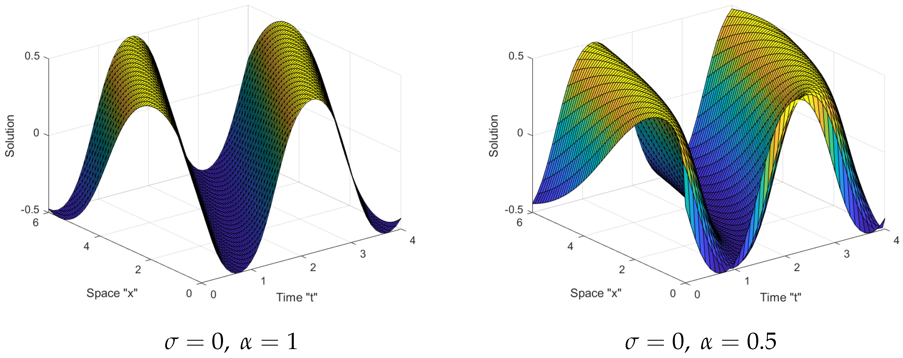
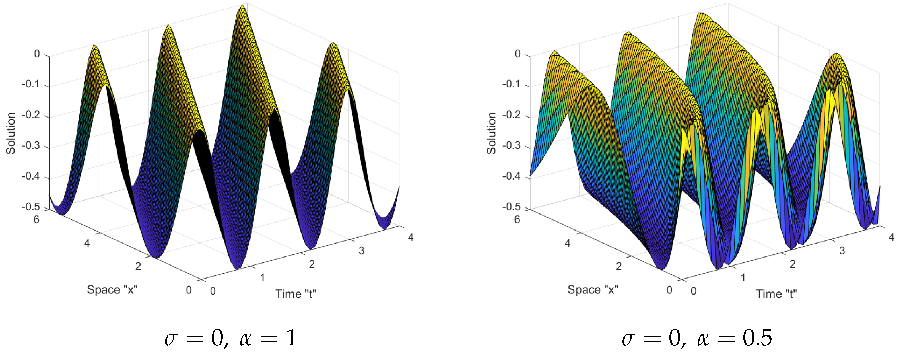
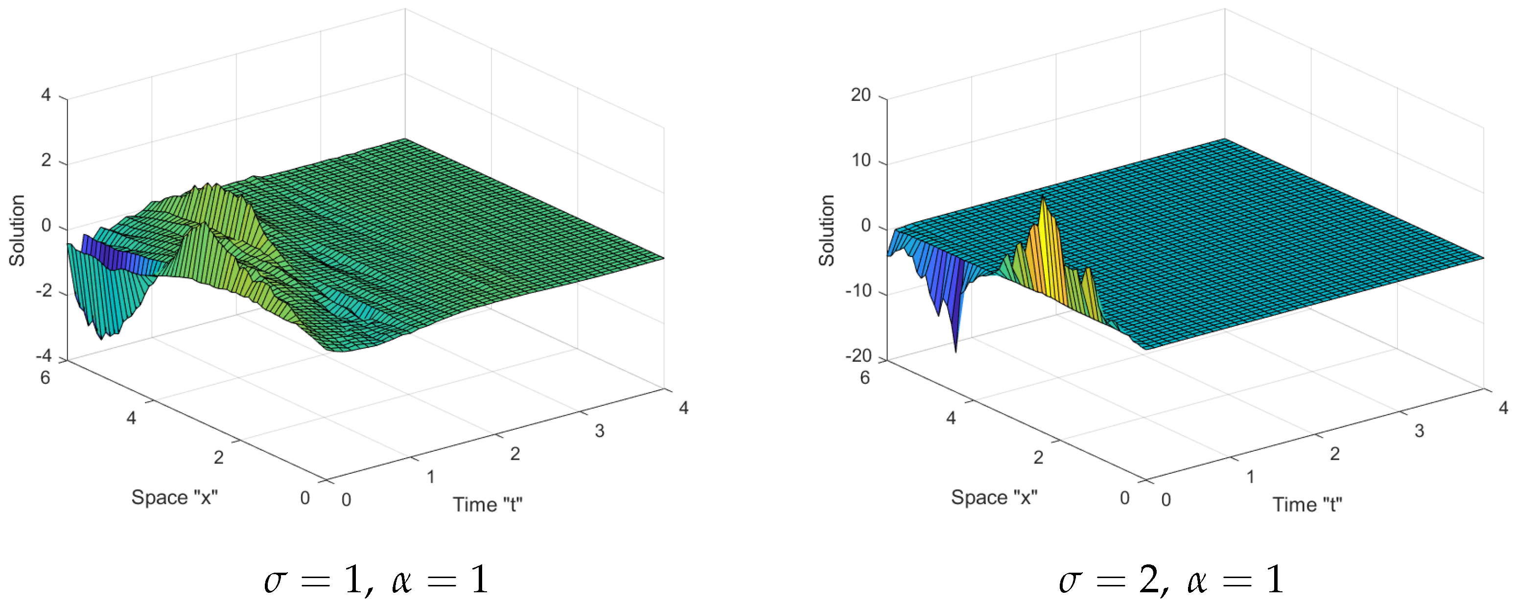
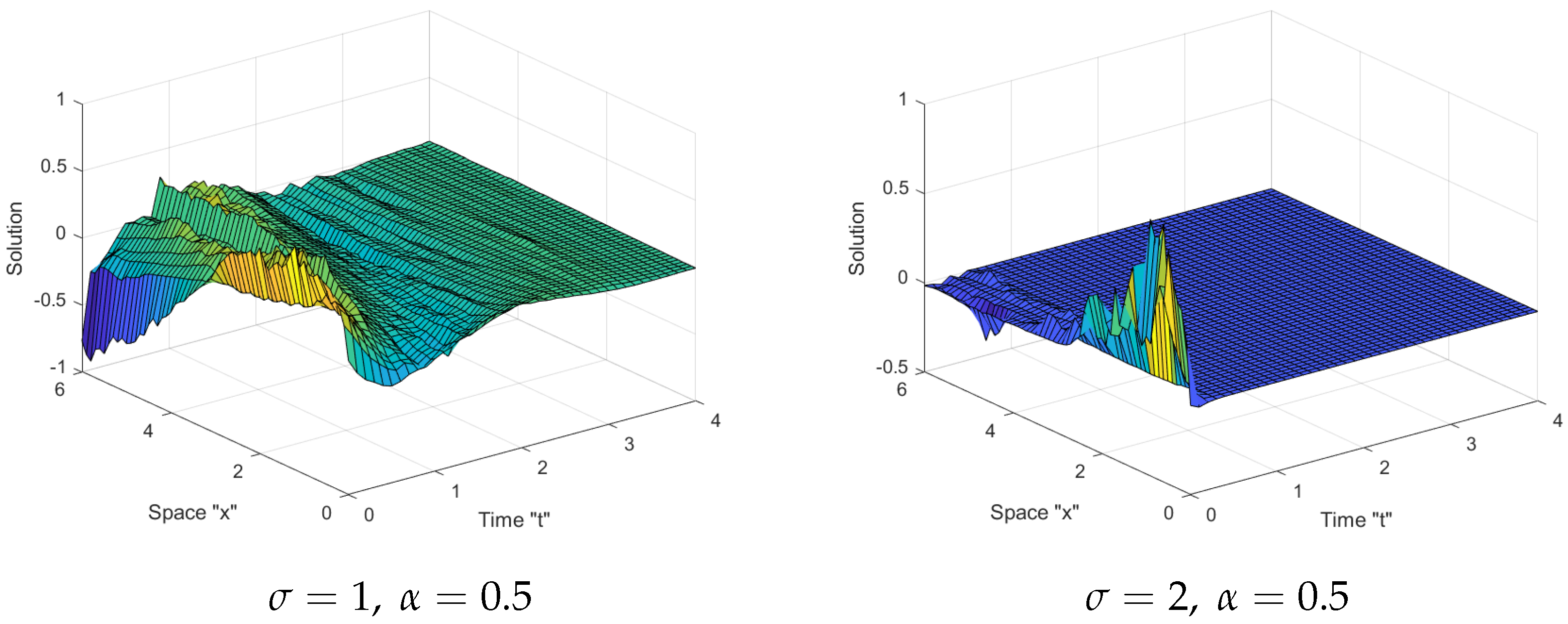
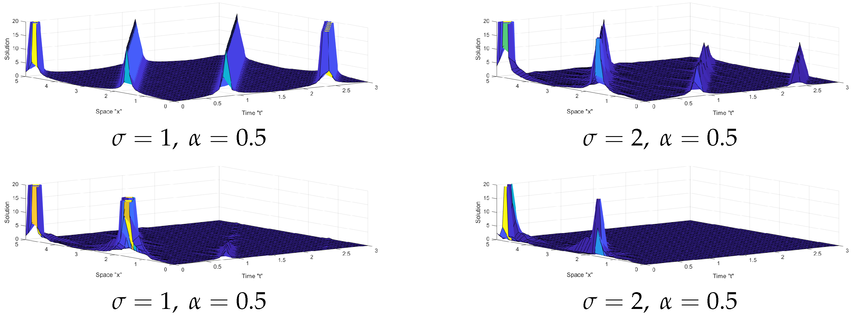
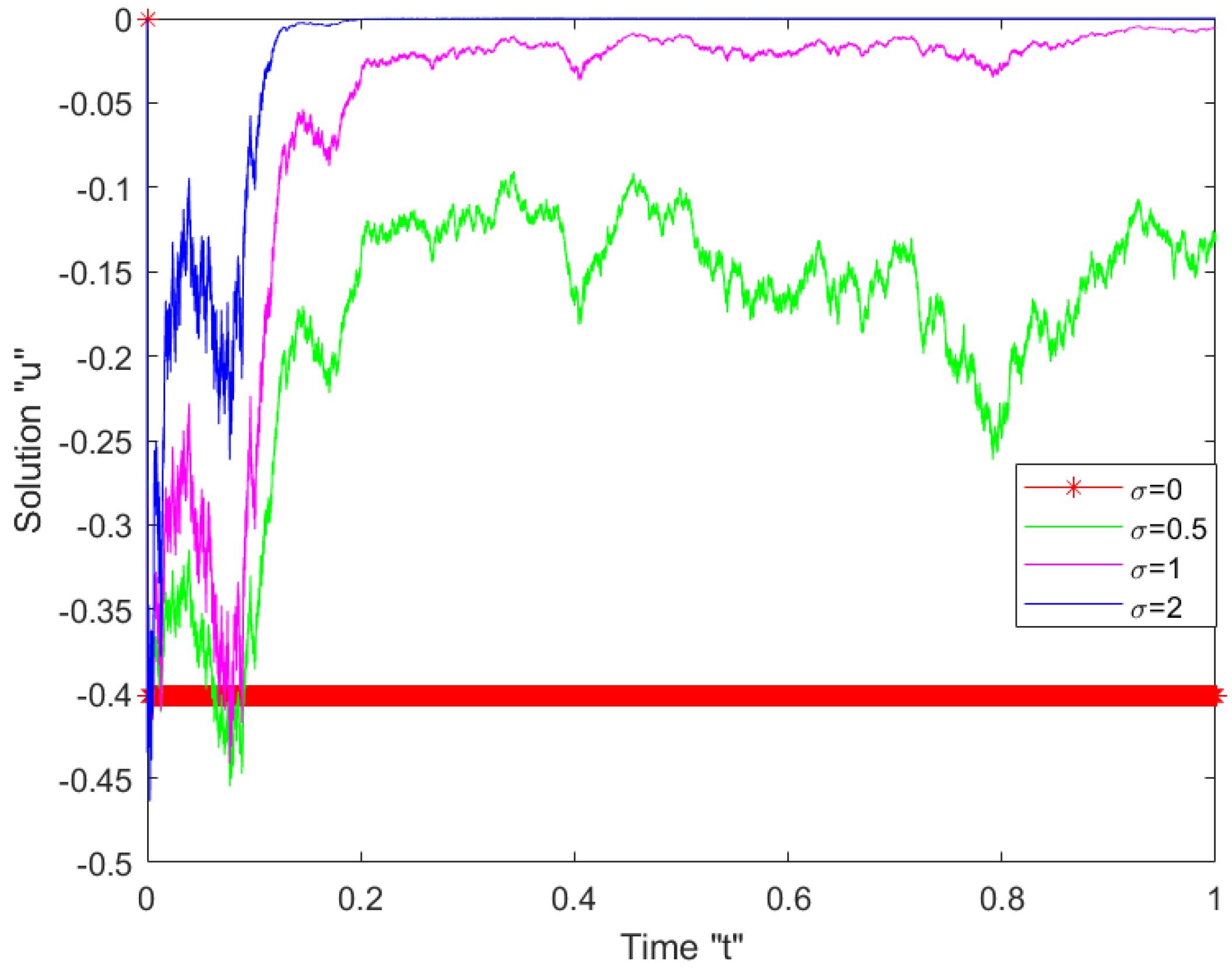
5. The Influence of Noise on SFSZS Solutions

The influence of the noise on the analytical solution of the SFSZS (2)–(3) is addressed here. Fix the parameters k = 1 , ρ = 1 , m = 0.5 , and λ = 3 . We introduce a number of simulations for various values of σ (noise intensity) and α (fractional derivative order). We employ the MATLAB tools to plot our figures. In Figure 1 and Figure 2, if σ = 0 , we see that the surface fluctuates for different values of α :
In the following Figure 3, Figure 4 and Figure 5, we can see that after minor transit patterns, the surface becomes considerably flattered when noise is included and its strength is increased σ = 1 , 2 .
In Figure 6, we introduce 2D plots of the u in (31) with σ = 0 , 0.5 , 1 , 2 and α = 1 , which emphasize the results above.
From Figure 1, Figure 2, Figure 3, Figure 4, Figure 5 and Figure 6, we deduce the following:
  • The surface expands as the fractional order α increases;
  • Multiplicative Wiener process stabilizes the solutions of SFSBE around zero.

6. Conclusions

In this article, we provided a wide range of exact solutions of the stochastic fractional Zakharov system (2)–(3). We applied two different methods such as the Riccati–Bernoulli sub-ODE method and Jacobi elliptic function method to attain rational, trigonometric, hyperbolic, and elliptic stochastic fractional solutions. Such solutions are critical for comprehending certain essential, fundamental, complex phenomena. The solutions obtained will be extremely useful for further studies such as fiber applications, spatial plasma, quasi particle theory, coastal water motion, and industrial research. Finally, the effect of multiplicative Wiener process on the exact solution of Zakharov system (2)–(3) is demonstrated. In future research, we can address the fractional-time Zakharov system (2)–(3) with multidimensional multiplicative noise.

Author Contributions

Conceptualization, F.M.A.-A., W.W.M., M.A. and M.E.-M.; methodology, F.M.A.-A. and W.W.M.; software, W.W.M. and M.E.-M.; formal analysis, F.M.A.-A., W.W.M., M.A. and M.E.-M.; investigation, F.M.A.-A. and W.W.M.; resources, F.M.A.-A., W.W.M., M.A. and M.E.-M.; data curation, F.M.A.-A. and W.W.M.; writing—original draft preparation, F.M.A.-A., W.W.M., M.A. and M.E.-M.; writing—review and editing, F.M.A.-A. and W.W.M.; visualization, F.M.A.-A. and W.W.M. All authors have read and agreed to the published version of the manuscript.

Funding

This research received no external funding.

Institutional Review Board Statement

Not applicable.

Informed Consent Statement

Not applicable.

Data Availability Statement

Not applicable.

Acknowledgments

Princess Nourah bint Abdulrahman University Researchers Supporting Project number (PNURSP2022R273), Princess Nourah bint Abdulrahman University, Riyadh, Saudi Arabia.

Conflicts of Interest

The authors declare no conflict of interest.

References

  1. Zakharov, V.E. Collapse of Langmuir waves. Sov. J. Exper. Theor. Phys. 1972, 35, 908–914. [Google Scholar]
  2. Goubet, O.; Moise, I. Attractors for dissipative Zakharov equations. Nonlinear Anal. TMA 1998, 31, 823–847. [Google Scholar] [CrossRef]
  3. Guo, B. On the IBVP for some more extensive Zakharov equations. J. Math. 1987, 7, 269–275. [Google Scholar]
  4. Li, Y. On the initial boundary value problems for two dimensional systems of Zakharov equations and of complex-Schrödinger-real-Boussinesq equations. J. Partial Diff. Equ. 1992, 5, 81–93. [Google Scholar]
  5. Masselin, V. A result on the blow-up rate for the Zakharov equations in dimension 3. SIAM J. Math. Anal. 2001, 33, 440–447. [Google Scholar] [CrossRef]
  6. Guo, B.; Sheng, L. The global existence and uniqueness of classical solutions of periodic initial boundary problems of Zakharov equations. Acta Math. Appl. Sin. 1982, 5, 310–324. [Google Scholar]
  7. Song, M.; Liu, Z. Traveling wave solutions for the generalized Zakharov equations. Math. Probl. Eng. 2012, 2012, 747295. [Google Scholar] [CrossRef]
  8. Wang, M.L.; Li, X.Z. Extended F-expansion method and periodic wave solutions for the generalized Zakharov equations. Phys. Lett. A 2005, 343, 48–54. [Google Scholar] [CrossRef]
  9. Javidi, M.; Golbabai, A. Construction of a solitary wave solution for the generalized Zakharov equation by a variational iteration method. Comput. Math. Appl. 2007, 54, 1003–1009. [Google Scholar] [CrossRef] [Green Version]
  10. Taghizadeh, N.; Mirzaadsh, M.; Farahrooz, F. Exact solutions of the generalized-Zakharov (GZ) equation by the infinite series method. Appl. Appl. Math. 2010, 5, 621–628. [Google Scholar]
  11. Hong, B.; Lu, D.; Sun, F. The extended Jacobi Elliptic Functions expansion method and new exact solutions for the Zakharov equations. World J. Model. Simul. 2009, 5, 216–224. [Google Scholar]
  12. Yuste, S.B.; Acedo, L.; Lindenberg, K. Reaction front in an A + BC reaction–subdiffusion process. Phys. Rev. E 2004, 69, 036126. [Google Scholar] [CrossRef] [Green Version]
  13. Mohammed, W.W.; Iqbal, N. Impact of the same degenerate additive noise on a coupled system of fractional space diffusion equations. Fractals 2022, 30, 2240033. [Google Scholar] [CrossRef]
  14. Iqbal, N.; Yasmin, H.; Ali, A.; Bariq, A.; Al-Sawalha, M.M.; Mohammed, W.W. Numerical Methods for Fractional-Order Fornberg-Whitham Equations in the Sense of Atangana-Baleanu Derivative. J. Funct. Spaces 2021, 2021, 2197247. [Google Scholar] [CrossRef]
  15. Mohammed, W.W. Approximate solutions for stochastic time-fractional reaction–diffusion equations with multiplicative noise. Math. Methods Appl. Sci. 2021, 44, 2140–2157. [Google Scholar] [CrossRef]
  16. Iqbal, N.; Wu, R.; Mohammed, W.W. Pattern formation induced by fractional cross-diffusion in a 3-species food chain model with harvesting. Math. Comput. Simul. 2021, 188, 102–119. [Google Scholar] [CrossRef]
  17. Barkai, E.; Metzler, R.; Klafter, J. From continuous time random walks to the fractional Fokker–Planck equation. Phys. Rev. 2000, 61, 132–138. [Google Scholar] [CrossRef]
  18. Arnold, L. Random Dynamical Systems; Springer: Berlin, Germany, 1998. [Google Scholar]
  19. Weinan, E.; Li, X.; Vanden-Eijnden, E. Some Recent Progress in Multiscale Modeling, Multiscale Modeling and Simulation; Lect. Notes in Computer Science Engineering; Springer: Berlin, Germany, 2004; Volume 39, pp. 3–21. [Google Scholar]
  20. Mohammed, W.W.; Blömker, D. Fast diffusion limit for reaction-diffusion systems with stochastic Neumann boundary conditions. SIAM J. Math. Anal. 2016, 48, 3547–3578. [Google Scholar] [CrossRef] [Green Version]
  21. Mohammed, W.W. Modulation Equation for the Stochastic Swift–Hohenberg Equation with Cubic and Quintic Nonlinearities on the Real Line. Mathematics 2020, 6, 1217. [Google Scholar] [CrossRef] [Green Version]
  22. Khalil, R.; Al Horani, M.; Yousef, A.; Sababheh, M. A new definition of fractional derivative. J. Comput. Appl. Math. 2014, 264, 65–70. [Google Scholar] [CrossRef]
  23. Guo, B.; Lv, Y.; Yang, X. Dynamics of Stochastic Zakharov Equations. J. Math. Phys. 2009, 50, 052703. [Google Scholar] [CrossRef]
  24. Guo, Y.; Guo, B.; Li, D. Global random attractors for the stochastic dissipative Zakharov equations. Acta Math. Appl. Sin. 2014, 30, 289–304. [Google Scholar] [CrossRef]
  25. Guo, Y.F.G.B.; Li, D. Asymptotic behavior of stochastic dissipative quantum Zakharov equations. Stoch. Dyn. 2013, 13, 1250016. [Google Scholar] [CrossRef]
  26. Kloeden, P.E.; Platen, E. Numerical Solution of Stochastic Differential Equations; Springer: New York, NY, USA, 1995. [Google Scholar]
  27. Yang, X.F.; Deng, Z.C.; Wei, Y. A Riccati-Bernoulli sub-ODE method for nonlinear partial differential equations and its application. Adv. Diff. Equ. 2015, 1, 117–133. [Google Scholar] [CrossRef] [Green Version]
  28. Fan, E.; Zhang, J. Applications of the Jacobi elliptic function method to special-type nonlinear equations. Phys. Lett. A 2002, 305, 383–392. [Google Scholar] [CrossRef]
Figure 1. 3D graphs of the solution (31).
Mathematics 10 01194 g001
Figure 2. 3D graphs of the solution (32).
Mathematics 10 01194 g002
Figure 3. 3D graphs of the solution (31) with α = 1 .
Mathematics 10 01194 g003
Figure 4. 3D graphs of the equation (31) with α = 0.5 .
Mathematics 10 01194 g004
Figure 5. 3D graphs of the equation (21) with α = 1 .
Mathematics 10 01194 g005
Figure 6. 2D graphs of the u in (31).
Mathematics 10 01194 g006
Publisher’s Note: MDPI stays neutral with regard to jurisdictional claims in published maps and institutional affiliations.

