Adaptive Neural Network Sliding Mode Control for a Class of SISO Nonlinear Systems

Abstract

In this article, a sliding mode control (SMC) is proposed on the basis of an adaptive neural network (NN) for a class of Single-Input–Single-Output (SISO) nonlinear systems containing unknown dynamic functions. Since the control objective is to steer the system states to track the given reference signals, the SMC method is considered by employing the adaptive neural network (NN) strategy for dealing with the unknown dynamic problem. In order to compress the impaction coming from chattering phenomenon (which inherently exists in most SMC methods because of the discontinuous switching term), the boundary layer technique is considered. The basic design idea is to introduce a continuous proportional function to replace the discontinuous switching control term inside the boundary layer so that the chattering can be effectively alleviated. Finally, both Lyapunov theoretical analysis and computer numerical simulation are used to verify the effectiveness of the proposed SMC method.

1. Introduction

In the past decades, owing to the rapid development of industry, scientists have increasingly used nonlinear control because it is applied for practical engineering systems more effectively, such as for aircraft flight control systems [1], power systems [2] and hydraulic robot manipulator control systems [3].

To achieve nonlinear system control, sliding mode control (SMC) has always been one of the popular strategies due to the advantages of rapid global convergence, simple structure, low sensitivity for parameter variations and high robustness for external disturbances. Its basic idea is to force and constrain the systems states to lie within the neighborhood of prescribed sliding surface. In order to define or design the sliding surface, there are many different methods are suggested, such as the controllable canonical form method [4], the Filippov theory [5,6] and the equivalent control method [7].

Among them, the equivalent control method is a straightforward technique coming from the Filippov theory. With the development of control theory, sliding mode strategy has been widely extended to different fields [8,9,10,11,12] and has become a favorite control means for industrial applications, such as mechanical systems [13], robot manipulators [14] and electric drives [15]. Specifically, it is also studied for nonlinear systems under unknown dynamics [16,17,18].

In most published nonlinear control methods, there is a common assumption that the dynamic function is known or Lipschitz continuous; however, the real-world engineering system ubiquitously works in complicated and volatile dynamic environments and cannot acquire accurate system modeling acknowledge. It has been proven that neural networks (NNs) or fuzzy logic systems (FLSs) can approximate unknown continuous functions to any desired accuracy. By taking advantage of the highlighting property, a great number of nonlinear control methods have been studied in the literature [19,20,21,22,23,24]. Recently, many adaptive sliding mode tracking controls combined with NNs have been reported because NNs can compensate for the system uncertainties and has received considerable attention, including [25,26,27,28].

It is worth mentioning that the SMC is often accompanied by the chattering phenomenon, which is caused from the discontinuous switching control signal [29,30,31]. This phenomenon can seriously affect the system performance or even lead to instability [32]. To handle the problem, many popular methods have been proposed, such as replacing the discontinuous control law with a saturation function [33], integral sliding mode control method [34], terminal sliding mode control method [35], PI sliding mode control method [36], PID sliding mode control method [37] and boundary layer control technique [38].

Among them, the boundary layer approach is widespread thanks to its simple design and outstanding performance. As the discontinuous switching control term is replaced by a continuous proportional function inside the boundary layer, the chattering phenomenon is significantly alleviated. However, in most articles, the continuous function is selected to be the PI form function or PID form function, and unfortunately they are difficult to implement and apply.

Being motivated by the above analysis, for an unknown dynamic high-order SISO nonlinear system, we design an NN approximation based adaptive SMC for steering the system states to follow the reference signals. To alleviate the chattering phenomenon, a simple proportional function is designed to replace the discontinuous control inside the introduced boundary layer. For demonstrating the effectiveness of the proposed method, a numerical simulation example is performed to show the desired results. The main contributions are summarized in the following:

(i)

The proposed SMC control can effectively compensate the unknown dynamic. Since the adaptive NN strategy is integrated in the control design, the proposed nonlinear SMC control can avoid requiring accurate dynamic acknowledge.

(ii)

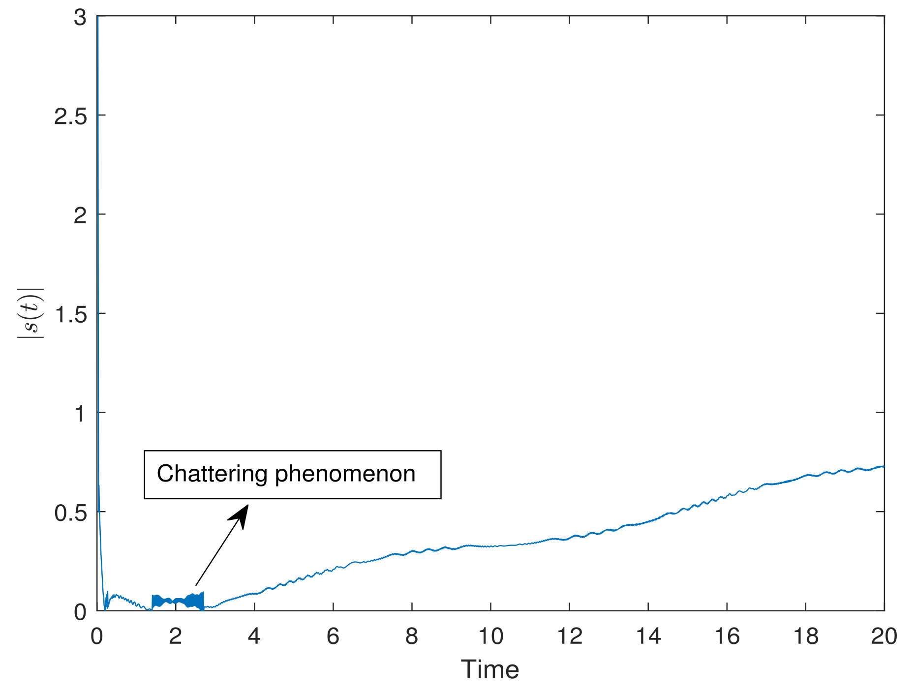
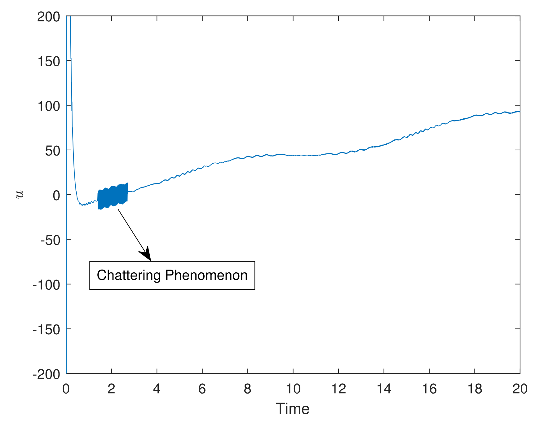
The proposed SMC control can effectively alleviate the chattering problem by using the boundary layer. Since this method is to use the continuous proportional function to replace the discontinuous switching control, it can be more easily implemented.

2. Problem Statement

Consider the following nth-order nonlinear Single-Input–Single-Output (SISO) dynamic system modeled in the controllability canonical form:

$$\left\{\begin{array}{ccc}\hfill {\dot{\chi }}_1\left(t\right)& =& {\chi }_2\left(t\right),\hfill \\ \hfill {\dot{\chi }}_2\left(t\right)& =& {\chi }_3\left(t\right),\hfill \\ \hfill & \cdots & \\ \hfill {\dot{\chi }}_n\left(t\right)& =& f\left(\overline{\chi }\right)+u,\hfill \end{array}\right.$$

(1)

where $\overline{\chi }\left(t\right)={[{\chi }_1\left(t\right),{\chi }_2\left(t\right),\cdots ,{\chi }_n\left(t\right)]}^T={[{\chi }_1,\dot{{\chi }_1},\cdots ,{\chi }_1^{(n-1)}]}^T\in R^n$ is the state vector, $u\in R$ is the control input variable and $f\left(\overline{\chi }\right)\in R$ is the unknown smooth nonlinear dynamic function.

Definition 1 (Semi-Globally Uniformly Ultimately Bounded (SGUUB)).

The solution of (1) is SGUUB, if $\forall \overline{\chi }\left(t_0\right)={\overline{\chi }}_0\in \Omega$ where $\Omega$ is a compact subset of $R^n$, there exists two positive constants $\rho$ and $T(\rho ,{\overline{\chi }}_0)$ such that $\parallel \overline{\chi }\left(t\right)\parallel <\rho$ for $\forall t>t_0+T$.

Control Objective. The control objective is to design an adaptive NN sliding mode controller for system (1), such that all control signals of the closed-loop control are SGUUB. The system state $\overline{\chi }$ can follow the desired reference trajectory ${\overline{\chi }}_d\left(t\right)={[{\chi }_{d1}\left(t\right),{\chi }_{d2}\left(t\right),\cdots ,{\chi }_{dn}\left(t\right)]}^T$$={[{\chi }_d,{\dot{\chi }}_d,\cdots ,{\chi }_d^{(n-1)}]}^T\in R^n$, which can be exactly measured.

The tracking error vector $\xi \left(t\right)$$\in R^n$ is defined as

$$\begin{array}{cc}\hfill \xi \left(t\right)=& {[{\xi }_1\left(t\right),{\xi }_2\left(t\right),\cdots ,{\xi }_n\left(t\right)]}^T\hfill \\ \hfill =& \overline{\chi }\left(t\right)-{\overline{\chi }}_d\left(t\right)\hfill \\ \hfill =& {[{\chi }_1\left(t\right)-{\chi }_{d1}\left(t\right),{\chi }_2\left(t\right)-{\chi }_{d2}\left(t\right),\cdots ,{\chi }_n\left(t\right)-{\chi }_{dn}\left(t\right)]}^T\hfill \end{array}$$

(2)

Furthermore, the sliding variable $s\left(t\right)\in R$ is constructed as

$$\begin{array}{cc}\hfill s\left(t\right)=& c_1{\xi }_1\left(t\right)+c_2{\dot{\xi }}_1\left(t\right)+\cdots +c_{n-1}{\xi }_1^{(n-2)}\left(t\right)+{\xi }_1^{(n-1)}\left(t\right)\hfill \\ \hfill =& c_1{\xi }_1\left(t\right)+c_2{\xi }_2\left(t\right)+\cdots +c_{n-1}{\xi }_{n-1}\left(t\right)+{\xi }_n\left(t\right)\hfill \\ \hfill =& \sum _{i=1}^{n-1}{c}_i{\xi }_i\left(t\right)+{\xi }_n\left(t\right),\hfill \end{array}$$

(3)

where these coefficients $c_1,c_2,\cdots ,c_{n-1}$ are selected to make the polynomial $h\left(\lambda \right)={\lambda }^{n-1}+c_{n-1}{\lambda }^{n-2}+\cdots +c_1$ to be Hurwitz, i.e., all the eigenvalues are in the open left half-plane, and $\lambda$ is the Laplace operator.

In terms of (1), the sliding dynamic can be yielded as

$$\begin{array}{cc}\hfill \dot{s}\left(t\right)=& c_1{\dot{\xi }}_1\left(t\right)+c_2{\dot{\xi }}_2\left(t\right)+\cdots +c_{n-1}{\dot{\xi }}_{n-1}\left(t\right)+{\dot{\xi }}_n\left(t\right)\hfill \\ \hfill =& \sum _{i=1}^{n-1}{c}_i{\xi }_{i+1}\left(t\right)-{\chi }_{dn}\left(t\right)+f\left(\overline{\chi }\right)+u.\hfill \end{array}$$

(4)

According to the sliding control mechanism, the control task can be accomplished by finding the adaptive NN sliding mode control law to steer the dynamic system (1) to keep on the sliding surface $s\left(t\right)=0$.

For reaching the sliding surface $s\left(t\right)=0$, a sufficient condition is

$$\begin{array}{c}\hfill \frac{1}{2}\frac{d{s}^2\left(t\right)}{dt}\le -\eta \left|s\left(t\right)\right|,\eta >0,\end{array}$$

(5)

where $\eta$ is a constant [39].

To meet the sufficient condition (5), the SMC u will be designed to contain two basic control terms, which are the continuous equivalent control term $u_{eq}$ and the discontinuous switching control term $u_{sw}$ formulated as

$$\begin{array}{cc}\hfill u_{eq}=& -\sum _{i=1}^{n-1}{c}_i{\xi }_{i+1}\left(t\right)+{\chi }_{dn}\left(t\right)-f\left(\overline{\chi }\right),\hfill \\ \hfill u_{sw}=& -k_{p}s\left(t\right)-{\eta }_{sw}sgn\left(s\right),\hfill \end{array}$$

(6)

where $k_{p}s\left(t\right)$ is the high-gain proportional function with $k_p>0$, ${\eta }_{sw}\ge \eta >0$ is a positive constant, and $sgn\left(s\right)$ is the sign function as

$$sgn\left(s\right)=\left\{\begin{array}{ccc}\hfill 1,& & fors>0,\hfill \\ \hfill 0,& & fors=0,\hfill \\ \hfill -1,& & fors<0.\hfill \end{array}\right.$$

(7)

Remark 1.

With respect to the switching control term $u_{sw}$, if we choose a greater parameter ${\eta }_{sw}$, it will yield a faster convergence rate. However, this will also cause a high scale chattering phenomenon. Hence, it is difficult to balance convergence rate and the magnitude of chattering.

Consequently, the SMC law can be obtained as

$$\begin{array}{cc}\hfill u=& u_{eq}+u_{sw},\hfill \\ \hfill =& -\sum _{i=1}^{n-1}{c}_i{\xi }_{i+1}\left(t\right)+{\chi }_{dn}\left(t\right)-f\left(\overline{\chi }\right)-k_{p}s\left(t\right)-{\eta }_{sw}sgn\left(s\right).\hfill \end{array}$$

(8)

In order to verify effectiveness of the control law, consider the following Lyapunov function candidate as

$$\begin{array}{c}\hfill V_1\left(t\right)=\frac{1}{2}{s}^2\left(t\right)\end{array}$$

(9)

Calculate the first derivative of (9) along (4) and implement (8) to have

$$\begin{array}{cc}\hfill {\dot{V}}_1\left(t\right)=& s\left(t\right)\dot{s}\left(t\right)\hfill \\ \hfill =& s\left(t\right)\left(\sum _{i=1}^{n-1}{c}_i{\xi }_{i+1}\left(t\right)+f\left(\overline{\chi }\right)+u-{\chi }_{dn}\left(t\right)\right)\hfill \\ \hfill =& -k_p{s}^2\left(t\right)-{\eta }_{sw}s\left(t\right)sgn\left(s\right)\hfill \\ \hfill \le & -{\eta }_{sw}\left|s\left(t\right)\right|\le -\eta \left|s\left(t\right)\right|.\hfill \end{array}$$

(10)

The above inequality (10) implies that the SMC (8) can meet the sufficient condition (5). Then, tracking error variable $\xi \left(t\right)$ will converge exponentially to the desired equilibrium point.

3. Main Results

However, the function $f\left(\overline{\chi }\right)$ is often unknown in practical engineering, and thus the control law (8) is unavailable. To solve the problem, the unknown continuous function $f\left(\overline{\chi }\right)$ will be approximated by using the adaptive NN technology in the following form.

$$\begin{array}{cc}\hfill f\left(\overline{\chi }\right)=& {\omega }_f^{*T}{\Psi }_f\left(\overline{\chi }\right)+{ϵ}_f.\hfill \end{array}$$

(11)

where ${\omega }_f^{*}\in R^{q\times m}$ is the ideal NN weight matrix, and q is the neuron number, ${\Psi }_f\left(\overline{\chi }\right)\in R^q$ is the Gaussian activation function vector, and ${ϵ}_f\in R^m$ is the bounded approximation error (the detailed introduction concerning NN approximation in [40]).

Using the NN approximation (11), the SMC (8) becomes

$$\begin{array}{c}\hfill u=-\sum _{i=1}^{n-1}{c}_i{\xi }_{i+1}\left(t\right)+{\chi }_{dn}\left(t\right)-({\omega }_f^{*T}{\Psi }_f\left(\overline{\chi }\right)+{ϵ}_f)-k_{p}s\left(t\right)-{\eta }_{sw}sgn\left(s\right).\end{array}$$

(12)

It should be mentioned that the ideal weight ${\omega }_f^{*}$ is an unknown constant matrix, and thus the NN-based SMC (12) is invalid in the actual control. To derive the available NN controller, we need to replace the unknown constant weight ${\omega }_f^{*}$ via using its adaptive estimation ${\widehat{\omega }}_f\left(t\right)$. Then, the sliding mode control (8) can become the following form as

$$\begin{array}{cc}\hfill u=& -\sum _{i=1}^{n-1}{c}_i{\xi }_{i+1}\left(t\right)+{\chi }_{dn}\left(t\right)-{\widehat{\omega }}_f^T\left(t\right){\Psi }_f\left(\overline{\chi }\right)-k_{p}s\left(t\right)-{\eta }_{sw}sgn\left(s\right).\hfill \end{array}$$

(13)

The NN weight ${\widehat{\omega }}_f\left(t\right)$ is trained by the following adaptive updating law,

$$\begin{array}{cc}\hfill {\dot{\widehat{\omega }}}_f\left(t\right)=& {\kappa }_f\left({\Psi }_f\left(\overline{\chi }\right)s\left(t\right)-{\sigma }_f{\widehat{\omega }}_f\left(t\right)\right)\hfill \end{array}$$

(14)

where ${\kappa }_f$ is a positive proportional coefficient for the NN’s learning speed, ${\sigma }_f$ is a positive constant for the system robustness [41].

However, due to the existence of the discontinuous sign function in (13), the high frequency chattering will be caused around the sliding surface. To deal with this problem, the boundary layer method is adopted by introducing a thickness $\Phi$ [42]. In order to execute the boundary lay method, the switching control term $u_{sw}$ is redesigned according to the following situation.

When the sliding variable $s\left(t\right)$ is outside the boundary layer, i.e., $\left|s\right(t\left)\right|\ge \Phi$, the control (13) is retained, where the discontinuous sign function $-{\eta }_{sw}sgn\left(s\right)$ aims for fast convergence speed. When the sliding variable $s\left(t\right)$ is inside the boundary layer, i.e., $\left|s\right(t\left)\right|<\Phi$, the control (13) is switched to the situation that only the high-gain proportional function $-k_{p}s\left(t\right)$ is kept and the discontinuous sign function $-{\eta }_{sw}sgn\left(s\right)$ is removed for alleviating the chattering phenomenon.

Thus, we can obtain the following actual control law for system (1)

$$\begin{array}{c}\hfill u=-\sum _{i=1}^{n-1}{c}_i{\xi }_{i+1}\left(t\right)+{\chi }_{dn}\left(t\right)-{\widehat{\omega }}_f^T\left(t\right){\Psi }_f\left(\overline{\chi }\right)+u_{sw},\end{array}$$

(15)

where

$$u_{sw}=\left\{\begin{array}{ccc}\hfill & -k_{p}s\left(t\right)-{\eta }_{sw}sgn\left(s\right),& \left|s\right(t\left)\right|\ge \Phi ,\hfill \\ \hfill & -k_{p}s\left(t\right),& \left|s\right(t\left)\right|<\Phi .\hfill \end{array}\right.$$

(16)

Remark 2.

According to the definition (16) of the switching control term, it can be easily concluded that the control (15) is only continuous or $C_1$ continuous inside the boundary layer. However, in the outside of boundary layer, the control (15) is discontinuous because the switching term $u_{sw}$ involves the sign function $sgn\left(s\right)$. Although the discontinuity may cause the controller oscillation, it can achieve a fast convergence rate.

4. Stability Analysis

Lemma 1

([43]). The positive continuous function $V\left(t\right)\in \mathbb{R}$ is with the bounded initial value $V\left(0\right)$. If it meets $\dot{V}\left(t\right)\le -pV\left(t\right)+q$, where $p>0$ and $q>0$, then it will also satisfy the following inequality,

$$\begin{array}{c}\hfill V\left(t\right)\le V\left(0\right)e^{-pt}+\frac{q}{p}\left(1-e^{-pt}\right).\end{array}$$

(17)

Theorem 1.

Consider the class of SISO nonlinear systems (1). If the adaptive sliding control (15) with the NN updating law (14) is performed, and appropriate design constants are selected, then the following control objectives can be achieved.

( 1 )

All error signals$\xi \left(t\right)$,${\tilde{\omega }}_f\left(t\right)$of the closed loop control are SGUUB.

( 2 )

The tracking error$\xi \left(t\right)$converges to a small neighborhood of zero.

Proof. 

Select the Lyapunov function candidate as

$$\begin{array}{c}\hfill V_2\left(t\right)=\frac{1}{2}{s}^2\left(t\right)+\frac{1}{2{\kappa }_f}{\tilde{\omega }}_f^T\left(t\right){\tilde{\omega }}_f\left(t\right),\end{array}$$

(18)

where ${\tilde{\omega }}_f\left(t\right)={\widehat{\omega }}_f\left(t\right)-{\omega }_f^{*}$.

Calculate the time derivative of $V_2\left(t\right)$ along (4) and (14) as

$$\begin{array}{cc}\hfill {\dot{V}}_2\left(t\right)=& s\left(t\right)\dot{s}\left(t\right)+\frac{1}{{\kappa }_f}{\tilde{\omega }}_f^T\left(t\right){\dot{\widehat{\omega }}}_f\left(t\right)\hfill \\ \hfill =& s\left(t\right)\left(\sum _{i=1}^{n-1}{c}_i{\xi }_{i+1}\left(t\right)+f\left(\overline{\chi }\right)+u-{\chi }_{dn}\left(t\right)\right)\hfill \\ \hfill & +{\tilde{\omega }}_f^T\left(t\right)\left({\Psi }_f\left(\overline{\chi }\right)s\left(t\right)-{\sigma }_f{\widehat{\omega }}_f\left(t\right)\right).\hfill \end{array}$$

(19)

Substituting (11) and (15) into the above Equation (19) results in

$$\begin{array}{cc}\hfill {\dot{V}}_2\left(t\right)=& s\left(t\right)\left(-{\tilde{\omega }}_f^T\left(t\right){\Psi }_f\left(\overline{\chi }\right)+u_{sw}+{ϵ}_f\right)\hfill \\ \hfill & +{\tilde{\omega }}_f^T\left(t\right)\left({\Psi }_f\left(\overline{\chi }\right)s\left(t\right)-{\sigma }_f{\widehat{\omega }}_f\left(t\right)\right).\hfill \end{array}$$

(20)

After several simple mathematical operations, the above Equation (20) can be transformed as

$$\begin{array}{cc}\hfill {\dot{V}}_2\left(t\right)=& s\left(t\right)u_{sw}+s\left(t\right){ϵ}_f-{\sigma }_f{\tilde{\omega }}_f^T\left(t\right){\widehat{\omega }}_f\left(t\right).\hfill \end{array}$$

(21)

Using the fact ${\tilde{\omega }}_f\left(t\right)={\widehat{\omega }}_f\left(t\right)-{\omega }_f^{*}$, there is the following equation,

$$\begin{array}{cc}\hfill {\tilde{\omega }}_f^T\left(t\right){\widehat{\omega }}_f\left(t\right)=& \frac{1}{2}{\tilde{\omega }}_f^T\left(t\right){\tilde{\omega }}_f\left(t\right)+\frac{1}{2}{\widehat{\omega }}_f^T\left(t\right){\widehat{\omega }}_f\left(t\right)-\frac{1}{2}{\omega }_f^{*T}{\omega }_f^{*},\hfill \end{array}$$

(22)

Substituting (22) into (21), it can be rewritten as

$$\begin{array}{cc}\hfill {\dot{V}}_2\left(t\right)\le & s\left(t\right)u_{sw}+s\left(t\right){ϵ}_f-\frac{{\sigma }_f}{2}{\tilde{\omega }}_f^T\left(t\right){\tilde{\omega }}_f\left(t\right)+\frac{{\sigma }_f}{2}{\omega }_f^{*T}{\omega }_f^{*}.\hfill \end{array}$$

(23)

Next, the system stability will be analyzed for two situations corresponding to (16), i.e., $\left|s\right|\ge \Phi$ and $\left|s\right|<\Phi$.

(1) For the condition $\left|s\right|\ge \Phi$, the sliding variable is outside the boundary layer. According to (16), the switching control part $u_{sw}$ is selected as $u_{sw}=-\left(k_{p}s\left(t\right)+{\eta }_{sw}sgn\left(s\right)\right)$. Inserting it into (23) leads to

$$\begin{array}{c}\hfill {\dot{V}}_2\left(t\right)\le -k_p{s}^2\left(t\right)-{\eta }_{sw}\left|s\left(t\right)\right|+s\left(t\right){ϵ}_f-\frac{{\sigma }_f}{2}{\tilde{\omega }}_f^T\left(t\right){\tilde{\omega }}_f\left(t\right)+\frac{{\sigma }_f}{2}{\omega }_f^{*T}{\omega }_f^{*}.\end{array}$$

(24)

Using the fact $s\left(t\right){ϵ}_f\le \frac{1}{2}{s}^2\left(t\right)+\frac{1}{2}{ϵ}_f^2$, the above inequality (24) can become the following one

$$\begin{array}{cc}\hfill {\dot{V}}_2\left(t\right)\le & -\left(k_p-\frac{1}{2}\right)s^2\left(t\right)-{\eta }_{sw}\left|s\left(t\right)\right|-\frac{{\sigma }_f}{2}{\tilde{\omega }}_f^T\left(t\right){\tilde{\omega }}_f\left(t\right)+\tau \left(t\right)\hfill \\ \hfill \le & -\left(k_p-\frac{1}{2}\right)s^2\left(t\right)-{\eta }_{sw}\left|s\left(t\right)\right|+\beta ,\hfill \end{array}$$

(25)

where $\tau \left(t\right)=\frac{1}{2}{ϵ}_f^2+\frac{{\sigma }_f}{2}{\omega }_f^{*T}{\omega }_f^{*}$ that is bounded by a constant $\beta$, i.e., $\tau \left(t\right)\le \beta$.

Through selecting the designed constant satisfies ${\eta }_{sw}\ge \frac{\beta }{\Phi }$ and $k_p\ge \frac{\beta }{{\Phi }^2}+\frac{1}{2}$, we can ensure ${\dot{V}}_2\left(t\right)\le 0$. It implies that the sliding variable will be decreased until into the inside of the boundary layer.

(2) For the condition $\left|s\right|<\Phi$, the sliding variable is inside the sliding surface. In view of (16), the switching control part $u_{sw}$ becomes $u_{sw}=-k_{p}s\left(t\right)$. Substituting it into (23) has

$$\begin{array}{cc}\hfill {\dot{V}}_2\left(t\right)\le & -k_p{s}^2\left(t\right)+s\left(t\right){ϵ}_f-\frac{{\sigma }_f}{2}{\tilde{\omega }}_f^T\left(t\right){\tilde{\omega }}_f\left(t\right)+\frac{{\sigma }_f}{2}{\omega }_f^{*T}{\omega }_f^{*}\hfill \\ \hfill \le & -\left(k_p-\frac{1}{2}\right)s^2\left(t\right)-\frac{{\sigma }_f}{2}{\tilde{\omega }}_f^T\left(t\right){\tilde{\omega }}_f\left(t\right)+\beta .\hfill \end{array}$$

(26)

Let $\alpha =min\{2k_p-1,{\kappa }_f{\sigma }_f\}$, then the inequality (26) can become as

$$\begin{array}{cc}\hfill {\dot{V}}_2\left(t\right)\le & -\alpha V_2\left(t\right)+\beta .\hfill \end{array}$$

(27)

According to Lemma 1, there is the following result

$$\begin{array}{c}\hfill V_2\left(t\right)\le e^{-\alpha t}{V}_2\left(0\right)+\frac{\beta }{\alpha }\left(1-e^{-\alpha t}\right)\end{array}$$

(28)

The above inequality (28) can ensure that (1) all error signals of closed-loop system are SGUUB; and (2) the tracking error $\xi \left(t\right)$ can converge to the small neighborhood of zero by increasing the value of $\alpha$, which implies that the system tracking control can be achieved. □

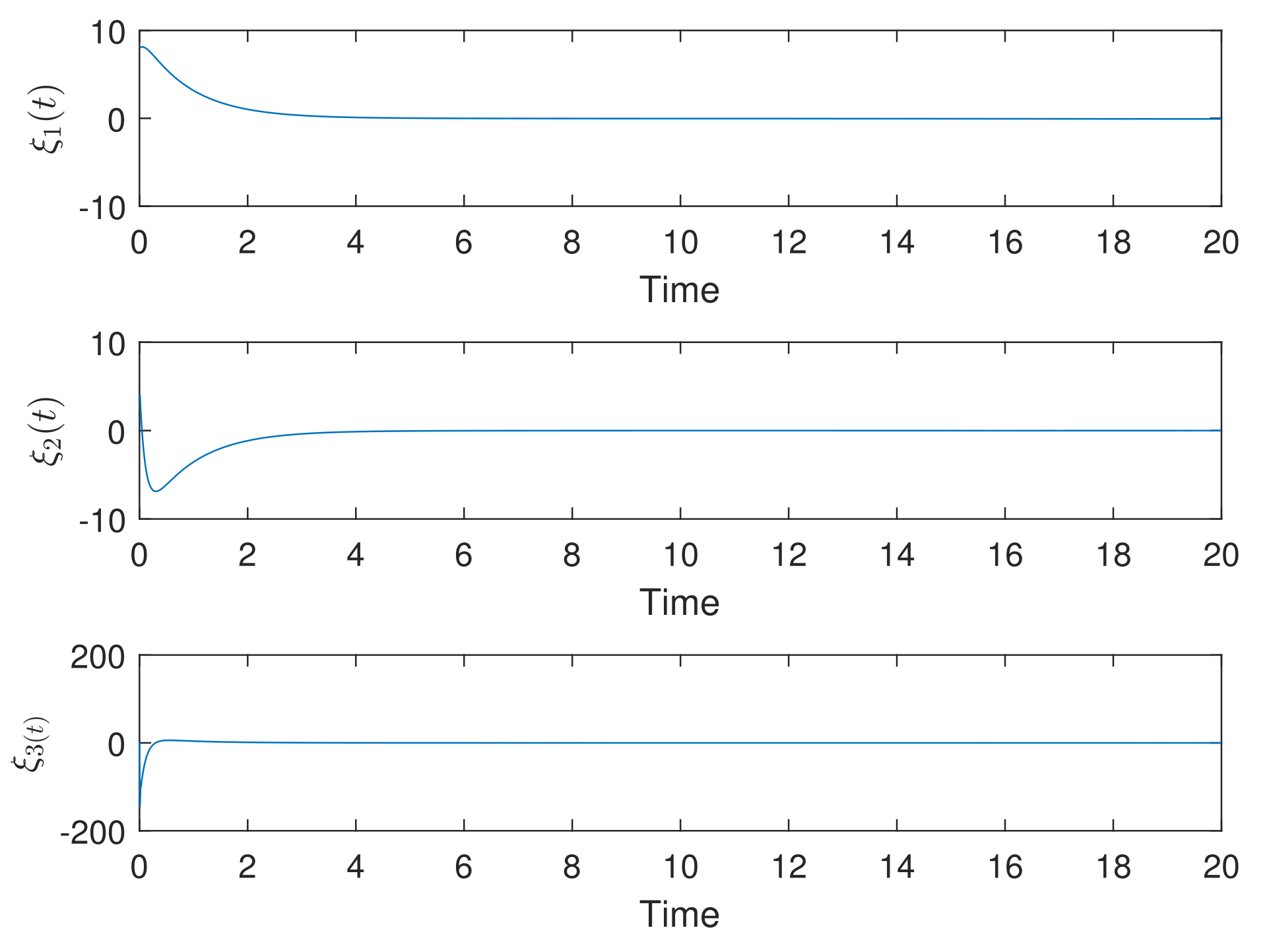
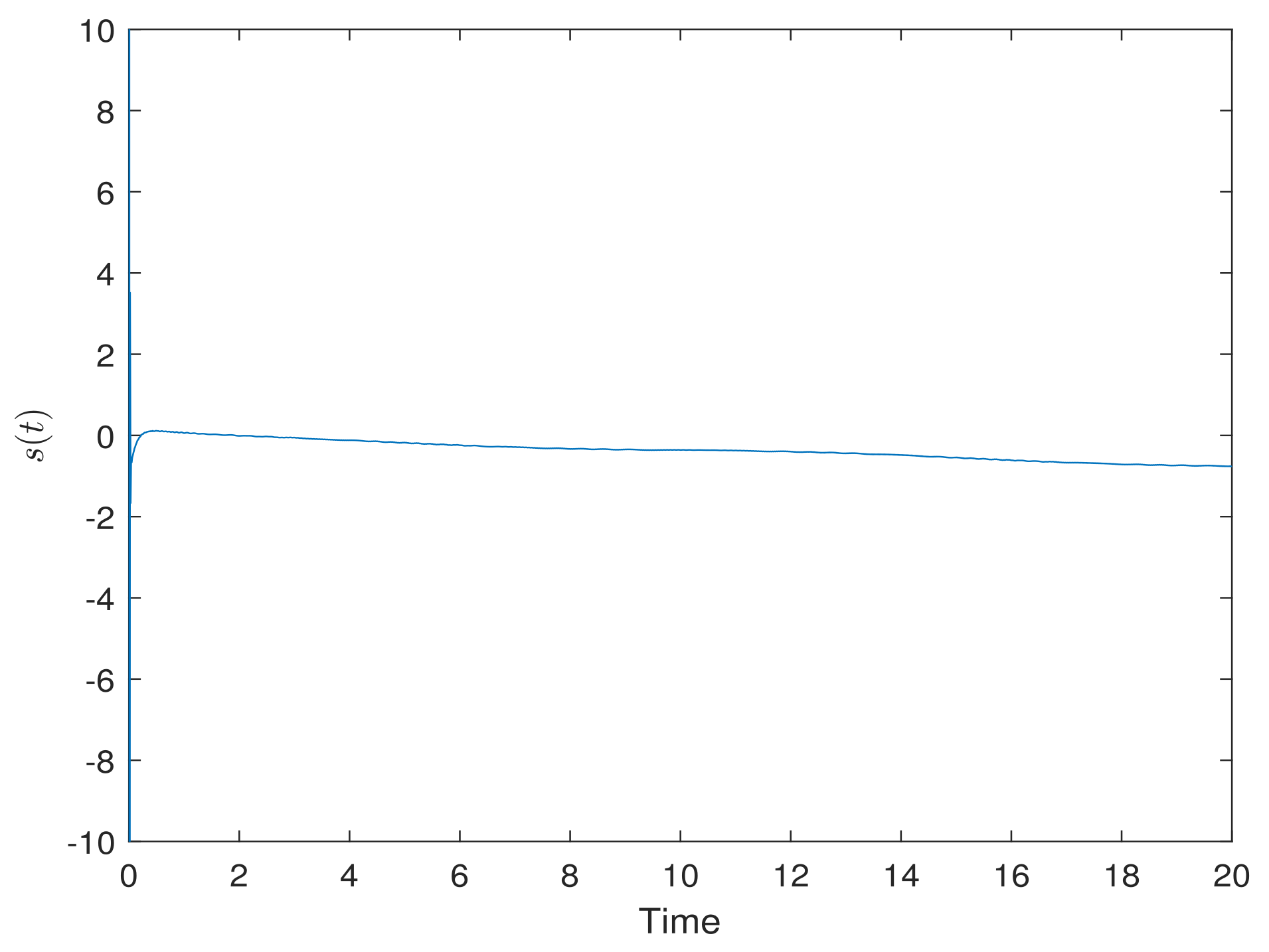
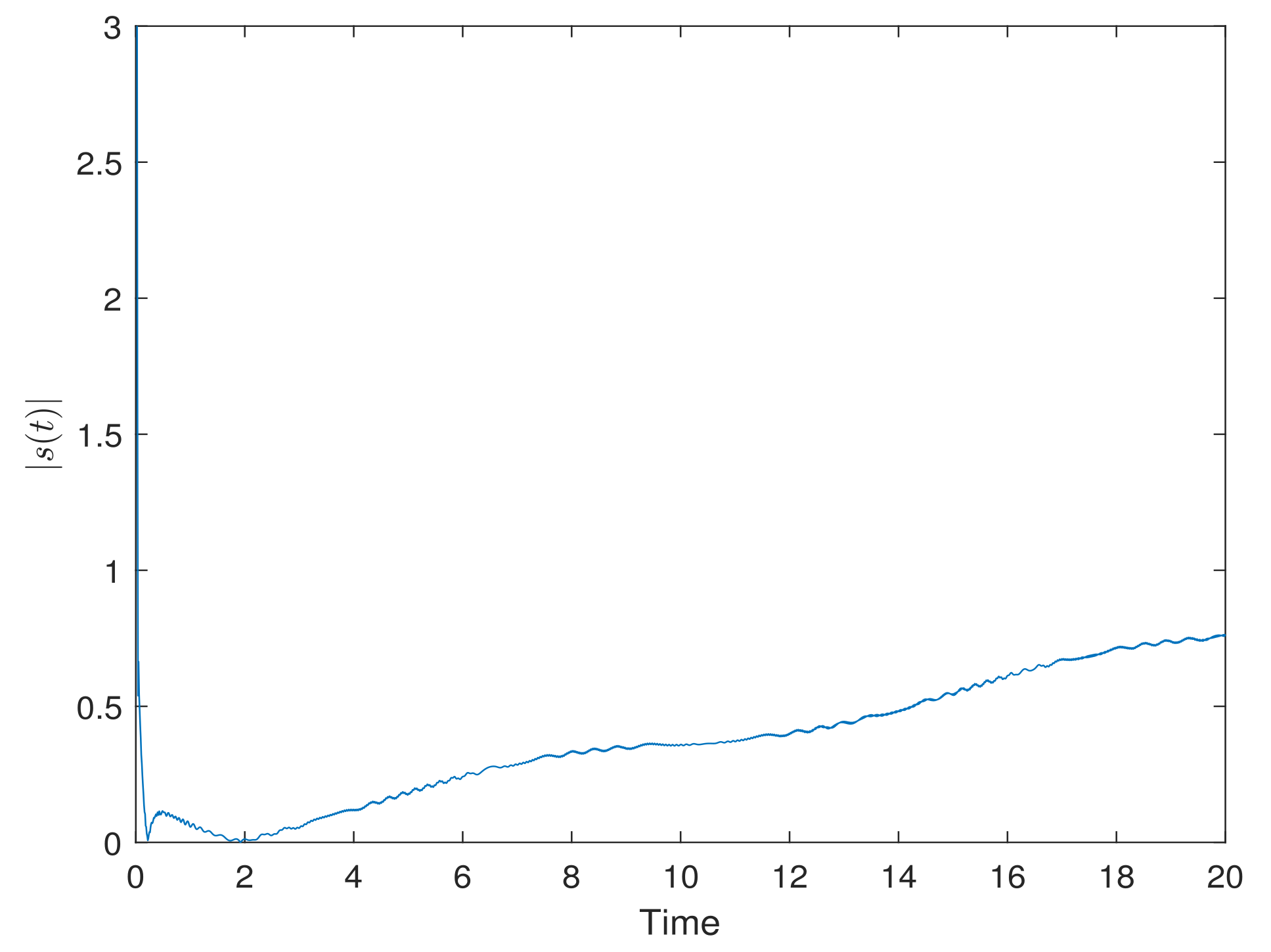
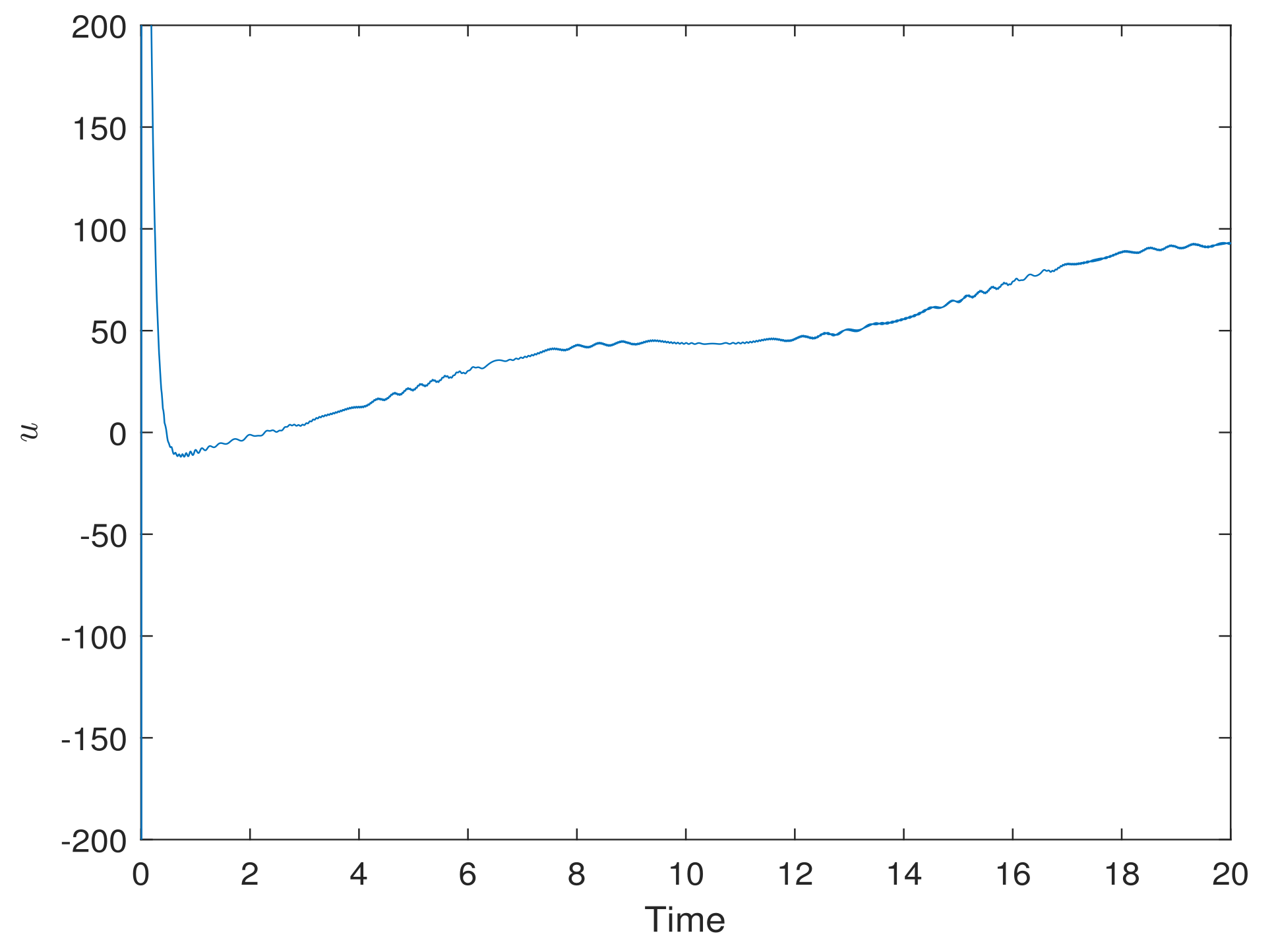
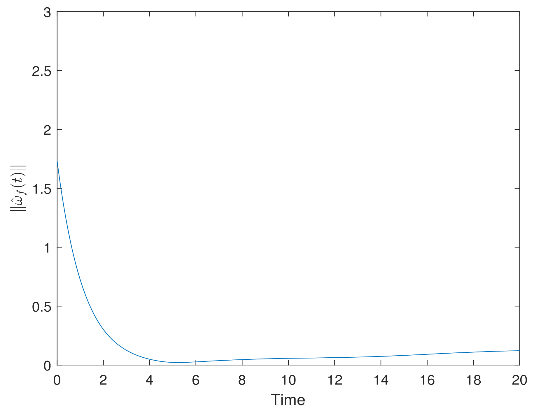
5. Simulation Results

The third-order nonlinear simulation system is introduced as

$$\begin{array}{cc}\hfill {\dot{\chi }}_1\left(t\right)=& {\chi }_2\left(t\right),\hfill \\ \hfill {\dot{\chi }}_2\left(t\right)=& {\chi }_3\left(t\right),\hfill \\ \hfill {\dot{\chi }}_3\left(t\right)=& {\chi }_1\left(t\right)+0.5si{n}^2\left({\chi }_1\left(t\right){\chi }_2\left(t\right)\right)+1.5co{s}^2\left({\chi }_2\left(t\right){\chi }_3\left(t\right)\right)+u,\hfill \end{array}$$

(29)

where the initial values are set as ${\chi }_1\left(0\right)$ = 8, ${\chi }_2\left(0\right)$ = 4, ${\chi }_3\left(0\right)$ = 2. The desired tracking trajectory is described as

$$\begin{array}{cc}\hfill {\dot{\chi }}_{d1}\left(t\right)=& {\chi }_{d2}\left(t\right),\hfill \\ \hfill {\dot{\chi }}_{d2}\left(t\right)=& {\chi }_{d3}\left(t\right),\hfill \\ \hfill {\dot{\chi }}_{d3}\left(t\right)=& -1.6cos\left(0.6t\right),\hfill \end{array}$$

(30)

Corresponding to the sliding term (3), these coefficients are chosen as $c_1=10$, $c_2=10$, and thus the sliding surface is obtained as $s\left(t\right)=10{\xi }_1+10{\xi }_2+{\xi }_3$. The NN corresponding to (11) is set to have 12 neurons, and the centers ${\mu }_i$ are also evenly spaced from $-6$ to 6.

Corresponding to the adaptive law (14) and the adaptive controller (15), the design parameters are set as $k_p=120$, ${\eta }_{sw}=4$, ${\kappa }_f=0.15$ and ${\sigma }_f=5.8$, and the initial values of the NN weight are ${\widehat{\omega }}_f\left(0\right)={\left[0.5\right]}_{12\times 1}$, and the thickness of sliding surface is selected as $\Phi =1.5$.

Figure 1, Figure 2, Figure 3, Figure 4, Figure 5 and Figure 6 show the simulation results of applying the proposed adaptive SMC law (15) with the adaptive law (14). Figure 1 displays the tracking performance in the three state variables ${\chi }_1\left(t\right)$, ${\chi }_2\left(t\right)$, ${\chi }_3\left(t\right)$. Figure 2 shows the tracking errors corresponding to the three variables, and they decrease to zero with time. Figure 3 shows the boundedness of the NN weights. Figure 4 shows the convergence of the sliding variables. These simulation figures further demonstrate that the proposed sliding mode control law can achieve the desired control tasks and objectives.

Figure 5 and Figure 6 show the sliding mode variable and controller of the proposed method. Figure 7 and Figure 8 show the two variables of applying the traditional sliding method that does not consider the boundary layer method. In comparison, the proposed method can significantly alleviated the chattering phenomenon; therefore, it can be concluded that the sliding controller can have better stability than the traditional method.

6. Conclusions

In this article, in order to obtain a better tracking performance with system robustness and to eliminate the undesired chattering phenomenon in the control input signal, we propose an adaptive NN sliding mode control algorithm for a class of unknown dynamic high-order SISO nonlinear systems. Since the system dynamic is assumed to be unknown, we introduce NN to compensate those unknown functions. Furthermore, we replace the discontinuous switching control with a continuous proportional function. In this way, the chattering in control input will be suppressed well. According to the Lyapunov stability theorem, we can verify the effectiveness of the control law. Finally, the simulation results also show that our controller can achieve the desired tracking performance.

References

1. Hauser, J.; Sastry, S.; Meyer, G. Nonlinear control design for slightly non-minimum phase systems: Application to V/STOL aircraft. Automatica 1992, 28, 665–679. [Google Scholar] [CrossRef]
2. Soares, O.; Gonçalves, H.; Martins, A.; Carvalho, A. Nonlinear control of the doubly-fed induction generator in wind power systems. Renew. Energy 2010, 35, 1662–1670. [Google Scholar] [CrossRef]
3. Sirouspour, M.; Salcudean, S. Nonlinear control of hydraulic robots. IEEE Trans. Robot. Autom. 2001, 17, 173–182. [Google Scholar] [CrossRef] [Green Version]
4. Polyakov, A. Sliding mode control design using canonical homogeneous norm. Int. J. Robust Nonlinear Control 2019, 29, 682–701. [Google Scholar] [CrossRef] [Green Version]
5. Difonzo, F.V. Isochronous Attainable Manifolds for Piecewise Smooth Dynamical Systems. Qual. Theory Dyn. Syst. 2022, 21, 6. [Google Scholar] [CrossRef]
6. Kaklamanos, P.; Kristiansen, K.U. Regularization and Geometry of Piecewise Smooth Systems with Intersecting Discontinuity Sets. SIAM J. Appl. Dyn. Syst. 2019, 18, 1225–1264. [Google Scholar] [CrossRef]
7. Utkin, V.I.; Poznyak, A.S. Adaptive sliding mode control with application to super-twist algorithm: Equivalent control method. Automatica 2013, 49, 39–47. [Google Scholar] [CrossRef]
8. Han, Y.; Liu, X. Continuous higher-order sliding mode control with time-varying gain for a class of uncertain nonlinear systems. ISA Trans. 2016, 62, 193–201. [Google Scholar] [CrossRef]
9. SIRA-RAMÍREZ, H. On the dynamical sliding mode control of nonlinear systems. Int. J. Control 1993, 57, 1039–1061. [Google Scholar] [CrossRef]
10. Polyakov, A.; Fridman, L. Stability notions and Lyapunov functions for sliding mode control systems. J. Frankl. Inst. 2014, 351, 1831–1865. [Google Scholar] [CrossRef] [Green Version]
11. Precup, R.E.; Radac, M.B.; Roman, R.C.; Petriu, E.M. Model-free sliding mode control of nonlinear systems: Algorithms and experiments. Inf. Sci. 2017, 381, 176–192. [Google Scholar] [CrossRef]
12. Yang, X.; Lu, J. Finite-Time Synchronization of Coupled Networks with Markovian Topology and Impulsive Effects. IEEE Trans. Autom. Control 2016, 61, 2256–2261. [Google Scholar] [CrossRef]
13. Bartolini, G.; Pisano, A.; Punta, E.; Usai, E. A survey of applications of second-order sliding mode control to mechanical systems. Int. J. Control 2003, 76, 875–892. [Google Scholar] [CrossRef]
14. Islam, S.; Liu, X.P. Robust Sliding Mode Control for Robot Manipulators. IEEE Trans. Ind. Electron. 2011, 58, 2444–2453. [Google Scholar] [CrossRef]
15. Utkin, V. Sliding mode control design principles and applications to electric drives. IEEE Trans. Ind. Electron. 1993, 40, 23–36. [Google Scholar] [CrossRef] [Green Version]
16. Chen, M.; Wu, Q.X.; Cui, R.X. Terminal sliding mode tracking control for a class of SISO uncertain nonlinear systems. ISA Trans. 2013, 52, 198–206. [Google Scholar] [CrossRef]
17. Cao, Y.; Wang, Z.C.; Liu, F.; Li, P.; Xie, G. Bio-Inspired Speed Curve Optimization and Sliding Mode Tracking Control for Subway Trains. IEEE Trans. Veh. Technol. 2019, 68, 6331–6342. [Google Scholar] [CrossRef]
18. Yao, D.; Li, H.; Lu, R.; Shi, Y. Distributed Sliding-Mode Tracking Control of Second-Order Nonlinear Multiagent Systems: An Event-Triggered Approach. IEEE Trans. Cybern. 2020, 50, 3892–3902. [Google Scholar] [CrossRef]
19. Wen, G.; Xu, L.; Li, B. Optimized Backstepping Tracking Control Using Reinforcement Learning for a Class of Stochastic Nonlinear Strict-Feedback Systems. IEEE Trans. Neural Netw. Learn. Syst. 2022. early access. [Google Scholar] [CrossRef]
20. Wen, G.; Li, B.; Niu, B. Optimized Backstepping Control Using Reinforcement Learning of Observer-Critic-Actor Architecture Based on Fuzzy System for a Class of Nonlinear Strict-Feedback Systems. IEEE Trans. Fuzzy Syst. 2022. early access. [Google Scholar] [CrossRef]
21. Fischle, K.; Schroder, D. An improved stable adaptive fuzzy control method. IEEE Trans. Fuzzy Syst. 1999, 7, 27–40. [Google Scholar] [CrossRef]
22. Khonchaiyaphum, I.; Samorn, N.; Botmart, T.; Mukdasai, K. Finite-Time Passivity Analysis of Neutral-Type Neural Networks with Mixed Time-Varying Delays. Mathematics 2021, 9, 3321. [Google Scholar] [CrossRef]
23. Singkibud, K.M.P. Robust passivity analysis of uncertain neutral-type neural networks with distributed interval time-varying delay under the effects of leakage delay. J. Math. Comput. Sci. 2022, 26, 269–290. [Google Scholar] [CrossRef]
24. Tang, R.; Su, H.; Zou, Y.; Yang, X. Finite-Time Synchronization of Markovian Coupled Neural Networks with Delays via Intermittent Quantized Control: Linear Programming Approach. IEEE Trans. Neural Netw. Learn. Syst. 2021. early access. [Google Scholar] [CrossRef]
25. Plestan, F.; Shtessel, Y.; Brégeault, V.; Poznyak, A. New methodologies for adaptive sliding mode control. Int. J. Control 2010, 83, 1907–1919. [Google Scholar] [CrossRef] [Green Version]
26. Huang, Y.J.; Kuo, T.C.; Chang, S.H. Adaptive Sliding-Mode Control for Nonlinear Systems with Uncertain Parameters. IEEE Trans. Syst. Man Cybern. Part B (Cybern.) 2008, 38, 534–539. [Google Scholar] [CrossRef]
27. Tang, R.; Yang, X.; Wan, X. Finite-time cluster synchronization for a class of fuzzy cellular neural networks via non-chattering quantized controllers. Neural Netw. 2019, 113, 79–90. [Google Scholar] [CrossRef]
28. Tang, R.; Yang, X.; Wan, X.; Zou, Y.; Cheng, Z.; Fardoun, H.M. Finite-time synchronization of nonidentical BAM discontinuous fuzzy neural networks with delays and impulsive effects via non-chattering quantized control. Commun. Nonlinear Sci. Numer. Simul. 2019, 78, 104893. [Google Scholar] [CrossRef]
29. Utkin, V.; Lee, H. Chattering problem in sliding mode control systems. IFAC Proc. Vol. 2006, 39, 1. [Google Scholar] [CrossRef]
30. Bartolini, G.; Ferrara, A.; Utkin, V. Adaptive sliding mode control in discrete-time systems. Automatica 1995, 31, 769–773. [Google Scholar] [CrossRef]
31. Yang, X.; Lam, J.; Ho, D.W.C.; Feng, Z. Fixed-Time Synchronization of Complex Networks with Impulsive Effects via Nonchattering Control. IEEE Trans. Autom. Control 2017, 62, 5511–5521. [Google Scholar] [CrossRef]
32. Parra-Vega, V.; Hirzinger, G. Chattering-free sliding mode control for a class of nonlinear mechanical systems. Int. J. Robust Nonlinear Control 2001, 11, 1161–1178. [Google Scholar] [CrossRef]
33. Feng, Y.; Yu, X.; Han, F. On nonsingular terminal sliding-mode control of nonlinear systems. Automatica 2013, 49, 1715–1722. [Google Scholar] [CrossRef]
34. Guo, Y.; Huang, B.; Li, A.J.; Wang, C.Q. Integral sliding mode control for Euler–Lagrange systems with input saturation. Int. J. Robust Nonlinear Control 2019, 29, 1088–1100. [Google Scholar] [CrossRef]
35. Feng, Y.; Han, F.; Yu, X. Chattering free full-order sliding-mode control. Automatica 2014, 50, 1310–1314. [Google Scholar] [CrossRef]
36. Sun, Z.; Zhang, G.; Yi, B.; Zhang, W. Practical proportional integral sliding mode control for underactuated surface ships in the fields of marine practice. Ocean Eng. 2017, 142, 217–223. [Google Scholar] [CrossRef]
37. Mobayen, S. An adaptive chattering-free PID sliding mode control based on dynamic sliding manifolds for a class of uncertain nonlinear systems. Nonlinear Dyn. 2015, 82, 53–60. [Google Scholar] [CrossRef]
38. Boiko, I.M. Chattering in sliding mode control systems with boundary layer approximation of discontinuous control. Int. J. Syst. Sci. 2013, 44, 1126–1133. [Google Scholar] [CrossRef]
39. Kuo, T.C.; Huang, Y.J.; Chang, S.H. Sliding mode control with self-tuning law for uncertain nonlinear systems. ISA Trans. 2008, 47, 171–178. [Google Scholar] [CrossRef]
40. Wen, G.; Chen, C.L.P.; Ge, S.S. Simplified Optimized Backstepping Control for a Class of Nonlinear Strict-Feedback Systems with Unknown Dynamic Functions. IEEE Trans. Cybern. 2021, 51, 4567–4580. [Google Scholar] [CrossRef]
41. Li, S.; An, X.; Ding, L.; Wang, Q.; Gao, H.; Hou, Y.; Deng, Z. Adaptive Neural Network-Based Finite-Time Tracking Control for Nonstrict Nonaffined MIMO Nonlinear Systems. IEEE Trans. Syst. Man Cybern. Syst. 2021, 51, 4814–4824. [Google Scholar] [CrossRef]
42. Zhu, J.; Wen, G.; Li, B. Decentralized adaptive formation control based on sliding mode strategy for a class of second-order nonlinear unknown dynamic multi-agent systems. Int. J. Adapt. Control. Signal Process. 2022, 36, 1045–1058. [Google Scholar] [CrossRef]
43. Wen, G.; Chen, C.L.P.; Li, B. Optimized Formation Control Using Simplified Reinforcement Learning for a Class of Multiagent Systems with Unknown Dynamics. IEEE Trans. Ind. Electron. 2020, 67, 7879–7888. [Google Scholar] [CrossRef]
Figure 1. The tracking performance of three state variables χ 1 , χ 2 and χ 3 .
Mathematics 10 01182 g001
Figure 2. The convergence of three tracking errors ξ 1 , ξ 2 and ξ 3 .
Mathematics 10 01182 g002
Figure 3. The boundedness of the adaptive NN weight ω ^ f .
Mathematics 10 01182 g003
Figure 4. The convergence of sliding variable s ( t ) .
Mathematics 10 01182 g004
Figure 5. The sliding variable | s ( t ) | of implementing the proposed method.
Mathematics 10 01182 g005
Figure 6. The controller u of the proposed method.
Mathematics 10 01182 g006
Figure 7. The chattering phenomenon is arisen in the sliding variable | s ( t ) | of implementing the control u without the boundary layer.
Mathematics 10 01182 g007
Figure 8. The chattering phenomenon is arisen in the control u without the boundary layer.
Mathematics 10 01182 g008
Publisher’s Note: MDPI stays neutral with regard to jurisdictional claims in published maps and institutional affiliations.