A Numerical Method for Multispecies Populations in a Moving Domain Using Combined Masses

Abstract

This paper concerns the numerical evolution of two interacting species satisfying coupled reaction–diffusion equations in one dimension which inhabit the same part of a moving domain. The domain has both moving external boundaries and moving interior interfaces where species may arise, overlap, or disappear. Numerically, a moving finite volume method is used in which node movement is generated by local mass preservation, which includes a general combined mass strategy for species occupying overlapping domains. The method is illustrated by a test case in which a range of parameters is explored.

1. Introduction

Many simulation problems over a vast range of different sectors including physics, finance, biology, and many more, can be described by partial differential equation models that exhibit a priori unknown sets such as interfaces, moving boundaries, shocks, etc.

Moving or free boundary problems have emerged in increasing number in recent years, especially in ecology, for modelling species interactions and generally for gaining insights into population dynamics. Many theoretical results for general models in ecology including competition–diffusion models are found in [1,2,3,4,5,6] and references cited therein. While the theoretical analysis of free boundary problems in ecology is well represented in the literature, there are fewer studies on the implementation of numerical methods for solving such problems, partly due to the presence of moving boundaries.

The approximate solution of free and moving boundary problems is challenging since a higher resolution is usually required in the vicinity of boundaries where a change in the slope of the solution is located, often occupying a central position within the domain.

In reference [7], the authors have used both front tracking and front fixing approaches to numerically solve competition–diffusion models with two free boundaries. The approach involves the use of a fixed grid to locate the position of the moving boundaries, which are then tracked explicitly. However, for solutions possessing sharp spatial transitions that move, such as free or moving boundaries, a fixed mesh method is generally considered inefficient since the very small spatial step required for resolution of the boundary leads to an extremely small time step due to the stiffness of the system.

Over the years, adaptive grid methods have been used successfully to solve free and moving boundary problems. Such methods automatically adjust the size of the space step to better approximate critical regions of high spatial activity without the use of a large number of nodes. The techniques of adaptive grid methods include the addition or removal of nodes in the domain at discrete time levels and the dynamic movement of existing nodes continuously in time to track the features of interest. The latter, also known as moving mesh methods, becomes preferable if the nodes move smoothly along with the solution evolution, while the former includes the constant addition or removal of nodes followed by a solution interpolation between the nodes.

The conservation method is a moving mesh method in which an integral is used to preserve a desired conserved quantity, e.g., mass, within each patch of elements, from which node velocities are constructed. A moving mesh equation is extracted and solved in association with the PDE(s).

A similar approach was used in [8] where the method was applied to several one-dimensional moving boundary problems, including the mass-conserving porous medium equation, Richards’ equation in hydrology, and the Crank–Gupta problem that does not conserve mass. Finite element versions of the velocity-based moving mesh approach has been used by Baines, Hubbard and Jimack in [9,10] and by Baines, Hubbard, Jimack and Mahmood in [11]. More recently, the approach of [8] was used in [12] for solving the competition–diffusion system of [13], in which species are spatially segregated due to high competition and interact only through a moving interface. The results in [12] gave confidence that the method is numerically stable and robust for a wide choice of parameter values.

Even though moving mesh methods have proved to be efficient and reliable, they can be challenging when the system being solved includes coupled PDEs and the solution variables occupy distinct but overlapping domains.

The novelty of this paper lies in the theoretical and numerical treatment of moving boundaries in population dynamics, as well as a combined approach for cohabiting species, which are not standard in the numerical modelling literature. The emphasis of the paper is on the role of the moving mesh method based on conservation in tracking free and moving boundaries in population dynamics.

Motivated by the work in [12], we apply the moving mesh finite volume method based on conservation for the general case of the competition–diffusion system of [13], where coupled species can coexist in space but still compete for common resources.

1.1. The Competition–Diffusion System of Cohabiting Species with Moving Boundaries

In order to demonstrate the features of the numerical method we have chosen the one-dimensional classical Lotka–Volterra system

$$\frac{\partial u}{\partial t}={\delta }_1\frac{{\partial }^{2}u}{\partial x^2}+f(u,v)ux\in {\mathcal{R}}_1\left(t\right),t>0$$

(1)

$$\frac{\partial v}{\partial t}={\delta }_2\frac{{\partial }^{2}v}{\partial x^2}+g(u,v)vx\in {\mathcal{R}}_2\left(t\right)t>0$$

(2)

where $f(u,v)=r_1\left(1-\frac{u+K_{1}v}{k_1}\right)$ and $g(u,v)=r_2\left(1-\frac{v+K_{2}u}{k_2}\right)$. Here u and v are the densities of two competing species that move by diffusion in space, ${\delta }_p$ is the diffusion rate, $r_p$ is the intrinsic growth rate, $K_p$ is the carrying capacity, and $k_p$ is the competition rate ($p=1,2$). All the parameters are positive constants. The domains $\mathcal{R}$${}_1\left(t\right)$ and $\mathcal{R}$${}_2\left(t\right)$ are occupied by species u and v, respectively, and partly overlap (see Figure 1).

1.1.1. Boundary Conditions

A zero Neumann boundary condition is imposed, i.e.,

$$\frac{\partial u}{\partial x}=0t>0,x=0.$$

on u at the fixed left-hand boundary ($x=0$) of the whole domain $\mathcal{R}$${}_1\left(t\right)$∪$\mathcal{R}$${}_2\left(t\right)$, (see Figure 1), which implies that there is no migration across the left-hand boundary.

1.1.2. Interface Conditions

The dynamics of the two inner moving boundaries $H\left(t\right)$ and $Z\left(t\right)$, from the continuity of net flux, are

$$\frac{\mathrm{d}H}{\mathrm{d}t}=-\frac{{\delta }_1}{K_1}{\left.\left(\frac{\partial u}{\partial x}\right)\right|}_{x=H}$$

(3)

and

$$\frac{\mathrm{d}Z}{\mathrm{d}t}=-\frac{{\delta }_2}{K_2}{\left.\left(\frac{\partial v}{\partial x}\right)\right|}_{x=Z}$$

(4)

We impose $u\left(H\right(t),t)=0$ and $v\left(Z\right(t),t)=0$.

1.1.3. Free Boundary Condition

Lastly, the right-hand side boundary $S\left(t\right)$ of species 2 is taken to be a free boundary, which is assigned the condition

$$\frac{\mathrm{d}S}{\mathrm{d}t}=-\frac{{\delta }_2}{\mu }{\left.\left(\frac{\partial v}{\partial x}\right)\right|}_{x=S}$$

(5)

where $\mu$ is inversely proportional to the preferred population density at the spreading front. For the ecological background of free and moving boundary conditions refer to [14].

The difference between the model in [13] and this one is that here, the species are only partly segregated initially, with a region in the middle of the domain where species coexist, as shown in Figure 1.

By contrast, in [12] the application of the moving mesh method to the two-species problem is straightforward as there is no coupling between the equations. The nonlinear reaction terms in each equation depend only on the local species and not on that of the competitor. Moreover, each species occupies a separate part of the domain.

The aim of this paper is to solve the above system of competitive species using a moving mesh finite volume method based on the conservation of mass and a known net inward flux $q\left(t\right)$ at $x=0$.

The layout of the paper is as follows. In Section 2.1, we recall the basics of the conservation method and state algorithms for solving mass and nonmass conserving problems using the moving mesh finite volume based on mass balance.

In Section 2.2, we introduce a combined mass approach in which the competition–diffusion system (1) and (2) is solved on a single mesh, thus avoiding interpolation to approximate f and g at each time step. The essential difference in the approach is the use of the combined mass in overlapped domains. Following the algorithm of Section 2.1.5 and the use of a combined mass approach of Section 2.2, we provide a detailed solution for approximating the competition system (1) and (2). Section 3 provides illustrations for a variety of parameter combinations. Finally, Section 4 gives a brief discussion of the method, the results, and potential research directions.

2. Materials and Methods

2.1. A Solution Based on the Conservation Method

In what follows, m refers to an interval and j or i refers to a node. We introduce a time-dependent space coordinate $\tilde{x}(x,t)$, abbreviated to $\tilde{x}\left(t\right)$ at a specific x, which coincides instantaneously with the fixed coordinate x in the domain $\left(a\right(t),b(t\left)\right)$. Let $\Delta \tilde{x}$ denote the interval between adjacent moving nodes. We follow an interval $\Delta {\tilde{x}}_m$ possessing a density $u_m(\tilde{x},t)$. The mass in the interval is

$${\theta }_m\left(t\right)=u_m\left(t\right)\Delta {\tilde{x}}_m,$$

(6)

and the total mass in the moving domain $\left(a\right(t),b(t\left)\right)$ is

$$\theta \left(t\right)=\sum _m{u}_m\left(t\right)\Delta {\tilde{x}}_m.$$

By mass balance, the rate of change of the mass ${\theta }_m\left(t\right)$ in the interval m is given by the inward flux $q(\tilde{x},t)$ through the interval boundaries together with the flux due to movement, i.e.,

$${\left[q(\tilde{x},t)\right]}_m+{\left[u(\tilde{x},t)w(\tilde{x},t)\right]}_m,$$

where the notation ${[·]}_m$ denotes the jump in the argument across the interval m.

Since $w(\tilde{x},t)=\Delta \tilde{x}/\Delta t$ to the first order in $\Delta t$, it follows from a mass balance that

$$\frac{\mathrm{d}}{\mathrm{d}t}(u_m\Delta {\tilde{x}}_m)=-{[q(\tilde{x},t)+u(\tilde{x},t)w(\tilde{x},t)]}_m$$

(7)

where $w(\tilde{x},t){|}_m$ denotes a velocity associated with the interval m.

The flux $q(\tilde{x},t)$ is the mass increment within the interval m due to the inward/outward fluxes and the source/sink terms, as provided by the problem.

The overall rate of change of mass in the moving domain $\left(a\right(t),b(t\left)\right)$ is

$$\frac{\mathrm{d}}{\mathrm{d}t}\sum _m{u}_m\Delta {\tilde{x}}_m=-{[q(\tilde{x},t)+u(\tilde{x},t)w(\tilde{x},t)]}_{a\left(t\right)}^{b\left(t\right)}$$

where $q(\tilde{x},t)={\int }_{a\left(t\right)}^{b\left(t\right)}\frac{\partial u}{\partial t}\mathrm{d}x$ and ${\left[u(\tilde{x},t)w(\tilde{x},t)\right]}_{a\left(t\right)}^{b\left(t\right)}$ is the flux jump across the boundaries of the moving domain.

2.1.1. A Method Based on Preservation of Relative Masses

The conservation of mass fractions (CMF) method for those problems that conserve the total mass of the solution, i.e., for which $\theta \left(t\right)$ remains constant for all $t\ge t^0$, is based on the preservation of partial masses by supposing that $\tilde{x}$ moves in such a way that the mass in any interval is independent of time, i.e.,

$$u_m\left(t\right)\Delta {\tilde{x}}_m\left(t\right)=c_m$$

(8)

is constant in time.

Then both sides of (7) are zero and the nodal velocities may be constructed from the zero right-hand side. New $\tilde{x}$ positions are determined by integration and new $u(\tilde{x},t+\Delta t)$ by Equation (6).

For more general problems that do not conserve mass such as the one in Section 1.1, the total mass $\theta \left(t\right)$ varies with time. Therefore, it is inconsistent to suppose that the mass (6) in each interval is constant in time. However, the relative density, defined as $u(\tilde{x},t)/\theta \left(t\right)$, has a total relative mass

$${\int }_{a\left(t\right)}^{b\left(t\right)}\frac{u(\tilde{x},t)}{\theta \left(t\right)}\mathrm{d}x$$

which equals unity. It is therefore consistent to suppose that the local relative mass,

$${\int }_m\frac{u(\tilde{x},t)}{\theta \left(t\right)}\mathrm{d}x$$

(9)

in a cell m is conserved in time. The conservation of the relative mass in each subinterval can therefore be used to generate fluxes and velocities to move the nodes. The approach requires the total mass to be given as part of the problem.

The relative CMF method can be described as follows. Define a relative density

$${\widehat{u}}_m=\frac{u_m}{\theta \left(t\right)}$$

(10)

where $\theta \left(t\right)$ is the current total mass. Then, by (9), the relative mass in cell m can be written

$${\int }_m{\widehat{u}}_m(x,t)\mathrm{d}x={\gamma }_m,$$

(11)

constant in time. Summing ${\gamma }_m$ over m gives 1. Furthermore, by conservation of the relative mass (8), the relative flux jump across cell m is

$${[\widehat{q}+\widehat{u}\widehat{w}]}_m=0$$

(12)

where $\widehat{q}$ is a modified flux. Summing (12) over all intervals m, leads to ${[\widehat{q}+\widehat{u}\widehat{w}]}_a^b=0$. If the argument vanishes at one end of the domain, then $\widehat{q}+\widehat{w}\widehat{u}$ is zero at all nodes and

$$\widehat{w}=-\frac{\widehat{q}}{\widehat{u}}$$

is the relative velocity (provided that $\widehat{u}\ne 0$).

The CMF equations for a mass-conserving problem consist of local conservation of mass (Equation (11)) together with the flux balance (Equation (12)). We remark here that Equations (11) and (12) are equivalent to the Lagrangian and Eulerian conservation laws, respectively, which are coincident for small times.

We relate $\widehat{q}$ to the static $\partial u/\partial t$, which is known from the statement of the problem in Section 1.1. Differentiating (11) and using the Leibniz integral rule for the relative mass,

$$\frac{\mathrm{d}}{\mathrm{d}t}{\int }_m\widehat{u}(x,t)\mathrm{d}x=0={\int }_m\frac{\partial \widehat{u}}{\partial t}\mathrm{d}x+{\left[\widehat{u}\widehat{w}\right]}_m$$

By the relative mass balance Equation (12),

$$0={\left[\widehat{q}\right]}_m+{\left[\widehat{u}\widehat{w}\right]}_m$$

(13)

yielding

$${\left[\widehat{q}\right]}_m={\int }_m\frac{\partial \widehat{u}}{\partial t}\mathrm{d}x$$

(14)

Hence, if u, $\theta$ (therefore $\widehat{u}$) are known, [$\widehat{q}$] can be determined from $\frac{\partial u}{\partial t}$. Since by (10),

$$\frac{\partial \widehat{u}}{\partial t}=\frac{\partial }{\partial t}\left(\frac{u}{\theta }\right)=\frac{1}{\theta }\frac{\partial u}{\partial t}-\frac{\dot{\theta }}{{\theta }^2}u$$

where $\dot{\theta }=d\theta /dt$, then from (14)

$${\left[\widehat{q}\right]}_m=\frac{1}{\theta }{\int }_m\frac{\partial u}{\partial t}\mathrm{d}x-\frac{\dot{\theta }}{{\theta }^2}{\int }_{m}u(x,t)\mathrm{d}x$$

and by (11)

$${\left[\widehat{q}\right]}_m=\frac{1}{\theta }\left({\int }_m\frac{\partial u}{\partial t}\mathrm{d}x-\dot{\theta }{\gamma }_m\right)$$

(15)

where $\partial u/\partial t$ is known from the statement of the problem and the time-independent ${\gamma }_m$ are given by (11), leading to

$${\left[\widehat{u}\widehat{w}\right]}_m=-\frac{1}{\theta }\left({\int }_m\frac{\partial u}{\partial t}\mathrm{d}x-{\gamma }_m\dot{\theta }\right)$$

(16)

by Equation (13). If m denotes the interval between two successive nodes, e.g., $(x_i,x_{i+1})$, the left-hand side of (16) can be written ${\left(\widehat{u}\widehat{w}\right)}_{i+1}-{\left(\widehat{u}\widehat{w}\right)}_i$. For a unique solution of $\widehat{u}\widehat{w}$, the flux $\left[\widehat{u}\widehat{w}\right]$ must be imposed at one point which may be thought of as an “anchor” point. A common choice of an anchor point is at the boundary of the region, such as $x_0^n$, where the value $\widehat{u}\widehat{w}$ is known. Summing from a fixed point at node $x_0$ to ${\tilde{x}}_i$ gives

$${\left(uw\right)}_i-{\left(uw\right)}_0=-\left({\int }_m\frac{\partial u}{\partial t}\mathrm{d}x-{\Gamma }_i\dot{\theta }\right).$$

(17)

since ${\left[\widehat{u}\widehat{w}\right]}_m\theta ={\left[uw\right]}_m$, where ${\Gamma }_i={\sum }_{j=0}^i{\gamma }_j$.

The rate of change $\dot{\theta }\left(t\right)$ of the total mass $\theta \left(t\right)$ can be evaluated using the original PDE. By mass balance, the rate of change of the total mass equals the flux $q(\tilde{x},t)$ (inward/outward fluxes and reaction terms) plus the flux due to motion, i.e.,

$$\frac{\mathrm{d}\theta }{\mathrm{d}t}={\int }_{a\left(t\right)}^{b\left(t\right)}\frac{\partial u}{\partial t}\mathrm{d}x+{\left[uw\right]}_{a\left(t\right)}^{b\left(t\right)}$$

(18)

where w in (18) is given by the problem.

Example 1.

As an example related to the Equations (1) and (2), consider u such that

$$\frac{\partial u}{\partial t}=\delta \frac{{\partial }^{2}u}{\partial x^2}+s(x,t)$$

(19)

where δ is the diffusion coefficient and $s(x,t)$ denotes the source terms.

Substituting Equation (19) into Equations (17) and (18), we can calculate the velocity at each node $w_i$ and $\frac{\partial \theta }{\partial t}$ by integration of the diffusion term, together with the boundary conditions, i.e., the equation for $\frac{d\theta }{dt}$ using (18) and (19) is

$$\frac{\mathrm{d}\theta }{\mathrm{d}t}={\int }_{a\left(t\right)}^{b\left(t\right)}\left(\delta \frac{{\partial }^{2}u}{\partial x^2}+s\right)\mathrm{d}x+{\left[uw\right]}_{a\left(t\right)}^{b\left(t\right)}={\int }_{a\left(t\right)}^{b\left(t\right)}s\mathrm{d}x+{\left[\delta \frac{\partial u}{\partial x}+uw\right]}_{a\left(t\right)}^{b\left(t\right)}$$

(20)

and the equation for the velocity $w_i$ of a node $x_i$ is given from (17) and (19) as

$$w_i=\frac{1}{u_i}\left({\Gamma }_i\dot{\theta }-{\int }_m\left(\delta \frac{{\partial }^{2}u}{\partial x^2}+s\right){\mathrm{d}x+uw|}_0\right)=\frac{1}{u_i}\left({\Gamma }_i\dot{\theta }-{\int }_{m}s\mathrm{d}x-\delta {\left[\frac{\partial u}{\partial x}\right]}_m\right)$$

(21)

where the anchor point is taken to be the fixed node $x_0$ (i.e., $w_0=0$), m is the interval $(x_0,x_i)$, and ${\Gamma }_i$ denotes the summation of all the ${\gamma }_j$ from $j=0$ to i. Note that $\dot{\theta }$ is known from (20).

The example ends here.

Once the velocity w has been found it can be integrated to move the nodes

$$\frac{\mathrm{d}\tilde{x}}{\mathrm{d}t}=w,$$

while the new total mass is found by integrating

$$\frac{\mathrm{d}\theta }{\mathrm{d}t}=Q,$$

(22)

where Q is the known rate of increase of mass.

Finally, having the new positions of $\tilde{x}$ and the new $\theta$, we can use Equations (10) and (11) to update $u(\tilde{x},t)$ from

$${\int }_m{u}_m(\tilde{x},t)\mathrm{d}x={\gamma }_m\theta \left(t\right).$$

(23)

A first-order-in-time finite-difference algorithm based on this theory is as follows.

2.1.2. Finite Difference Method

Given a time step $\Delta t>0$ and a fixed number N of spatial nodes, choose discrete times $t^n=n\Delta t,(n=0,1,\dots )$ and discretise the domain at each time using the nodes ${\tilde{x}}_i^n=\tilde{x}(x_i,t^n)$, $i=0,1,\dots ,N,$ for which $a\left(t^n\right)=x_0^n<x_1^n<\dots <x_N^n=b\left(t^n\right)$. Furthermore, define the approximations $u_i^n\approx u(\tilde{x},t^n)$, $w_i^n\approx w(\tilde{x},t^n)$, ${\theta }^n\approx \theta \left(t^n\right)$, and ${\dot{\theta }}^n\approx \dot{\theta }\left(t^n\right)$. Having defined the notation, we proceed to the initial conditions required for the approximate solution.

2.1.3. Time-Stepping

Time-stepping $x_i$

A first-order-in-time explicit time-stepping scheme for ${\tilde{x}}_i^{n+1}$ from (13) is

$${\tilde{x}}_i^{n+1}={\tilde{x}}_i^n+\Delta t{w}_i^n$$

(24)

Another first-order-in-time explicit time-stepping scheme for (22) that preserves the sign of $\Delta {\tilde{x}}_m$ (thus avoiding mesh tangling) for any positive $\Delta t$ is

$$\Delta {\tilde{x}}_m^{n+1}=\Delta {\tilde{x}}_m^{n}exp\left(\Delta t\frac{\Delta w_m^n}{\Delta {\tilde{x}}_m^n}\right),$$

(25)

which is equivalent to (24) to the first order in $\Delta t$.

Time-stepping $\theta \left(t\right)$

In updating the total mass $\theta \left(t\right)$, it is important to ensure that ${\theta }^{n+1}$ will remain positive so that the condition $u>0$ will not be violated. In the same manner as (25), the exponential time-integration scheme may be used to update $\theta$, i.e.,

$${\theta }^{n+1}={\theta }^{n}exp\left(\Delta t\frac{{\dot{\theta }}^n}{{\theta }^n}\right).$$

(26)

ensuring that ${\theta }^{n+1}>0$. More details on the exponential time-stepping scheme for updating $\tilde{x}$ can be found in [15].

2.1.4. Initial Conditions

Choose initial node positions ${\tilde{x}}_i^0,(i=0,1,\dots ,N)$ with corresponding initial $u_i^0$.

From the initial conditions, we derive $\Delta x_i^0$ and compute the initial value ${\theta }^0$ of the total mass $\theta$, given by the composite trapezoidal scheme applied to (7),

$${\theta }^0=\frac{1}{2}\sum _{i=0}^{N-1}\left({\tilde{x}}_{i+1}^0-{\tilde{x}}_i^0\right)(u_i^0+u_{i+1}^0),$$

(27)

Given ${\theta }^0$, we can compute the approximate relative masses ${\gamma }_m$ of (11) by a first-order-in-space shift to the end of the interval, i.e.,

$${\gamma }_m=\frac{1}{{\theta }^0}({\tilde{x}}_i^0-{\tilde{x}}_{i-1}^0)u_i^0(i=m=1,\dots .,N)$$

(28)

Then, at time $t^n$ for $n=1,2,\dots ,$ given ${\theta }^n$, ${\tilde{x}}_i^n$, and $u_i^n$, we calculate ${\theta }^{n+1}$, ${\tilde{x}}_i^{n+1}$, and $u_i^{n+1}$ as follows:

2.1.5. Algorithm

At each time step n,

• Evaluate the rate of change of the total mass ${\dot{\theta }}^n$ by discretising (18) as the boundary influx, source terms, and flux due to motion as

  $${\left(\frac{\mathrm{d}\theta }{\mathrm{d}t}\right)}^n={\int }_{{\tilde{x}}_0^n}^{{\tilde{x}}_N^n}\frac{\partial u(x,t^n)}{\partial t}\mathrm{d}x+w_{{\tilde{x}}_N}^n{\tilde{u}}_{{\tilde{x}}_N}^n-w_{{\tilde{x}}_0}^n{u}_{{\tilde{x}}_0}^n.$$
• Evaluate the discrete velocity at interior points from (17), specifying an anchor point, say $x_0$, so that the equations for the velocity is given by

  $$w_i^n=\frac{u_0^n{w}_0^n-{\int }_{x_0^n}^{x_i^n}\frac{\partial u(s,t^n)}{\partial t}\mathrm{d}x+{\Gamma }_i\dot{\theta }}{u_i^n},i=1,\dots ,N$$

  (29)

  where ${\Gamma }_i={\sum }_{j=0}^i{\gamma }_j$.
  At the boundaries extrapolate the velocity from interior values. Derive $\Delta w_m^n$ for all intervals.
• Update the new $\Delta {\tilde{x}}_m^{n+1}$ using the exponential time-stepping scheme (25).
• Update ${\theta }^{n+1}$ by the exponential time-stepping scheme (26).
• Recover the solution $u_m^{n+1}$ at the interior points from (23) in the form

  $$u_m^{n+1}=\frac{{\gamma }_m{\theta }^{n+1}}{\Delta {\tilde{x}}_m^{n+1}}m=2,\dots ,N.$$

  (30)

  and determine $u_i^{n+1}$ ($i=2,\dots ,N-1$) by a one-sided approximation, with $u_0^{n+1}$ and $u_N^{n+1}$ being updated either from given boundary conditions or by extrapolation, depending on the nature of the problem.

2.2. Numerical Solution for a Competition–Diffusion System with Two Interfaces and a Moving Boundary

We divide the domain into three regions separated by the two interfaces ($Z\left(t\right)$ and $H\left(t\right)$). Denote by ${\mathcal{R}}_L$ the region on the left-hand-side of the moving boundary $Z\left(t\right)$, and by ${\mathcal{R}}_R$ the region on the right-hand-side of the moving boundary $H\left(t\right)$. The region in the middle, bounded by both moving boundaries $Z\left(t\right)$ and $H\left(t\right)$, is denoted by ${\mathcal{R}}_M$. Note that $v\left(t\right)=0$ in ${\mathcal{R}}_L$$\left(t\right)$ and $u\left(t\right)=0$ in ${\mathcal{R}}_R$$\left(t\right)$.

As discussed above, we are considering the mass at a specific location to be the combined mass of the densities u and v. In the conservation methods the nodal velocities are constructed by supposing that fractions of the corresponding relative mass are held constant in time.

For ease of exposition, we drop the tilde ($\tilde{}$) for the rest of the paper.

At time level $t=t^n$, define time-dependent mesh points

$$0=x_0<x_1^n<\dots <x_{\zeta }^n<\dots <x_{\eta }^n<\dots <x_{N+1}^n=x_{\sigma }^n$$

where $x_{\zeta }^n$ is the node at the moving interface $Z\left(t\right)$ and $x_{\eta }^n$ is the node at the moving interface $H\left(t\right)$. Let $u_i^n$ and $v_i^n$ ($0\le i\le N+1$), approximate $u(x,t)$ and $v(x,t)$ by $u_i^n$ and $v_i^n$, respectively, at these points.

For the initial conditions (at $n=0$) we take the $x_i^0$ to be equally spaced and the $u_i^0$ and $v_i^0$ pointwise from an initial function

$$\begin{array}{ccc}\hfill u(x,0)& =30,\hfill & \hfill (0\le x\le 0.46)\\ \hfill u(x,0)& =480(x-0.2)(0.7-x),\hfill & \hfill (0.46\le x\le 0.7)\\ \hfill u(x,0)& =0,\hfill & \hfill (0.7\le x\le 1)\\ \hfill v(x,0)& =0,\hfill & \hfill (0\le x\le 0.3)\\ \hfill v(x,0)& =480(x-1)(0.3-x),\hfill & \hfill (0.3\le x\le 1)\end{array}$$

as shown in Figure 1.

The initial values ${\theta }_L^0$, ${\theta }_M^0$, and ${\theta }_R^0$ of the total masses $\theta$ in the intervals ${\mathcal{R}}_L,{\mathcal{R}}_M,$ and ${\mathcal{R}}_R$, respectively, are approximated by ${\theta }_L^n\approx {\theta }_L\left(t^n\right)$, ${\theta }_M^n\approx {\theta }_M\left(t^n\right)$, and ${\theta }_R^n\approx {\theta }_R\left(t^n\right)$ of (27) estimated by the composite trapezium rule. The constant-in-time relative masses ${\gamma }_{L,i}$, ${\gamma }_{M,i}$, and ${\gamma }_{R,i}$ in the interval ($x_{i-1}^n,x_i^n$) are approximated from (28). Then, at each time step, we proceed with the following calculations as indicated by the algorithm in Section 2.1.1.

2.3. Velocities at the Moving Boundaries

In order to evaluate the nodal velocities at the moving interfaces and the outer boundary, we apply a one-sided approximation to the derivative terms of Equations (3)–(5) for $x_{\eta }$, $x_{\zeta }$, and $x_{\sigma }$, respectively,

$$\frac{\mathrm{d}\eta }{\mathrm{d}t}=-\frac{{\delta }_1}{K_1}\left(\frac{u\left(\eta \right)-u\left({\eta }^{-}\right)}{x\left(\eta \right)-x\left({\eta }^{-}\right)}\right),$$

(31)

where ${\eta }^{-}$ is the node immediately to the left of $\eta$.

$$\frac{\mathrm{d}\zeta }{\mathrm{d}t}=-\frac{{\delta }_2}{K_2}\left(\frac{v\left({\zeta }^{+}\right)-v\left(\zeta \right)}{x\left({\zeta }^{+}\right)-x\left(\zeta \right)}\right),$$

(32)

where ${\zeta }^{+}$ is the node immediately to the right of $\zeta$.

$$\frac{\mathrm{d}\sigma }{\mathrm{d}t}=-\frac{{\delta }_2}{\mu }\left(\frac{v\left(\sigma \right)-v\left({\sigma }^{-}\right)}{x\left(\sigma \right)-x_{(}{\sigma }^{-})}\right).$$

(33)

where ${\sigma }^{-}$ is the node immediately to the left of $\sigma$.

2.4. Approximating the Velocities and the Rates of Change of the Total Populations

From (29), by setting the anchor point $x_0$, the velocity $w_i^n$ in region ${\mathcal{R}}_L$ satisfies,

$$w_i^n{u}_i^n=u_0^n{w}_0^n-{\int }_{x_0}^{x_i^n}\frac{\partial u(s,t^n)}{\partial t}\mathrm{d}x+{\Gamma }_{L,i}{\dot{\theta }}_L(x_i\in {\mathcal{R}}_L),$$

where ${\Gamma }_{L,i}={\sum }_{j=0}^i{\gamma }_{L,j}$ for $i=1,\dots \zeta -1$.

By substituting the original PDE (1) and applying the boundary condition $w_0=0$, the equation for the node velocities in region ${\mathcal{R}}_L$ is

$$w_i^n=\frac{1}{u_i^n}\left({\Gamma }_{L,i}{\dot{\theta }}_L^n-{\int }_{x_0}^{x_i^n}\left({\delta }_1\frac{{\partial }^{2}u}{\partial x^2}+r_{1}u\left(1-\frac{u}{k_1}\right)\right)\mathrm{d}x\right)$$

(34)

provided that $u_i^n\ne 0$, since $v=0$ in ${\mathcal{R}}_L$.

Applying the integration and the Neumann boundary condition at $x_0$ Equation (34) becomes

$$w_i^n=\frac{1}{u_i^n}\left({\Gamma }_{L,i}{\dot{\theta }}_L^n-{\delta }_1{\left.\frac{\partial u}{\partial x}\right|}_i-{\Phi }_i^n\right),(1\le i\le \zeta -1),$$

(35)

where the derivative term is approximated by a one-sided approximation as ${\Phi }_i$ denotes the reaction terms of Equation (1) approximated by the composite trapezium rule which has summation over $j=0$ and i$\left(i=1,\dots ,\zeta -1\right)$. In order to evaluate $w_i^n$ in (35) we require ${\dot{\theta }}_L^n$.

By setting $x_i=x_{\zeta }$ in (34), due to the boundary conditions and the known velocity at the moving boundary $x_{\zeta }$, we can obtain an equation for ${\dot{\theta }}^n$ in region ${\mathcal{R}}_L$, i.e.,

$${\dot{\theta }}_L^n={\delta }_1\frac{\partial u}{\partial x}{|}_{\zeta }+{\Phi }^n{+uw|}_{\zeta }$$

(36)

since summing ${\gamma }_{L,j}$ over $j=0$ to $\zeta$ gives 1. The summation of the composite trapezoidal rule approximation ${\Phi }^n$ is over $j=0$ and $i=\zeta$.

Similarly, from (29) by taking the anchor point to be $x_{\zeta }$, the velocity $w^n$ in region ${\mathcal{R}}_M$ satisfies

$$w_i^n{u}_i^n=u_{\zeta }^n{w}_{\zeta }^n-{\int }_{x_{\zeta }^n}^{x_i^n}\frac{\partial u(s,t^n)}{\partial t}\mathrm{d}x+{\Gamma }_{M,i}{\dot{\theta }}_M(x_i\in {\mathcal{R}}_M),$$

where ${\Gamma }_{M,i}={\sum }_{j=\zeta }^i{\gamma }_{M,j}$ for $i=\zeta +1,\dots \eta -1$.

By substituting the original PDEs (1) and (2) and applying the boundary conditions, the equation for the node velocities in region ${\mathcal{R}}_M$ is

$$w_i^n=\frac{1}{(u_i^n+v_i^n)}({\Gamma }_{M,i}{\dot{\theta }}_M^n$$

$$-{\int }_{x_{\zeta }^n}^{x_i^n}\left({\delta }_1\frac{{\partial }^{2}u}{\partial x^2}+{\delta }_2\frac{{\partial }^{2}v}{\partial x^2}+r_{1}u\left(1-\frac{u+K_{1}v}{k_1}\right)+r_{2}v\left(1-\frac{v+K_{2}u}{k_2}\right)\right){\mathrm{d}x+(u+v)w|}_{\zeta })$$

(37)

provided that $u_i^n+v_i^n\ne 0$.

Applying the integration, Equation (37) becomes

$$w_i^n=\frac{1}{(u_i^n+v_i^n)}\left({\Gamma }_{M,i}{\dot{\theta }}_M^n-{\delta }_1{\left.\frac{\partial u}{\partial x}\right|}_{\zeta }^i-{\delta }_2{\left.\frac{\partial v}{\partial x}\right|}_{\zeta }^i-{\Psi }_i^n-{{\rm Y}}_i^n{+(u+v)w|}_{\zeta }\right)(\zeta +1\le i\le \eta -1)$$

(38)

where ${\Psi }_i^n$ and ${{\rm Y}}_i^n$ denote the composite trapezoidal rule approximations for the reaction terms of (1) and (2), respectively, with summation from $j=\zeta$ to i$(i=\zeta +1,\dots ,\eta -1)$.

By setting $i=\eta$ and since ${\sum }_{j=\zeta }^{i=\eta }{\gamma }_{M,j}=1$, the equation for ${\dot{\theta }}^n$ in region ${\mathcal{R}}_M$ is given by

$${\dot{\theta }}_M^n={\delta }_1\frac{\partial u}{\partial x}{|}_{\zeta }^{\eta }+{\delta }_2\frac{\partial v}{\partial x}{|}_{\zeta }^{\eta }+{\Psi }^n+{{\rm Y}}^n{+(u+v)w|}_{\zeta }^{\eta }.$$

(39)

Here, the composite trapezoidal rule approximations ${\Psi }^n$ and ${{\rm Y}}^n$ sum from $j=\zeta$ to $i=\eta$.

Finally, from (29) by taking the anchor point $x_{\eta }$, the velocity $w^n$ in region ${\mathcal{R}}_R$ is

$$w_i^n{u}_i^n=u_{\eta }^n{w}_{\eta }^n-{\int }_{x_{\eta }^n}^{x_i^n}\frac{\partial u(s,t^n)}{\partial t}\mathrm{d}x+{\Gamma }_{R,i}{\dot{\theta }}_R(x_i\in {\mathcal{R}}_R),$$

where ${\Gamma }_{R,i}={\sum }_{j=\eta }^i{\gamma }_{R,j}$ for $i=\eta +1,\dots \sigma -1$.

By substituting the original PDE (2), the equation for the node velocities in region ${\mathcal{R}}_R$ is

$$w_i^n=\frac{1}{v_i^n}\left({\Gamma }_{R,i}{\dot{\theta }}_R^n-{\int }_{x_{\eta }^n}^{x_i^n}\left({\delta }_2\frac{{\partial }^{2}v}{\partial x^2}+r_{2}v\left(1-\frac{v}{k_2}\right)\right){\mathrm{d}x+vw|}_{\eta }\right)$$

(40)

since $u=0$ in ${\mathcal{R}}_R$, provided that $v_i^n\ne 0$.

Applying the integration, Equation (40) becomes,

$$w_i^n=\frac{1}{v_i^n}\left({\Gamma }_{R,i}{\dot{\theta }}_R^n-{\delta }_2{\left.\frac{\partial v}{\partial x}\right|}_{\eta }^i-{\Xi }_i^n{+vw|}_{\eta }\right),(\eta +1\le i\le \sigma -1).$$

(41)

${\Xi }_i^n$ is the composite trapezoidal rule approximation of the reaction terms of Equation (2) with summation from $j=\eta$ to i$\left(i=\eta +1,\dots \sigma -1\right)$.

The equation for ${\dot{\theta }}^n$ in region ${\mathcal{R}}_R$ is obtained from Equation (40) by setting $i=\sigma$, i.e.,

$${\dot{\theta }}_R^n={\delta }_2\frac{\partial v}{\partial x}{|}_{\eta }^{\sigma }+{\Xi }^n+vw{{|}_{\sigma }-vw|}_{\eta }$$

(42)

where the composite trapezoidal rule approximation ${\Xi }^n$ sums from $j=\eta$ to $i=\sigma$.

Having found the velocities for all the nodes in the domain, we update the nodal positions.

2.5. Time-Stepping

As discussed in Section 2.1.3, a first-order exponential scheme is used to update both the node positions of $x_i^{n+1}$ and the new ${\theta }^{n+1}$, i.e.,

$$\Delta {\tilde{x}}_i^{n+1}=\Delta {\tilde{x}}_i^{n}exp\left(\Delta t\frac{\Delta w_i^n}{\Delta {\tilde{x}}_i^n}\right)$$

(43)

and

$${\theta }^{n+1}={\theta }^{n}exp\left(\Delta t\frac{{\dot{\theta }}^n}{{\theta }^n}\right).$$

(44)

2.6. Population Densities

Having found the new positions of the nodes, all that is left now is to determine the approximate population densities u and v at the moved nodes at the new time $t=t^{n+1}$.

Once the $x_i^{n+1}$ have been found, we find an approximation solution for the population densities $u^{n+1}$ and $v^{n+1}$. Instead of using the conservation principle as follows by the algorithm in Section 2.1.5, Equation (30), we use the mass balance equations for the u and v local masses to update u and v individually throughout the domain. The rate of change of the mass equals the augmented flux (i.e., inward/outward flux and the flux due to motion) and the reaction terms. Thus, using the velocities and the updated x-positions found above, we can update u and v individually throughout the domain using the Leibniz integral rule or the arbitrary Lagrangian equation [16]:

$$\left(\frac{\mathrm{d}}{\mathrm{d}t}\right){\int }_{x_{i-1}}^{x_i}u\mathrm{d}x={\int }_{x_{i-1}}^{x_i}\frac{\partial u}{\partial t}\mathrm{d}x+{\int }_{x_{i-1}}^{x_i}\frac{\partial }{\partial x}\left(uw\right)\mathrm{d}x(i=0,\dots ,\eta -1)$$

(45)

$$\left(\frac{\mathrm{d}}{\mathrm{d}t}\right){\int }_{x_i}^{x_{i+1}}v\mathrm{d}x={\int }_{x_i}^{x_{i+1}}\frac{\partial v}{\partial t}\mathrm{d}x+{\int }_{x_i}^{x_{i+1}}\frac{\partial }{\partial x}\left(vw\right)\mathrm{d}x(i=\zeta +1,\dots ,N)$$

(46)

Note that $u_i=0$ for $i=\eta ,\dots ,N+1$ and $v_i=0$ for $i=0,\dots ,\zeta$.

In detail, substituting Equations (1) and (2) into the right-hand sides of (45) and (46) gives,

$$={\int }_{x_{i-1}}^{x_i}{\delta }_1\frac{{\partial }^{2}u}{\partial x^2}\mathrm{d}x+{\int }_{x_{i-1}}^{x_i}{r}_{1}u\left(1-\frac{u-K_{1}v}{k_1}\right)\mathrm{d}x+{\int }_{x_{i-1}}^{x_i}\frac{\partial }{\partial x}\left(uw\right)\mathrm{d}x(i=0,\dots ,\eta -1)$$

$$={\int }_{x_i}^{x_{i+1}}{\delta }_2\frac{{\partial }^{2}v}{\partial x^2}\mathrm{d}x+{\int }_{x_i}^{x_{i+1}}{r}_{2}v\left(1-\frac{v-K_{2}u}{k_2}\right)\mathrm{d}x+{\int }_{x_i}^{x_{i+1}}\frac{\partial }{\partial x}\left(vw\right)\mathrm{d}x(i=\zeta +1,\dots ,N)$$

Applying the integration on the right-hand side,

$$={\delta }_1\frac{\partial u}{\partial x}{|}_{i-1}^i+{\int }_{x_{i-1}}^{x_i}{r}_{1}u\left(1-\frac{u-K_{1}v}{k_1}\right){\mathrm{d}x+uw|}_{i-1}^i(i=0,\dots ,\eta -1)$$

$$={\delta }_2\frac{\partial v}{\partial x}{|}_i^{i+1}+{\int }_{x_i}^{x_{i+1}}{r}_{2}v\left(1-\frac{v-K_{2}u}{k_2}\right){\mathrm{d}x+vw|}_i^{i+1}(i=\zeta +1,\dots ,N)$$

Now, integrating in time,

$${\int }_{x_{i-1}}^{x_i}u\mathrm{d}x=\Delta t\left({\delta }_1\frac{\partial u}{\partial x}{|}_{i-1}^i+{\int }_{x_{i-1}}^{x_i}{r}_{1}u\left(1-\frac{u-K_{1}v}{k_1}\right){\mathrm{d}x+uw|}_{i-1}^i\right)(i=0,\dots ,\eta -1)$$

$${\int }_{x_i}^{x_{i+1}}v\mathrm{d}x=\Delta t\left({\delta }_2\frac{\partial v}{\partial x}{|}_i^{i+1}+{\int }_{x_i}^{x_{i+1}}{r}_{2}v\left(1-\frac{v-K_{2}u}{k_2}\right){\mathrm{d}x+vw|}_i^{i+1}\right)(i=\zeta +1,\dots ,N)$$

With ${\varphi }^n=\varphi \left(t^n\right)$ and ${\varphi }_i=\frac{1}{\Delta t}{\int }_{t^n}^{t^{n+1}}\varphi (x_i,t)\mathrm{d}t$,

$$\begin{array}{c}{u}_i^{n+1}=\frac{1}{x_i^{n+1}-x_{i-1}^{n+1}}(u_i^n\left(x_i^n-x_{i-1}^n\right)+\Delta t({\delta }_1\frac{\partial u^n}{\partial x}{|}_{i-1}^i\hfill \\ \hfill +{\int }_{x_{i-1}^n}^{x_i^n}{r}_1{u}^n\left(1-\frac{u^n-K_1{v}^n}{k_1}\right)\mathrm{d}x+u^n{w}^n{|}_{i-1}^i\left)\right)(i=0,\dots ,\eta -1)\end{array}$$

(47)

$$\begin{array}{c}{v}_i^{n+1}=\frac{1}{x_{i+1}^{n+1}-x_i^{n+1}}(v_i^n\left(x_{i+1}^n-x_i^n\right)+\Delta t({\delta }_2\frac{\partial v^n}{\partial x}{|}_i^{i+1}\hfill \\ \hfill -{\int }_{x_i^n}^{x_{i+1}^n}{r}_2{v}^n\left(1-\frac{v^n-K_2{u}^n}{k_2}\right)\mathrm{d}x+v^n{w}^n{|}_i^{i+1}\left)\right)(i=\zeta +1,\dots ,N)\end{array}$$

(48)

The algorithm in this paper for the approximate solution of the Lotka–Volterra competition–diffusion system of cohabiting species (1) and (2) using the moving mesh finite volume method based on conservation and the combined mass procedure can be summarised as follows.

2.7. Algorithm for the Competition–Diffusion System

First, evaluate the combined mass ${\theta }_L$, ${\theta }_M$, and ${\theta }_R$ by (27), noting that $u=0$ in ${\mathcal{R}}_R$ and $v=0$ in ${\mathcal{R}}_L$, and calculate ${\gamma }_m$ in each interval m, for each region by (28).

Then, at each time step, we proceed with the following calculations:

• Evaluate the rate of change of mass in each region ${\dot{\theta }}_L^n$, ${\dot{\theta }}_M^n$, and ${\dot{\theta }}_R^n$ by (36), (39), and (42), respectively.
• Evaluate the velocities at the two interfaces by (31) and (32) and at the free boundary by (33). Calculate the nodal velocities $w_i^{n+1}$ in each region by (35), (38), and (41). For ${\mathcal{R}}_L$, the anchor point is taken at $x_0$, in region ${\mathcal{R}}_M$, it is taken at $x_{\zeta }$, and in region ${\mathcal{R}}_R$ at $x_{\eta }$.
• Update the new nodal positions $x_i^{n+1}$ and the new masses ${\theta }_L^{n+1}$, ${\theta }_M^{n+1}$, and ${\theta }_R^{n+1}$ by the exponential time-stepping scheme ((43) and (44)).
• Recover the solutions $u_i^{n+1}$ for $i=0,\dots ,\eta -1$ and $v_i^{n+1}$ for $i=\zeta +1,\dots ,N$ by the use of the mass balance equations and the updated nodal positions $x_i^{n+1}$ from Equations (47) and (48), respectively.

In order to check whether the procedure of using a single mesh for the combined mass is reliable for solving the two-component Lotka–Volterra competition–diffusion model, we first compared our results against the standard, well-established, moving mesh finite volume method of [8,12], where each species’ equation was solved on a unique mesh and the coupling terms were approximated using interpolation.

3. Results

The model was found to be stable and robust for a variety of parameter choices. Even though the use of the exponential time-stepping scheme ensured that no tangling would occur, it remains an explicit scheme. Therefore, the time step was restricted by stability considerations. For this reason the time step value was set at $\Delta t=0.0005$.

3.1. Parameter Choices

For the following examples, we have used the initial conditions illustrated in Figure 1. The mass of species 2 is set initially to be greater than species 1, and species 2 can escape the overlapping region through the outer right moving boundary. Species 1 is restricted by the left-hand-side stationary boundary where we have imposed a zero Neumann boundary condition which implies no migration. The default variables used for the simulations (${\delta }_1={\delta }_2=0.001$, $K_1=K_2=1$, $k_1=k_2=100$, $r_1=r_2=1$, and $\mu =50$) are similar to the ones used in [12,17] for the extreme case of the competition–diffusion system (1) and (2), presented in [13], where the competition parameters $K_1$ and $K_2$ were very large to spatially segregate the two populations. A sensitivity analysis was carried out by varying one parameter at a time to test the robustness of the results, which showed that the model and the numerical method produced stable results for each parameter change. A selection of results is presented below, which indicates that the method is likely to be able to satisfy the requirements of modelling a wide variety of competition systems.

In the following figures, the initial conditions are shown in black while green, blue, and red indicate, respectively, how the population densities u, $u+v$, and v evolve through time. All results were run with a time step of 0.0005 and we plotted the results for every step of $0.25$.

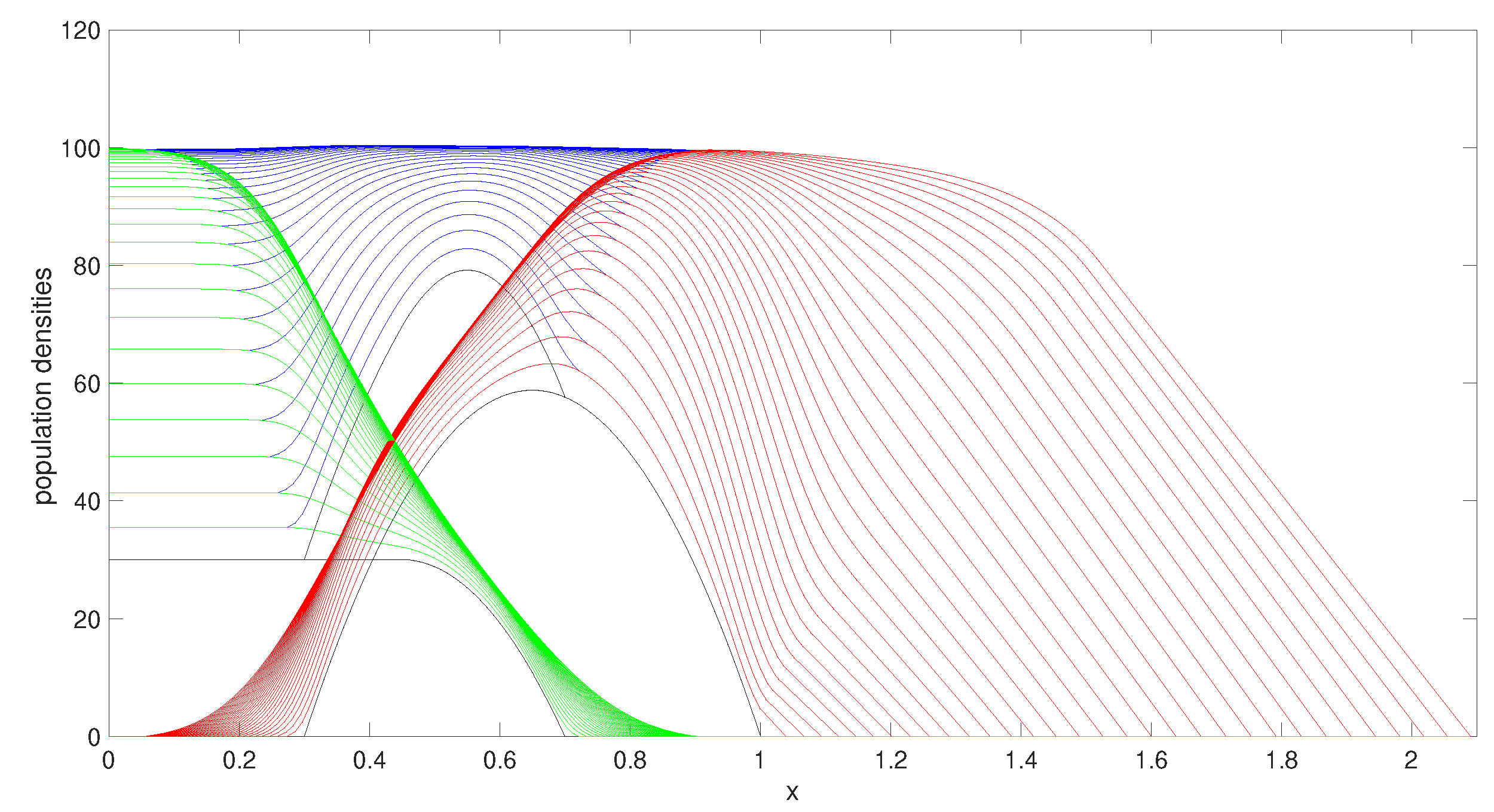
Figure 2 shows the evolution of the populations as time progresses using ${\delta }_1={\delta }_2=0.001$, $K_1=K_2=1$, $k_1=k_2=100$, $r_1=r_2=1$, and $\mu =50$. The two populations have both reached their maximum carrying capacities and individuals are spreading throughout the domain through the moving boundaries.

We investigated other parameter choices. We selected a conservatively representative set of parameters, chosen to demonstrate some of the interesting behaviours that this model is able to describe.

3.1.1. Decreasing the Carrying Capacity $K_2$

For Figure 3, we have used the same parameter values as the example above except for the carrying capacity of species 2, which is set to be lower ($k_2=60$ instead of $k_2=100$). We have restricted the growth of species 2 by lowering its carrying capacity and in comparison to Figure 2, we observe that the decrease in the carrying capacity caused the population to disperse less through the moving boundaries. Species 1 on the other hand has benefited from the restriction of species 2 and increased its mass, and species 1 has dispersed faster in the domain through the moving boundary, taking over most of the domain.

3.1.2. Increasing the Competition Rate $K_2$

The result in Figure 4 is focused on the effect of changing the competition parameter. We have increased the competition parameter of species 2 ($K_2$) by a factor of 5. As shown in Figure 4, due to the high competition of species 2, the population of species 2 is shifting towards the right-hand side of the domain, away from the overlapping region.

3.1.3. Decreasing the Diffusion Coefficient ${\delta }_1$

In Figure 5, we have decreased the diffusion coefficient of species 1 by a factor of 10. As expected, that has restricted the ability of species 1 to disperse in the domain compared to Figure 6.

3.1.4. Decreasing the Parameter $\mu$

Lastly, in Figure 6, we have investigated the $\mu$ parameter in the boundary condition at the right-hand-side outer moving boundary. We set $\mu =1$ instead of 50. In [14], it is shown that $\mu$ is inversely proportional to the preferred population density at the spreading front. Thus, increasing $\frac{1}{\mu }$ causes the population to disperse more through the moving boundary in its effort to increase the population density, as shown in Figure 6. We can also observe that the velocity of the right-hand-side outer moving boundary is increasing at earlier times and remains constant for the rest of the time.

4. Discussion

In this paper, we have described a one-dimensional moving mesh finite volume numerical method based on local mass conservation for the approximate solution of a two-species Lotka–Volterra (L–V) competition system with a free boundary and moving internal interfaces.

The system consists of two species governed by coupled Lotka–Volterra equations in one dimension, partially coexisting in space and competing for common resources. The domain has a moving outer boundary and there are moving interfaces in the interior, where species arise, overlap, or disappear. We therefore considered an L–V model with distinct moving regions in which species are smooth, separated by interfaces with interface conditions.

Numerically, rather than allocate a separate mesh to each species (which would have led to the need for interpolation and a generally messy scheme), we used a single moving mesh for both species and adjusted the solution using the arbitrary Lagrangian Euler (ALE) equations. The mesh is generated by preserving the total sum of local densities (therefore masses) at a point in time. We called this the combined mass approach, which allows a single moving mesh to be used in overlapping regions and handles moving interfaces at points where species arise, overlap, or disappear. The combined mass procedure is general and can be applied to other overlapping situations.

We used a method to move the nodes based on the preservation of relative densities (i.e., those normalised by the total mass), since relative masses are conserved. Once the nodes had been moved, the local densities of each species were computed from the ALE schemes. The procedure generated nodal velocities and nodal displacements, while the densities were recovered using relative conservation. Throughout the paper, we used an exponential time-integrating scheme for nodal intervals, which produces nontangling meshes and is stable for sufficiently small time steps.

We implemented the model for a number of parameter combinations and observed a variety of scenarios. We altered one parameter at a time from the initial set of parameters and observed various effects dominating in turn, as the populations evolve through time. The illustrations indicated that the method was stable for a variety of different set-up parameters and can be applied to many other competition problems.

In certain ecological contexts, reaction–diffusion models may not adequately describe how organisms move and disperse through space. For example, besides the classical Laplacian diffusion in (1) and (2), ecological modellers have included an advection term to describe the ability of living organisms to sense the stimulating signals in the environment and adjust movements accordingly [18]. Many authors have modelled the directed movements of species either through motion along gradients “taxis” or through cross/self-diffusion terms [19,20]. The results of this paper indicate that the methodology can be generalised for more complex equations that are able to more realistically describe the species behaviour and evolution through time.

This paper is proof-of-concept rather than exhaustive and can be refined in a number of ways. Generalisation to two dimensions is a priority and is currently under investigation. Furthermore, the time step can be made semi-implicit, allowing larger time steps, albeit at the risk of losing accuracy.

We conclude that the approach can be used on a variety of ecological models involving multispecies populations and moving boundaries, and is capable of simulating complex behaviour.

Future work will also include the adaptation of the parameters for use on empirical data sets and comparison of results against observations.