
Prophesying the Short-Term Dynamics of the Crude Oil Future Price by Adopting the Survival of the Fittest Principle of Improved Grey Optimization and Extreme Learning Machine


 , ,
, ,  and
and
Abstract
:1. Introduction
- (a).
- (b).
- The hybridizing optimization methods offer their own set of benefits and also need meticulous readjustment of specific parameters of the algorithm. In the ELM network, the global best is regarded as the least objective value (error), whereas, the global worst is considered the greatest objective value (error). To start with, the biases and weights are chosen randomly, and the weight is modified using optimization techniques in the following iteration, and so on until the process is complete.
- (c).
- The IGWO [47] method is utilized to achieve the right balance between exploration and exploitation, as well as to speed up the convergence rate and thereby enhance the accuracy of the ELM network.
- (d).
- In the proposed model of IGWO, where DE speeds up the convergence rate, the SOF principle in IGWO [47] is capable of handling the non-linearity nature of the crude oil price.
- (e).
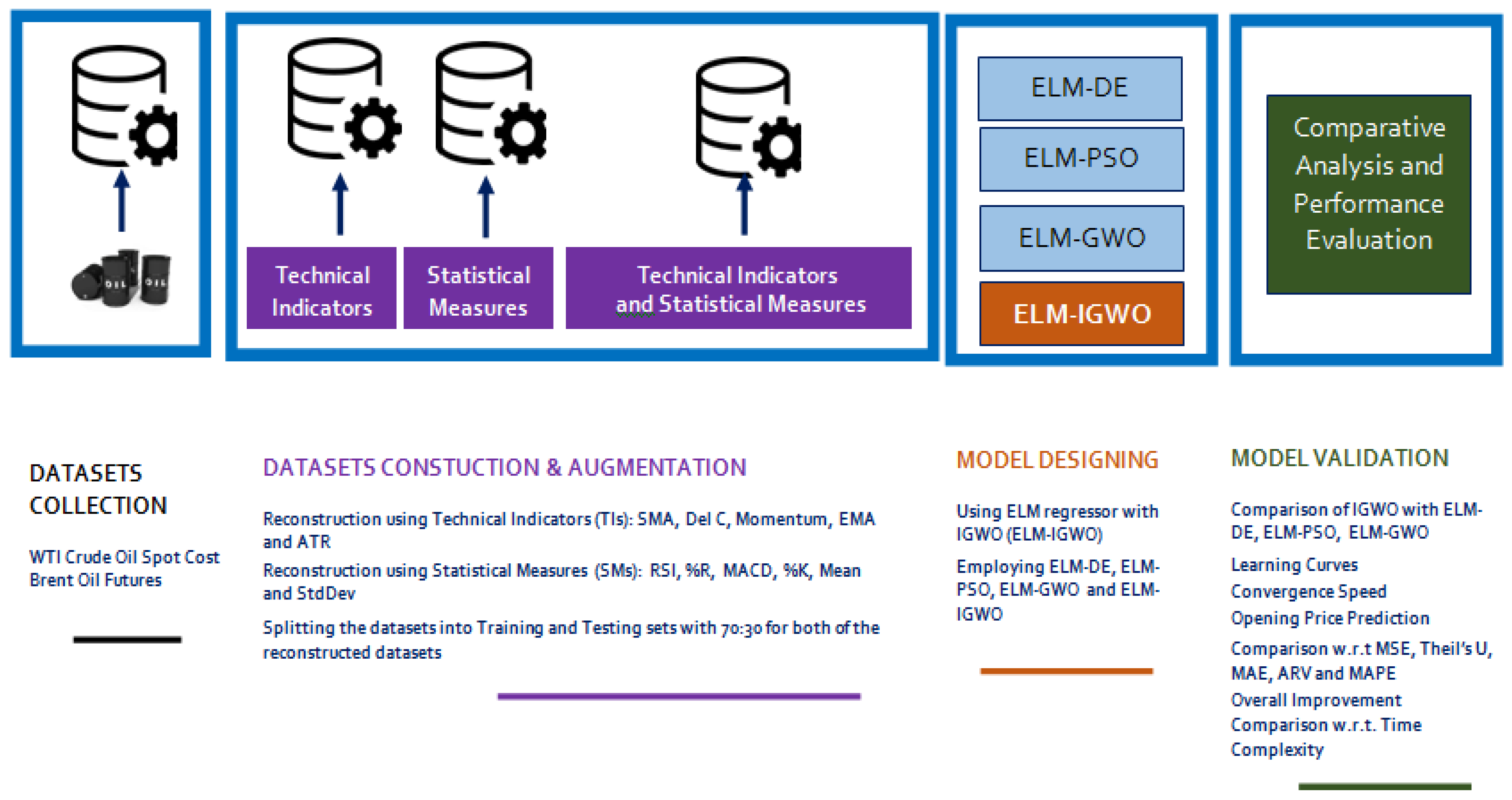
- Two datasets, the WTI crude oil and the Brent future oil datasets [48,51], were experimented on and were used to expand the model’s feasibility by augmenting the original crude oil datasets with a few technical indicators (Tis) and statistical measures (SMs) to increase the dimensionality of the original datasets [52,53]. These were finally given as inputs into the proposed ELM–IGWO crude oil forecasting model.
- (f).
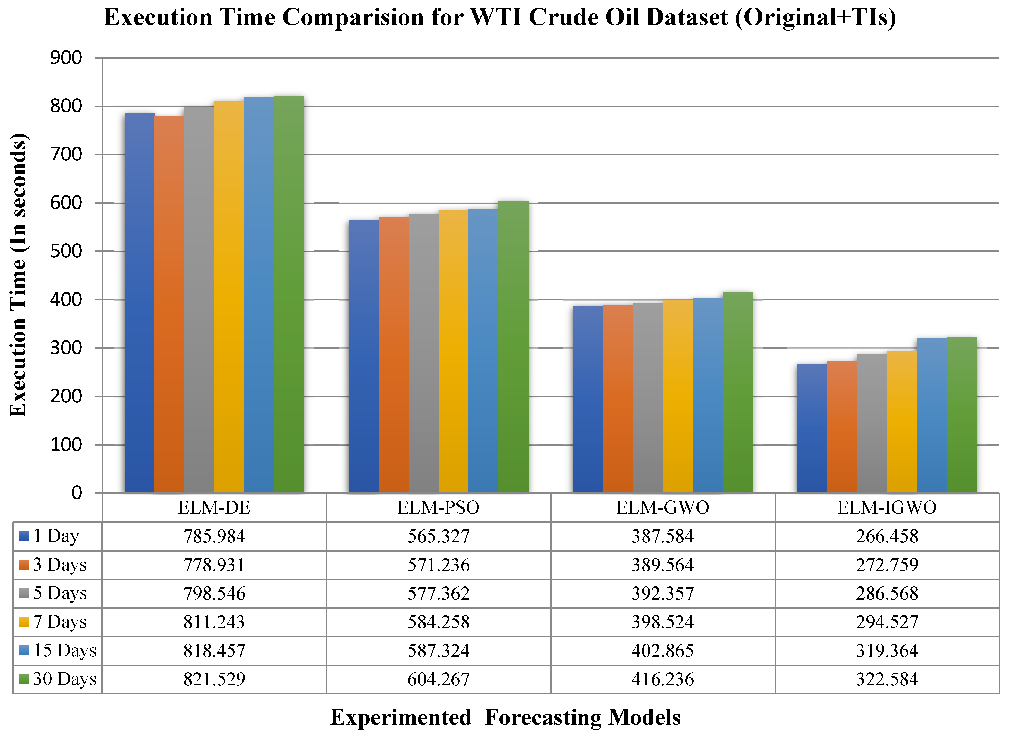
- The proposed forecasting model is compared based on mean squared error (MSE) with other hybrid ELM-based forecasting models such as ELM–DE, ELM–PSO, and ELM–GWO to validate the superiority of the results obtained.
- (g).
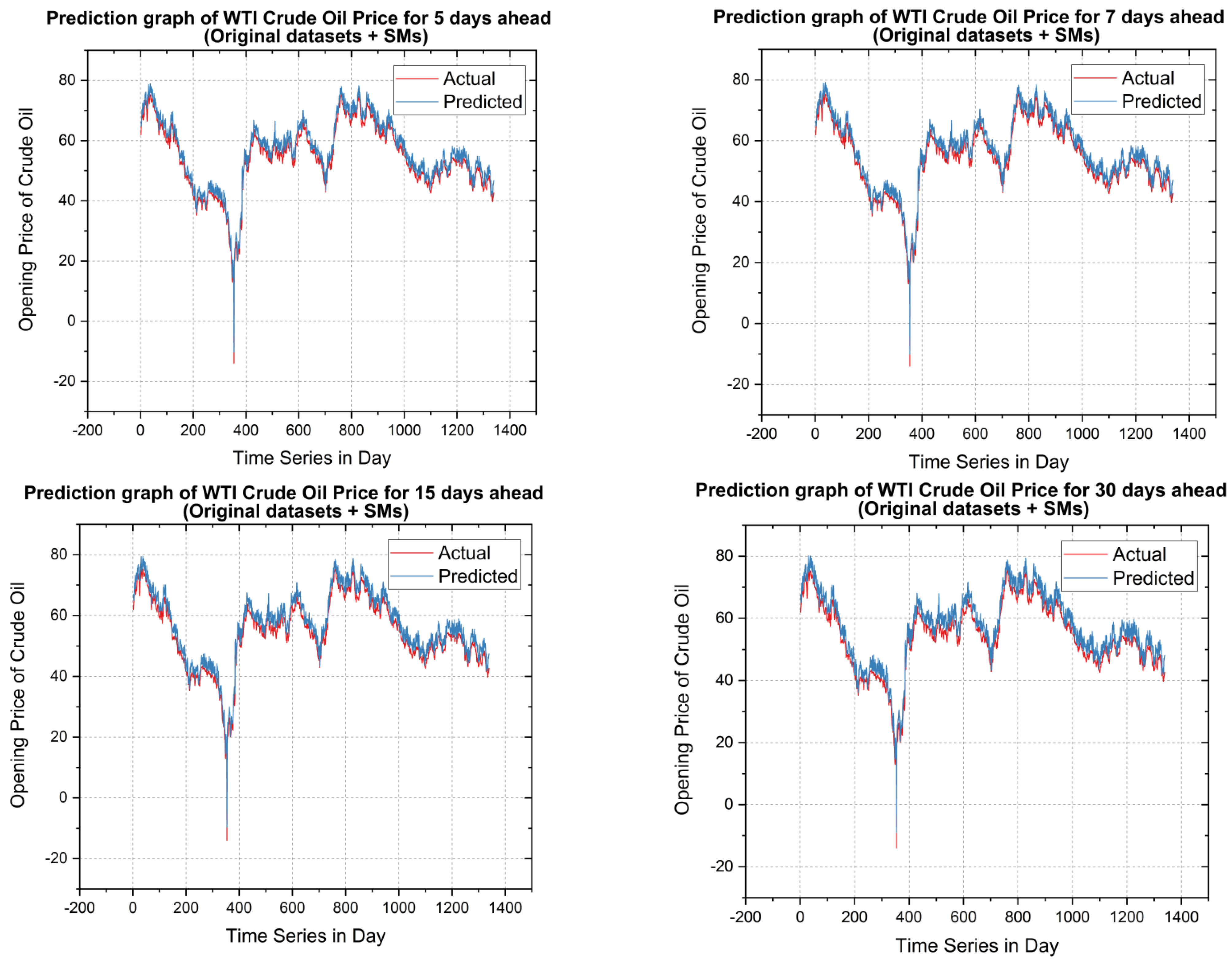
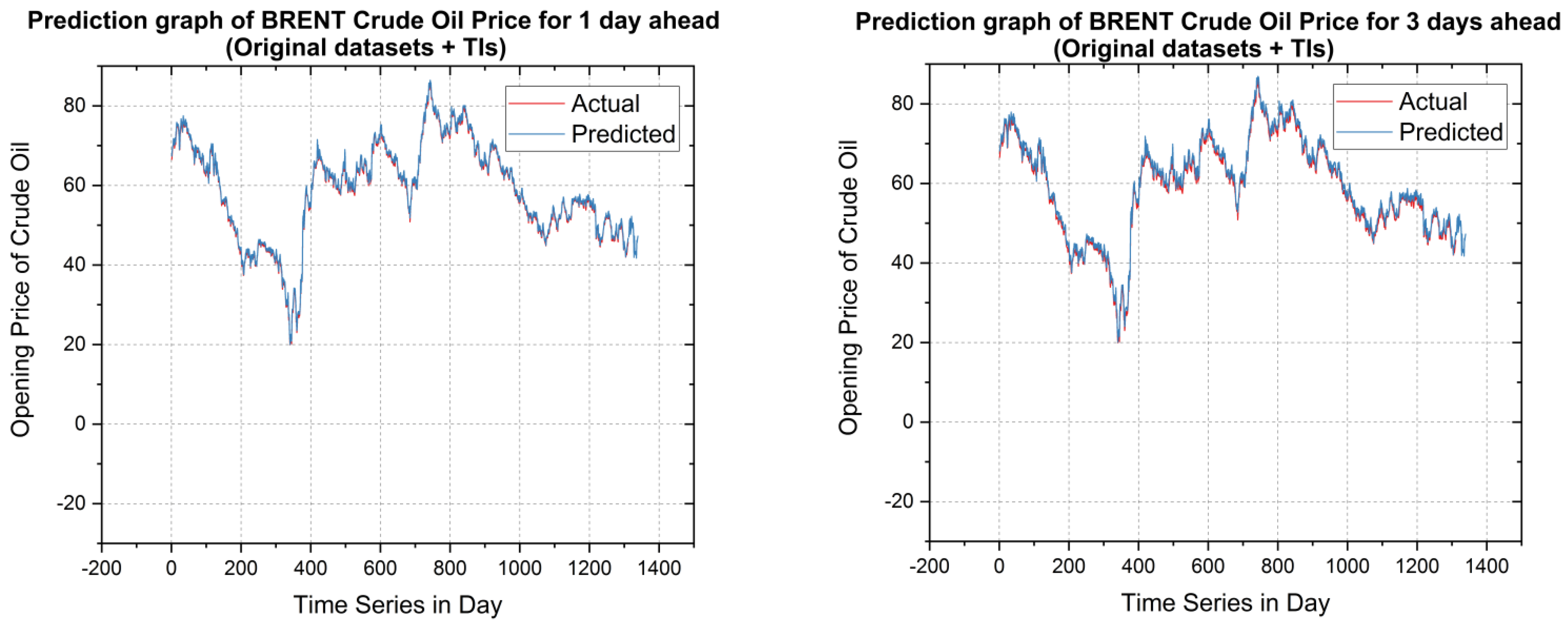
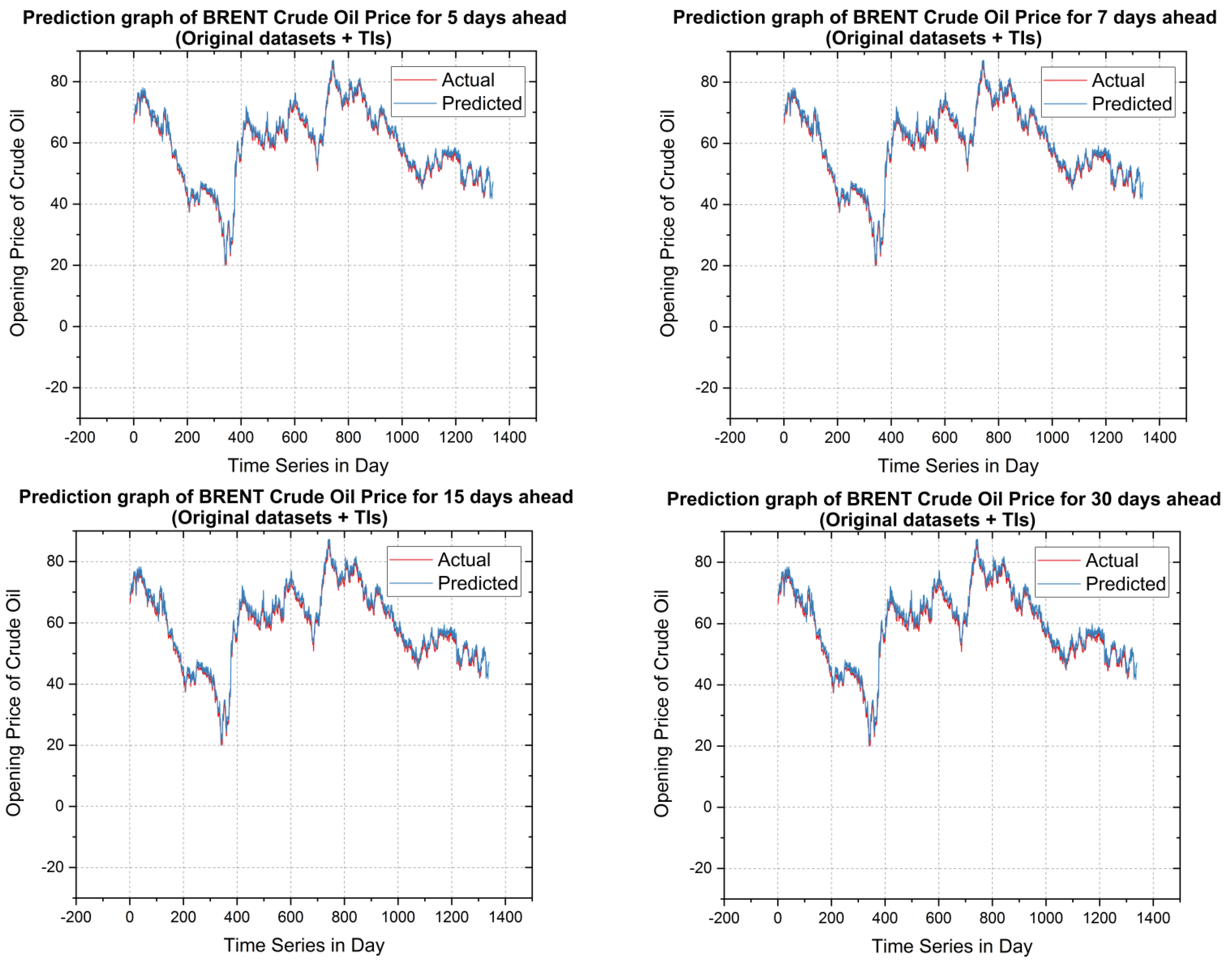
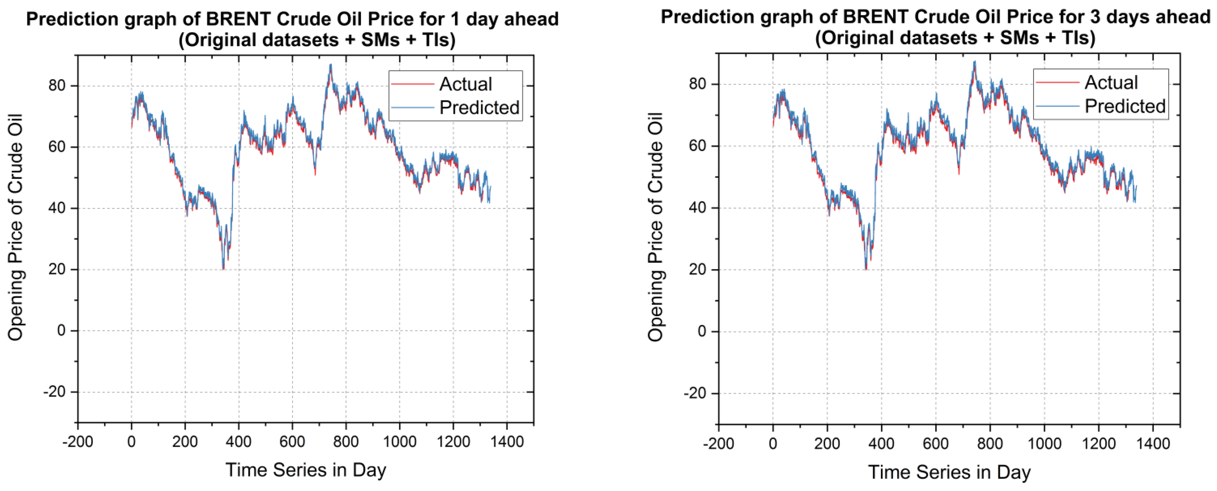
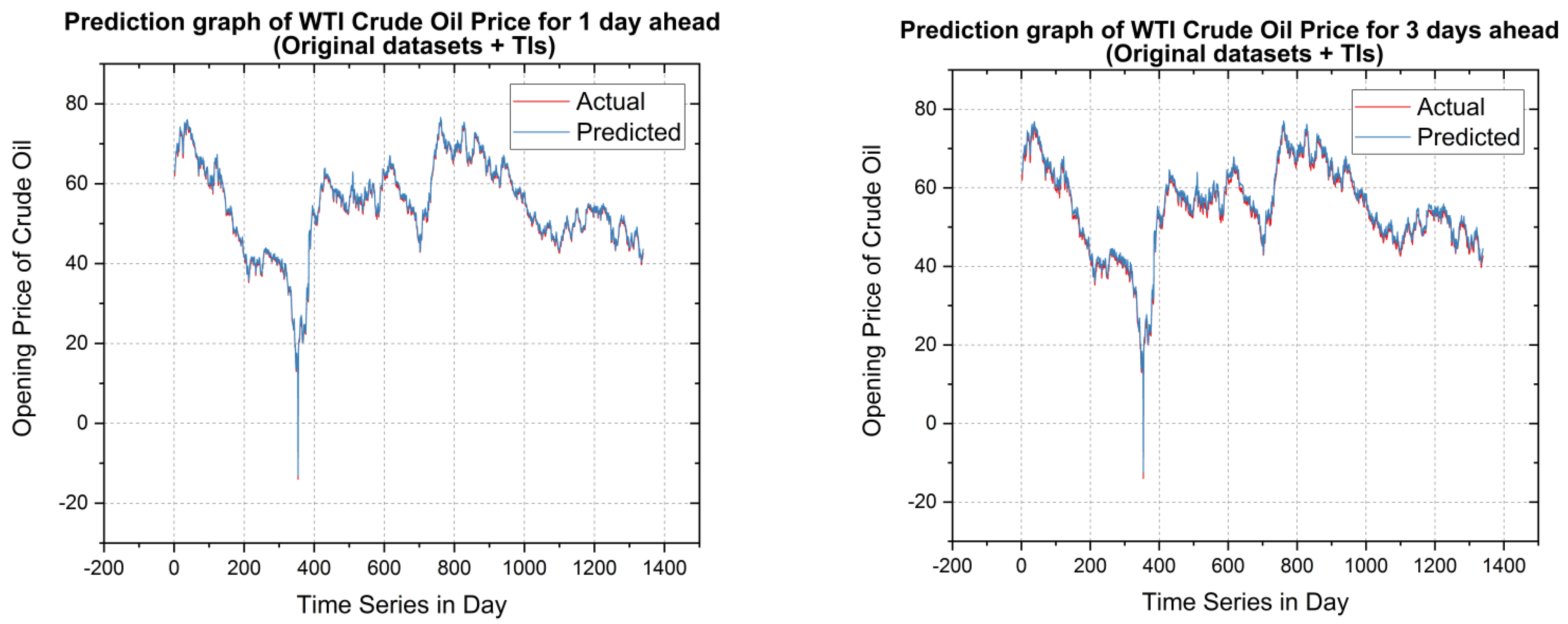
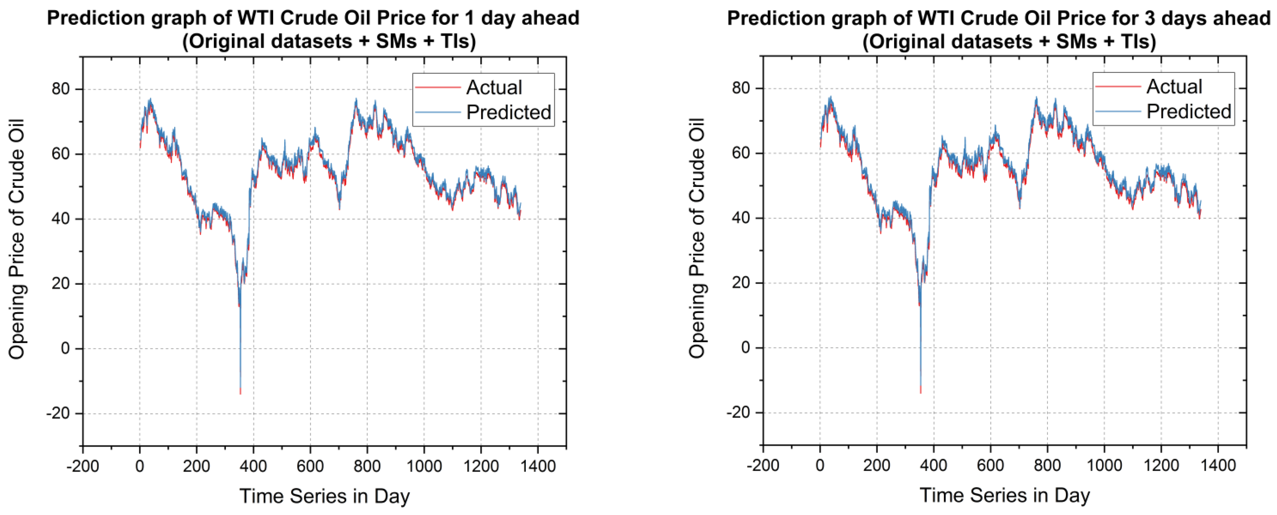
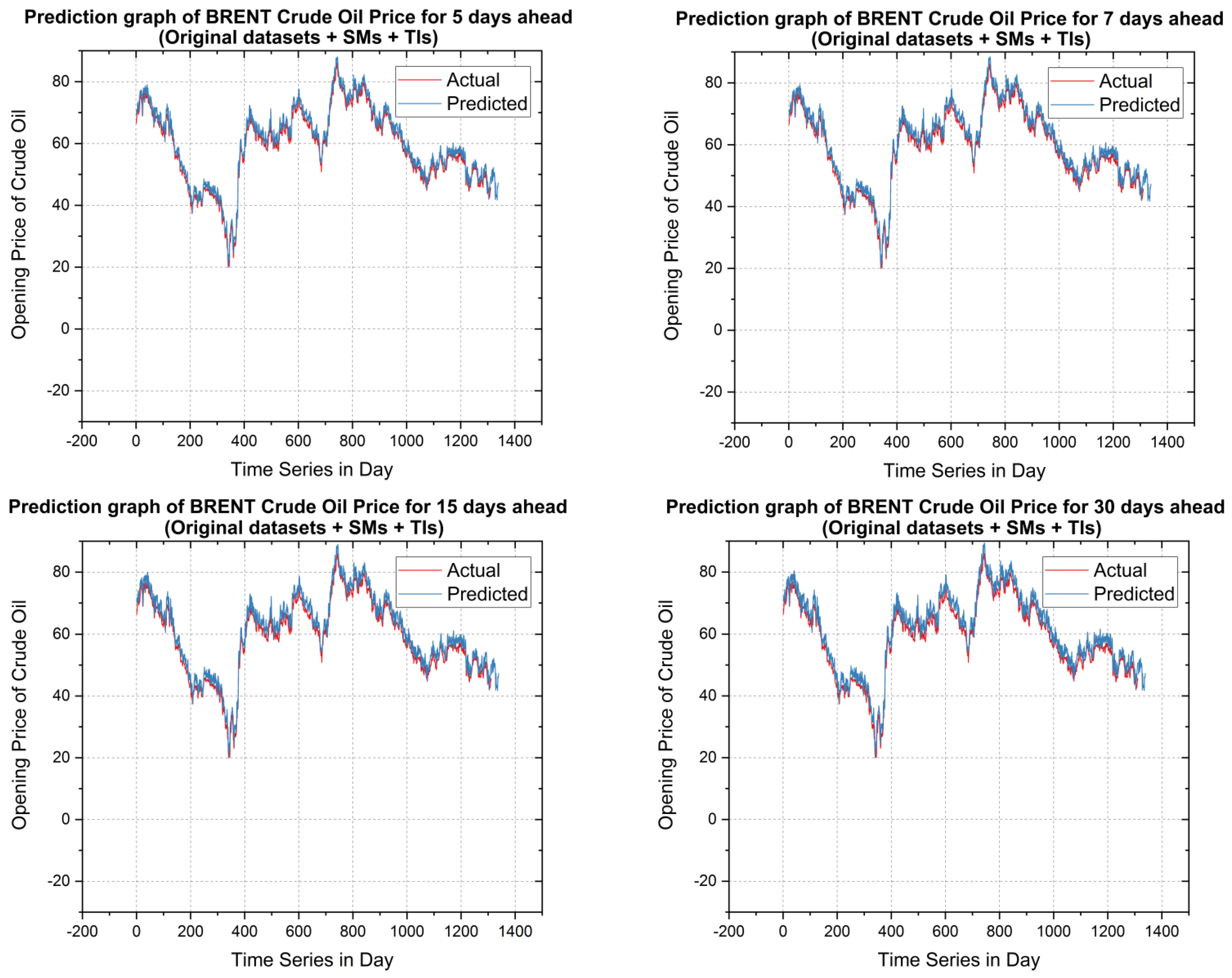
- The forecasting ability of the proposed model is established based on actual price vs. predicted price for both datasets for the three combinations of the augmented form of datasets such as original dataset +Tis, original dataset +SMs, and original dataset + Tis + SMs.
- (h).
- Finally, the model’s validation was performed based on MSE, Theil’s U, mean absolute error (MAE), average relative variance (ARV) and mean absolute percentage error (MAPE), and comparison based on CPU time utilization (in seconds) [53].
2. The Literature Review
3. Methodologies Adopted
3.1. Extreme Learning Machine (ELM)
3.2. Differential Evolution (DE)
3.3. Particle Swarm Optimization (PSO)
3.4. Standard GWO Algorithm
- (a).
- Enclosure stage: In this stage, they initially circle the prey after the wolf determines the situation of their prey. Numerically it can be presented using Equations (1) and (2). The distance between the prey and the wolf is represented by , whereas the position of the prey and the wolf after the tth iteration is represented by and respectively. The coefficient factors are illustrated in Equations (2) and (3), respectively.
- (b).
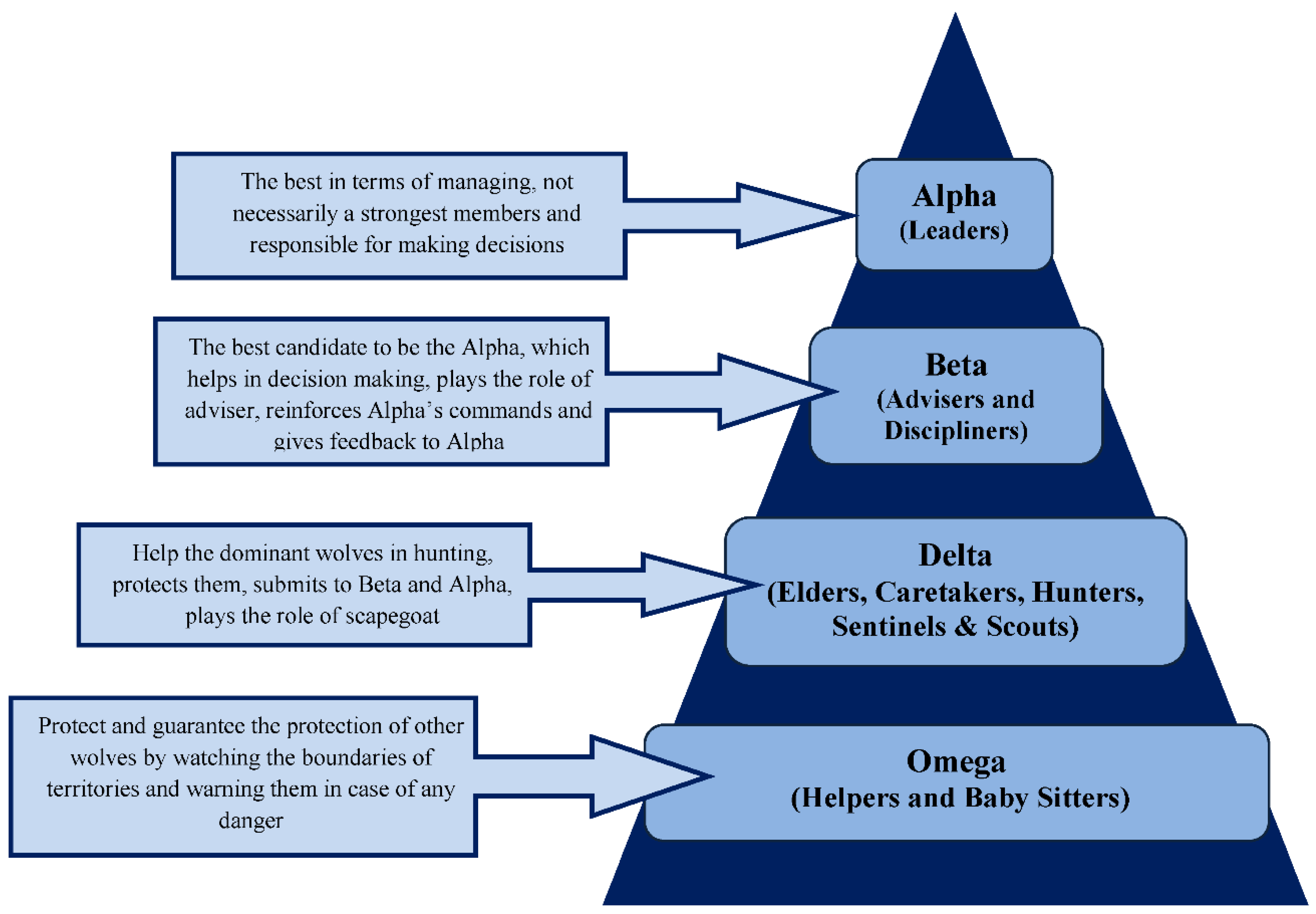
- Hunting stage: During this stage, the wolf will rapidly discover the situation of the prey and quest for the prey. At the point when the wolf discovers the situation of the prey, the wolves alpha, beta, and delta have a specific comprehension of the situation of the prey and expect w to move toward the situation of the prey. This is the prey cycle of wolves. After the attack stage is finished, the alpha wolf leads wolves beta and delta to chase down their prey. During the time spent hunting, the situation of individual wolves will move with the getaway of the prey. Where represent the current positions of wolves alpha, beta, and delta as mentioned in Equations (6)–(8), respectively, and indicates the current grey wolf position. are random vectors and the location of the wolf was updated using Equation (9).
3.5. Improved Grey Wolf Optimizer (IGWO)
- (a)
- Mutation Operation
- (b)
- Crossover Operation
- (c)
- Selection Operation
- (a).
- The strength of the wolves with respect to fitness value is measured by keeping the number of wolves fixed in a wolf pack and the concept says the wolf with the largest fitness value is chosen as the better one.
- (b).
- In this way, at each iteration, the fitness values of the wolves are sorted in ascending order thereby eliminating the wolves with a larger fitness value, and random new wolves are generated matching the number of wolves eliminated.
- (c).
- It can be observed that, when the numbers of wolves with a high fitness value are large, that leads to generating the same large number of new wolves and this type of case leads to slow convergence speed because of large search space. Similarly, if the fitness value is chosen to be too small, the diversity of the population is not guaranteed, which results in the inability of exploring new solution spaces. Therefore, the authors have proposed to have a random fitness value.
- (d).
- In this work, the fitness value was chosen to be between the range using Equation (16), where the total number of wolves is represented as n, and the wolf updating scaling parameter is termed as .
- (1)
- Creating the population of grey wolves by defining the factors such as , , and for a randomly generated wolf location .
- (2)
- Determining each wolf’s fitness and, based on the fitness value, defining the best three wolves as alpha, beta, and delta, respectively.
- (3)
- Making necessary adjustments and updating the positions of the other wolves, i.e., the w wolf, according to Equations (5)–(11).
- (4)
- The evolution of the proposed algorithm is carried out based on constructing a variation factor, using alpha, beta, and delta as described in Equation (12). After the crossover and selection operations, choosing a fit animal to be the next generation’s wolf, selecting the top three of them, and defining them as alpha, beta, and delta, in that order.
- (5)
- Sorting the wolves’ fitness values by eliminating the wolves with the highest fitness value and creating random R wolves using Equation (16).
- (6)
- Making necessary changes to factors , , and using Equations (3)–(5).
- (7)
- Determining the alpha’s position and fitness value if the termination condition is satisfied. If optimal position is not obtained, go back to step one (2).
4. Experimentation and Result Analysis
4.1. Model Description
4.2. Parameters Considered
4.3. Data Description and Data Augmentation
5. Result Analysis
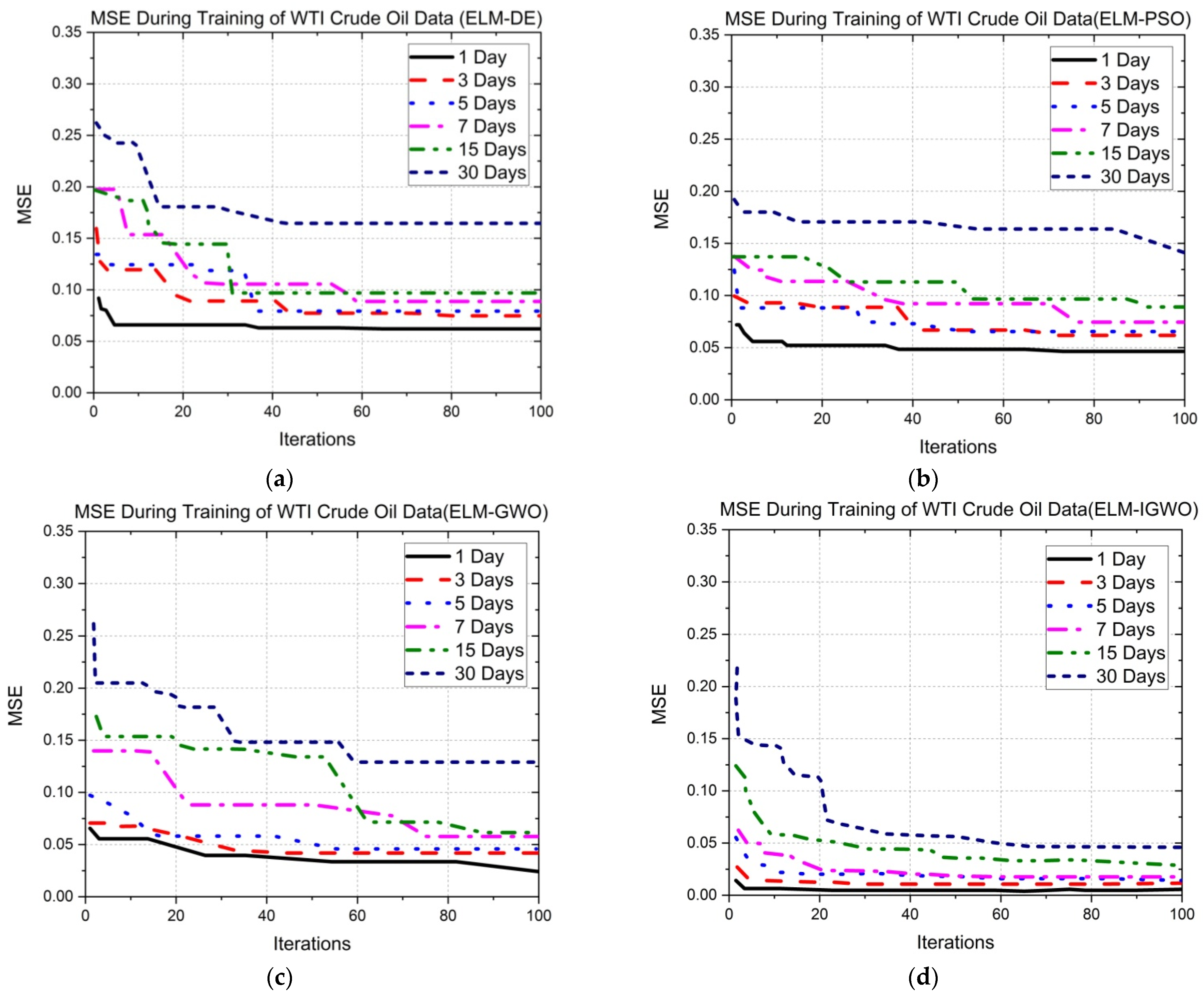
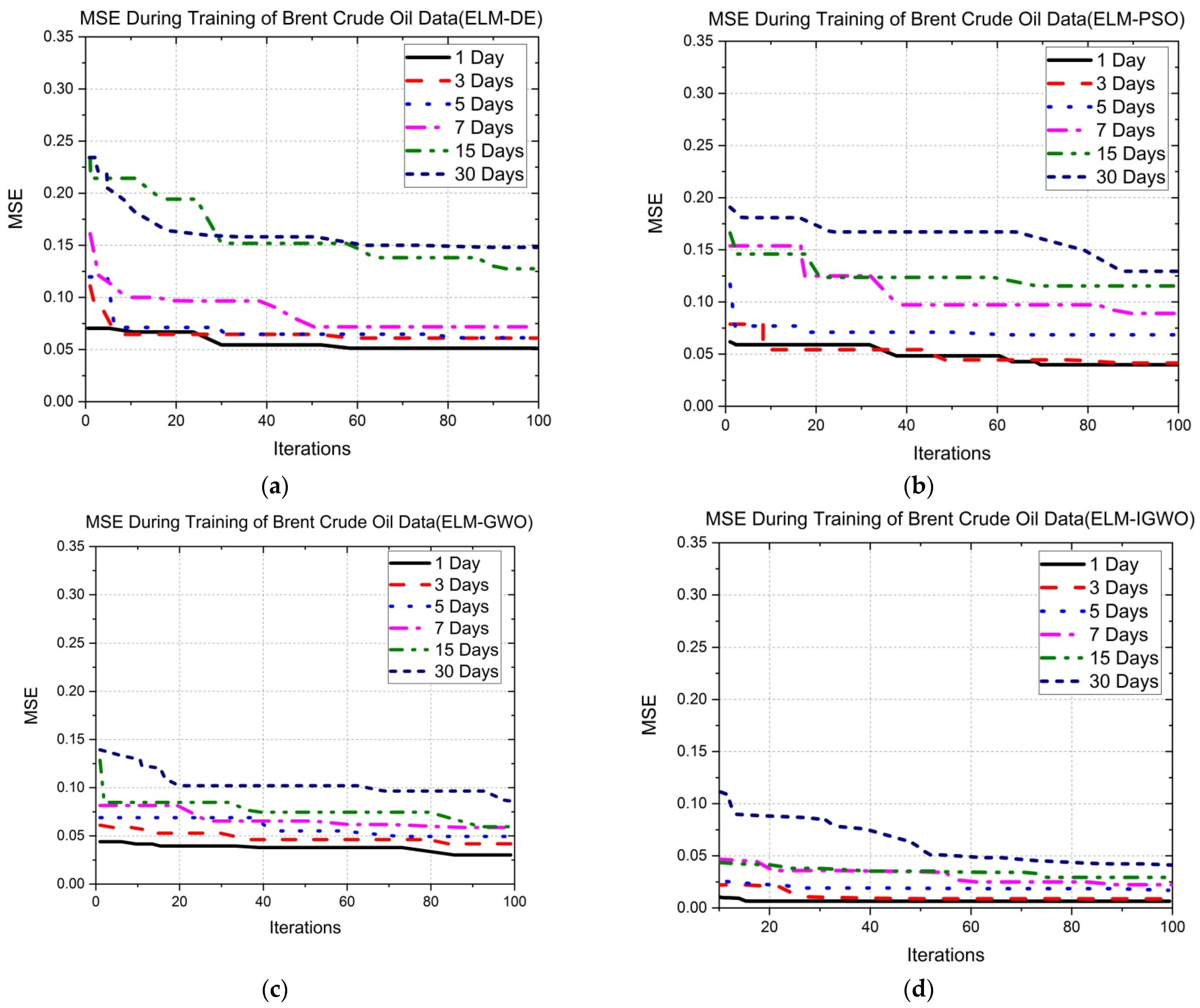
5.1. Description and Analysis of Error Convergence Graphs
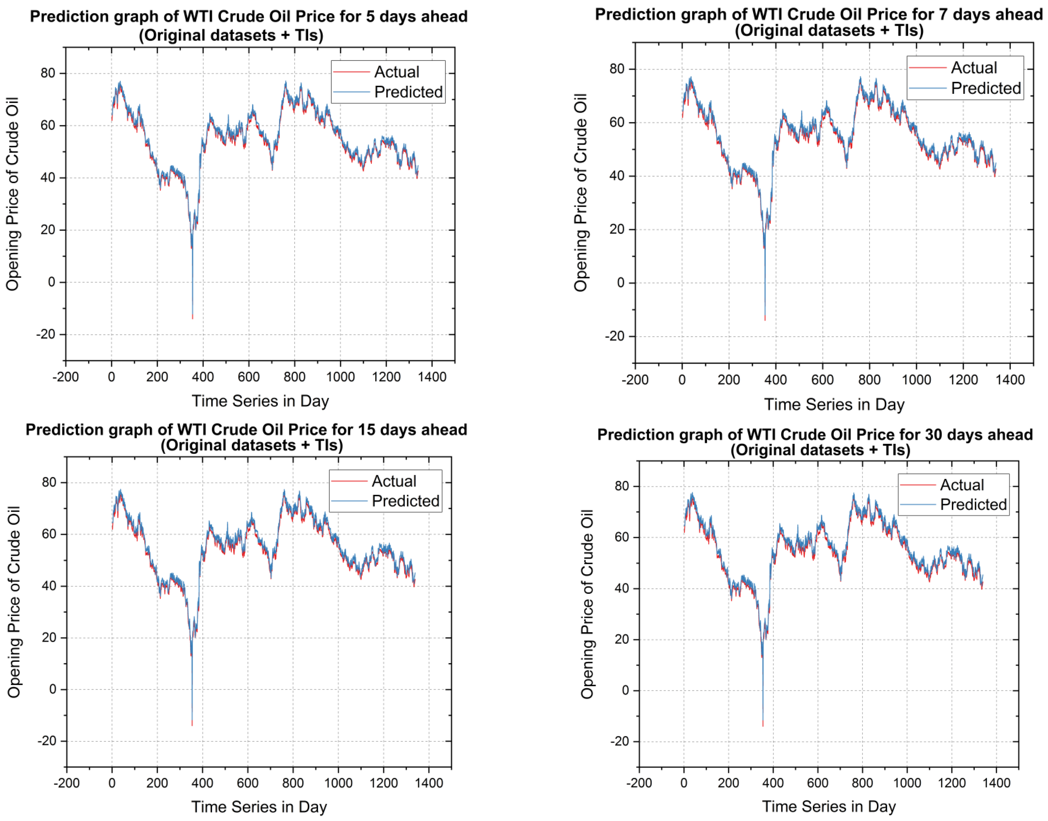
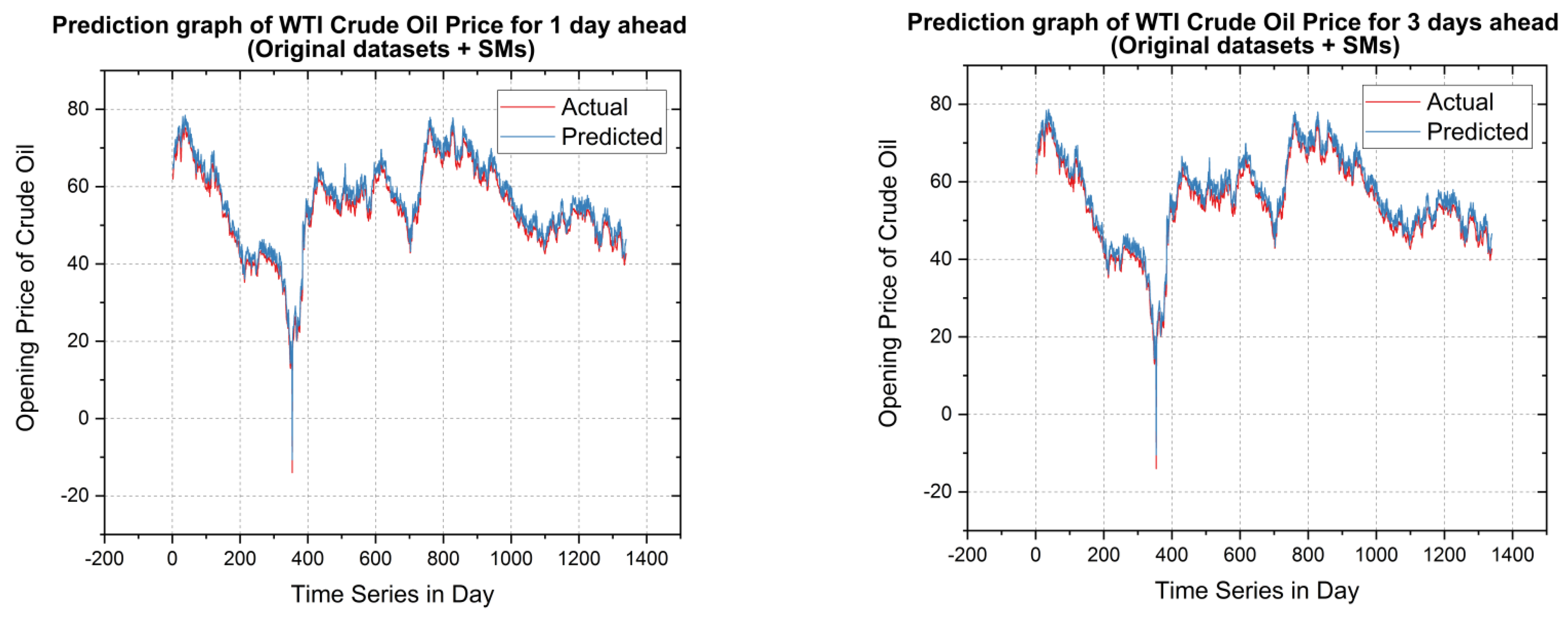
5.2. Forecasting Results and Discussions
5.3. Validation and Discussion
6. Conclusions and Future Scope
Author Contributions
Funding
Institutional Review Board Statement
Informed Consent Statement
Data Availability Statement
Conflicts of Interest
Nomenclatures
| ARMA | Autoregressive Moving Average |
| ARIMA | Autoregressive Integrated Moving Average |
| GARCH | Generalized Autoregressive Conditional Heteroscedastic |
| EGARCH | Exponential Generalized Autoregressive Conditional Heteroscedastic |
| GJR–GARCH | Glosten–Jagannathan–Runkle GARCH |
| AI | Artificial Intelligence |
| ML | Machine Learning |
| SVM | Support Vector Machine |
| BPNN | Back-Propagation Neural Networks |
| ELM | Extreme Learning Machine |
| ACO | Ant Colony Optimization |
| PSO | Particle Swarm Optimization |
| ABC | Artificial Bee Colony |
| CS | Cuckoo Search |
| DE | Differential Evolution |
| GWO | Grey Wolf Optimization |
| IGWO | Improved Grey Wolf Optimization |
| SOF | Survival Of Fittest |
| WTI | West Texas Intermediate |
| TIs | Technical Indicators |
| SMs | Statistical Measures |
| MSE | Mean Square Error |
| MAE | Mean Absolute Error |
| ARV | Average Relative Variance |
| MAPE | Mean Absolute Percentage Error |
| GA | Genetic Algorithm |
| VAR | Value At Risk |
| VMD | Variational Mode Decomposition |
| FPA | Flower Pollination Algorithm |
| DTW | Dynamic Time Warping |
| MIDAS | Mixed Data Sampling |
| CNN | Convolutional Neural Network |
| RSBL | Random Sparse Bayesian Learning |
| GARCH-M | GARCH with Long Memory |
| SMA | Simple Moving Average |
| EMA | Exponential Moving Average |
| ATR | Average True Range |
| RSI | Relative Strength Index |
| MACD | Moving Average Convergence Divergence |
| %K | Stochastic Oscillator |
| StdDev | Standard Deviation |
References
- Ahmad, M.I. Modelling and forecasting Oman Crude Oil Prices using Box-Jenkins techniques. Int. J. Trade Glob. Mark. 2012, 5, 24–30. [Google Scholar] [CrossRef]
- Morana, C. A semiparametric approach to short-term oil price forecasting. Energy Econ. 2001, 23, 325–338. [Google Scholar] [CrossRef]
- Sadorsky, P. Modeling and forecasting petroleum futures volatility. Energy Econ. 2001, 23, 325–338. [Google Scholar] [CrossRef]
- Weng, F.; Zhang, H.; Yang, C. Volatility forecasting of crude oil futures based on a genetic algorithm regularization online extreme learning machine with a forgetting factor: The role of news during the COVID-19 pandemic. Resour. Policy 2021, 73, 102148. [Google Scholar] [CrossRef] [PubMed]
- Monsef, A.; Hortmani, A.; Hamzeh, K. Prediction of Oil Price using ARMA Method for Years 2003 to 2011. Int. J. Acad. Res. Account. Financ. Manag. Sci. 2013, 3, 235–247. [Google Scholar]
- Xiang, Y.; Zhuang, X.H. Application of ARIMA model in short-term prediction of international crude oil price. Adv. Mater. Res. 2013, 798, 979–982. [Google Scholar] [CrossRef]
- Zhao, C.L.; Wang, B. Forecasting crude oil price with an autoregressive integrated moving average (ARIMA) model. In Fuzzy Information & Engineering and Operations Research & Management; Springer: Berlin/Heidelberg, Germany, 2014; pp. 275–286. [Google Scholar]
- Wu, F.; Cattani, C.; Song, W.; Zio, E. Fractional ARIMA with an improved cuckoo search optimization for the efficient Short-term power load forecasting. Alex. Eng. J. 2020, 59, 3111–3118. [Google Scholar] [CrossRef]
- Mohammadi, H.; Su, L. International evidence on crude oil price dynamics: Applications of ARIMA-GARCH models. Energy Econ. 2010, 32, 1001–1008. [Google Scholar] [CrossRef]
- Agnolucci, P. Volatility in crude oil futures: A comparison of the predictive ability of GARCH and implied volatility models. Energy Econ. 2009, 31, 316–321. [Google Scholar] [CrossRef]
- Maitra, S. GARCH Processes & Monte-Carlo Simulations for Crude-Oil Prediction. Available online: https://www.researchgate.net/publication/335977950_GARCH_Processes_Monte-Carlo_Simulations_for_Crude-Oil_Prediction (accessed on 16 March 2022).
- Hou, A.; Suardi, S. A nonparametric GARCH model of crude oil price return volatility. Energy Econ. 2012, 34, 618–626. [Google Scholar] [CrossRef]
- Wang, Y.; Wu, C. Forecasting energy market volatility using GARCH models: Can multivariate models beat univariate models? Energy Econ. 2012, 34, 2167–2181. [Google Scholar] [CrossRef]
- Wang, S.Y.; Yu, L.; Lai, K.K. A novel hybrid AI system framework for crude oil price forecasting. Lect. Notes Comput. Sci. 2004, 3327, 233–242. [Google Scholar]
- Ding, Y. A novel decompose-ensemble methodology with AIC-ANN approach for crude oil forecasting. Energy 2018, 154, 328–336. [Google Scholar] [CrossRef]
- Chai, J.; Lu, Q.; Hu, Y.; Wang, S.; Lai, K.K.; Liu, H. Analysis and Bayes statistical probability inference of crude oil price change point. Technol. Forecast. Soc. Chang. 2018, 126, 271–283. [Google Scholar] [CrossRef]
- Fan, L.; Pan, S.; Li, Z.; Li, H. An ICA-based support vector regression scheme for forecasting crude oil prices. Technol. Forecast. Soc. Chang. 2016, 112, 245–253. [Google Scholar]
- Xie, W.; Yu, L.; Xu, S.; Wang, S. A new method for crude oil price forecasting based on support vector machines. In Proceedings of the International Conference on Computational Science, Reading, UK, 28–31 May 2006; Springer: Berlin/Heidelberg, Germany, 2006; pp. 444–451. [Google Scholar]
- Ahmed, R.A.; Shabri, A.B. Daily crude oil price forecasting model using AIMA, generalized autoregressive conditional heteroscedastic and support vector machines. Am. J. Appl. Sci. 2014, 11, 425–432. [Google Scholar] [CrossRef]
- Nayak, R.K.; Mishra, D.; Rath, A.K. A Naı¨ve SVM-KNN based stock market trend reversal analysis for Indian benchmark indices. Appl. Soft Comput. 2015, 35, 670–680. [Google Scholar] [CrossRef]
- Gupta, N.; Nigam, S. Crude Oil Price Prediction using Artificial Neural Network. Procedia Comput. Sci. 2020, 170, 642–647. [Google Scholar] [CrossRef]
- Li, M.B.; Huang, G.B.; Saratchandran, P.; Sundararajan, N. Fully complex extreme learning machine. Neurocomputing 2005, 68, 306–314. [Google Scholar] [CrossRef]
- Yu, L.; Dai, W.; Tang, L. A novel decomposition ensemble model with extended extreme learning machine for crude oil price forecasting. Eng. Appl. Artif. Intell. 2016, 47, 110–121. [Google Scholar] [CrossRef]
- Wang, J.; Athanasopoulos, G.; Hyndman, R.; Wang, S. Crude oil price forecasting based on internet concern using an extreme learning machine. Int. J. Forecast. 2018, 34, 665–677. [Google Scholar] [CrossRef]
- Azadeh, A.; Asadzadeh, S.M.; Mirseraji, G.H.; Saberi, M. An emotional learningneuro-fuzzy inference approach for optimum training and forecasting of gas consumption estimation models with cognitive data. Technol. Forecast. Soc. Chang. 2015, 91, 47–63. [Google Scholar] [CrossRef]
- Escribano, Á.; Wang, D. Mixed random forest, cointegration, and forecasting gasoline prices. Int. J. Forecast. 2021, 37, 1442–1462. [Google Scholar] [CrossRef]
- Uthayakumar, J.; Metawa, N.; Shankar, K.; Lakshmanaprabu, S.K. Financial crisis prediction model using ant colony optimization. Int. J. Inf. Manag. 2020, 50, 538–556. [Google Scholar]
- Pan, M.; Li, C.; Gao, R.; Huang, Y.; You, H.; Gu, T.; Qin, F. Photovoltaic power forecasting based on a support vector machine with improved ant colony optimization. J. Clean. Prod. 2020, 277, 123948. [Google Scholar] [CrossRef]
- Ghanbari, A.; Kazemi, S.; Mehmanpazir, F.; Nakhostin, M.M. A Cooperative Ant Colony Optimization-Genetic Algorithm approach for construction of energy demand forecasting knowledge-based expert systems. Knowl.-Based Syst. 2013, 39, 194–206. [Google Scholar] [CrossRef]
- Wang, P.C.; Shoup, T.E. A poly-hybrid PSO optimization method with intelligent parameter adjustment. Adv. Eng. Softw. 2011, 42, 555–565. [Google Scholar] [CrossRef]
- Xu, X.; Ren, W. A hybrid model of stacked autoencoder and modified particle swarm optimization for multivariate chaotic time series forecasting. Appl. Soft Comput. 2021, 116, 108321. [Google Scholar] [CrossRef]
- Zhang, T.; Tang, Z.; Wu, J.; Du, X.; Chen, K. Multi-step-ahead crude oil price forecasting based on two-layer decomposition technique and extreme learning machine optimized by the particle swarm optimization algorithm. Energy 2021, 229, 120797. [Google Scholar] [CrossRef]
- Houssein, E.H.; Gad, A.G.; Hussain, K.; Suganthan, P.N. Major Advances in Particle Swarm Optimization: Theory, Analysis, and Application. Swarm Evol. Comput. 2021, 63, 100868. [Google Scholar] [CrossRef]
- Larrea, M.; Porto, A.; Irigoyen, E.; Barragán, A.J.; Andújar, J.M. Extreme learning machine ensemble model for time series forecasting boosted by PSO: Application to an electric consumption problem. Neurocomputing 2021, 452, 465–472. [Google Scholar] [CrossRef]
- Yang, X.; Yuan, J.; Yuan, J.; Mao, H. An improved WM method based on PSO for electric load forecasting. Expert Syst. Appl. 2010, 37, 8036–8041. [Google Scholar] [CrossRef]
- Wang, J.; Wang, Z.; Li, X.; Zhou, H. Artificial bee colony-based combination approach to forecasting agricultural commodity prices. Int. J. Forecast. 2019, 38, 21–34. [Google Scholar] [CrossRef]
- Cuong-Le, T.; Minh, H.-L.; Khatir, S.; Wahab, M.A.; Mirjalili, S.; Tran, M.T. A novel version of Cuckoo search algorithm for solving optimization problems. Expert Syst. Appl. 2021, 186, 115669. [Google Scholar] [CrossRef]
- Wang, L.; Hu, H.; Ai, X.-Y.; Liu, H. Effective electricity energy consumption forecasting using echo state network improved by differential evolution algorithm. Energy 2018, 153, 801–815. [Google Scholar] [CrossRef]
- Opara, K.R.; Arabas, J. Differential Evolution: A survey of theoretical analyses. Swarm Evol. Comput. 2019, 44, 546–558. [Google Scholar] [CrossRef]
- Neri, F.; Tirronen, V. Recent Advances in Differential Evolution: A survey and Experimental Analysis. Artif. Intell. Rev. 2010, 33, 61–106. [Google Scholar] [CrossRef]
- Das, S.; Mullick, S.S.; Suganthan, P.N. Recent advances in differential evolution—An updated survey. Swarm Evol. Comput. 2016, 27, 1–30. [Google Scholar] [CrossRef]
- Mirjalili, S.; Mirjalili, S.M.; Lewis, A. Grey wolf optimizer. Adv. Eng. Softw. 2014, 69, 46–61. [Google Scholar] [CrossRef] [Green Version]
- Rajakumar, R.; Sekaran, K.; Hsu, C.-H.; Kadry, S. Accelerated grey wolf optimization for global optimization problems. Technol. Forecast. Soc. Chang. 2021, 169, 120824. [Google Scholar] [CrossRef]
- Altan, A.; Karasu, S.; Zio, E. A new hybrid model for wind speed forecasting combining long short-term memory neural network, decomposition methods and grey wolf optimizer. Appl. Soft Comput. 2021, 100, 106996. [Google Scholar] [CrossRef]
- Tikhamarine, Y.; Souag-Gamane, D.; Ahmed, A.N.; Kisi, O.; El-Shafie, A. Improving artificial intelligence models accuracy for monthly streamflow forecasting using grey Wolf optimization (GWO) algorithm. J. Hydrol. 2020, 582, 124435. [Google Scholar] [CrossRef]
- Ma, X.; Mei, X.; Wu, W.; Wu, X.; Zeng, B. A novel fractional time delayed grey model with Grey Wolf Optimizer and its applications in forecasting the natural gas and coal consumption in Chongqing China. Energy 2019, 178, 487–507. [Google Scholar] [CrossRef]
- Wang, J.-S.; Li, S.-X. An Improved Grey Wolf Optimizer Based on Differential Evolution and Elimination Mechanism. Sci. Rep. 2019, 9, 7181. [Google Scholar] [CrossRef] [Green Version]
- Chai, J.; Xing, L.-M.; Zhou, X.-Y.; Zhang, Z.G.; Li, J.-X. Forecasting the WTI crude oil price by a hybrid-refined method. Energy Econ. 2018, 71, 114–127. [Google Scholar] [CrossRef]
- Ruble, I.; Powell, J. The Brent-WTI spread revisited: A novel approach. J. Econ. Asymmetries 2021, 23, e00196. [Google Scholar] [CrossRef]
- Mastroeni, L.; Mazzoccoli, A.; Quaresima, G.; Vellucci, P. Decoupling and recoupling in the crude oil price benchmarks: An investigation of similarity patterns. Energy Econ. 2021, 94, 105036. [Google Scholar] [CrossRef]
- Available online: https://in.investing.com/commodities/crude-oil-historical-statistics (accessed on 30 December 2021).
- Available online: https://www.ig.com/en/trading-strategies/10-trading-indicators-every-trader-should-know-190604 (accessed on 2 January 2022).
- Lai, T.L.; Xing, H. Statistical Models and Methods for Financial Markets; Springer: New York, NY, USA, 2008. [Google Scholar]
- Nademi, A.; Nademi, Y. Forecasting crude oil prices by a semiparametric Markov switching model: OPEC, WTI, and Brent cases. Energy Econ. 2018, 74, 757–766. [Google Scholar] [CrossRef]
- de Albuquerquemello, V.P.; de Medeiros, R.K.; da Nobrega Besarria, C.; Maia, S.F. Forecasting crude oil price: Does exist an optimal econometric model? Energy 2018, 155, 578–591. [Google Scholar] [CrossRef]
- Debnath, K.B.; Mourshed, M. Forecasting methods in energy planning models. Renew. Sustain. Energy Rev. 2018, 88, 297–325. [Google Scholar]
- Tang, L.; Yu, L.; Wang, S.; Li, J.P.; Wang, S.Y. A novel hybrid ensemble learning paradigm for nuclear energy consumption forecasting. Appl. Energy 2012, 93, 432–443. [Google Scholar] [CrossRef]
- Guo, X.; Li, D.; Zhang, A. Improved Support Vector Machine Oil Price Forecast Model Based on Genetic Algorithm Optimization Parameters. AASRI Procedia 2012, 1, 525–530. [Google Scholar] [CrossRef]
- Zhao, L.; Cheng, L.; Wan, Y.; Zhang, H.; Zhang, Z. A VAR-SVM model for crude oil price forecasting. Int. J. Glob. Energy Issues 2015, 38, 126–144. [Google Scholar] [CrossRef]
- Jianwei, E.; Bao, Y.; Ye, J. Crude oil price analysis and forecasting based on variational mode decomposition and independent component analysis. Phys. A Stat. Mech. Appl. 2017, 484, 412–427. [Google Scholar]
- Xiao, Y.; Xiao, J.; Lu, F.; Wang, S. Ensemble ANNs-PSO-GA Approach for Day-ahead Stock E-exchange Prices Forecasting. Int. J. Comput. Intell. Syst. 2014, 7, 272–290. [Google Scholar] [CrossRef] [Green Version]
- Alfi, A.; Modares, H. System identification and control using adaptive particle swarm optimization. Appl. Math. Model. 2011, 35, 1210–1221. [Google Scholar] [CrossRef]
- Yang, X.S. Flower pollination algorithm for global optimization. In Proceedings of the International Conference on Unconventional Computing and Natural Computation, Orléans, France, 3–7 September 2012; Springer: Berlin/Heidelberg, Germany, 2012; pp. 240–249. [Google Scholar]
- Chiroma, H.; Khan, A.; Abubakar, A.I.; Saadi, Y.; Hamza, M.F.; Shuib, L.; Gital, A.Y.; Herawan, T. A new approach for forecasting OPEC petroleum consumption based on neural network train by using flower pollination algorithm. Appl. Soft Comput. 2016, 48, 50–58. [Google Scholar] [CrossRef]
- He, K.; Tso, G.K.; Zou, Y.; Liu, J. Crude oil risk forecasting: New evidence from multiscale analysis approach. Energy Econ. 2018, 76, 574–583. [Google Scholar] [CrossRef]
- Czudaj, R.L. Heterogeneity of beliefs and information rigidity in the crude oil market: Evidence from survey data. Eur. Econ. Rev. 2022, 143, 104041. [Google Scholar] [CrossRef]
- Dutta, A.; Bouri, E.; Saeed, T. News-based equity market uncertainty and crude oil volatility. Energy 2021, 222, 119930. [Google Scholar] [CrossRef]
- He, K.; Zou, Y. Crude oil risk forecasting using mode decomposition based model. Procedia Comput. Sci. 2022, 199, 309–3142. [Google Scholar] [CrossRef]
- Chen, Z.; Ye, Y.; Li, X. Forecasting China’s crude oil futures volatility: New evidence from the MIDAS-RV model and COVID-19 pandemic. Resour. Policy 2021, 75, 102453. [Google Scholar] [CrossRef] [PubMed]
- Zhao, Y.; Zhang, W.; Gong, X.; Wang, C. A novel method for online real-time forecasting of crude oil price. Appl. Energy 2021, 303, 117588. [Google Scholar] [CrossRef]
- Wu, B.; Wang, L.; Lv, S.-X.; Zeng, Y.-R. Effective crude oil price forecasting using new text-based and big-data-driven model. Measurement 2021, 168, 108468. [Google Scholar] [CrossRef]
- Li, T.; Qian, Z.; Deng, W.; Zhang, D.; Lu, H.; Wang, S. Forecasting crude oil prices based on variational mode decomposition and random sparse Bayesian learning. Appl. Soft Comput. 2021, 113, 108032. [Google Scholar] [CrossRef]
- Abdollahi, H. A novel hybrid model for forecasting crude oil price based on time series decomposition. Appl. Energy 2020, 267, 115035. [Google Scholar] [CrossRef]
- Lin, L.; Jiang, Y.; Xiao, H.; Zhou, Z. Crude oil price forecasting based on a novel hybrid long memory GARCH-M and wavelet analysis model. Phys. AStat. Mech. Appl. 2020, 543, 123532. [Google Scholar] [CrossRef]
- Deng, S.; Xiang, Y.; Fu, Z.; Wang, M.; Wang, Y. A hybrid method for crude oil price direction forecasting using multiple timeframes dynamic time wrapping and genetic algorithm. Appl. Soft Comput. 2019, 82, 105566. [Google Scholar] [CrossRef]


| Source | Year | Objective(s) | Model(s) Adopted | Finding(s) | Pros | Cons |
|---|---|---|---|---|---|---|
| Kaijian Hea et al. [68] | 2022 | To calculate the value at risk factor of crude oil | Md VaR based risk forecasting model using multiple mode decomposition model and Quantile regression neural network | The proposed model is used to calculate VaR by using a semi-parametric data-driven approach for both normal market and transient market conditions. | The VaR estimated by the proposed MD VaR model gives more reliability and accuracy | The complex risk structure has not been analyzed. |
| Zhonglu Chen et al. [69] | 2022 | To predict the realized volatility of China’s crude oil futures | Mixed data sampling (MIDAS) modeling framework: MIDAS–RV Model | In this work, both the jump and leverage effects are used to predict the RV of Chinese crude oil futures, where jump is used for the short-term and leverage effects used for long-term prediction. | The model is robust and economic. During the COVID-19 epidemic, the model is used to guide the investors as well as market participants. It also reduces the investment risks | - |
| Yuan Zhao et al. [70] | 2021 | To improve the accuracy of online real-time price forecasting for crude oil. | PSO–VMD algorithm and the and PVMD–SVM–ARMA model | In this paper, an improved variational mode decomposition is used with PSO to optimize the parameters and then the proposed hybrid model established the characteristics of sub-sequences, and the interval prediction model is constructed with the combination of point prediction model and Bootstrap sampling and finally, these can be used as a predictor to predict the online real-time price of crude oil. | The model poses flexibility and accuracy, which can give more information for people working with oil. | The method used for prediction is only mint for small samples and short-term periods. |
| Binrong Wu et al. [71] | 2021 | Effective crude oil price predicting | Convolutional neural network (CNN), VMD | In order to predict the crude oil price, here, a combined approach of Google trends and news text information was proposed which applied the following methodologies: relationship investigation, deep learning techniques, and decomposition techniques. | This approach provides satisfactory accuracy for crude oil price prediction. Google trends and news text information can promote each other. | The Google trends used in this approach are a complex process. Except for VMD, no other decomposition techniques were used to improve the accuracy. |
| Taiyong Li et al. [72] | 2021 | To reduce the complexity rises in Crude oil price forecasting | VMD and random sparse Bayesian learning (RSBL) VMD–RSBL | Here the authors have introduced random samples and random lags (features) into SBL and built an individual forecasting model with the combination of VMD and RSBL. | The proposed VMD–RSBL model is effective and efficient | The method is not applied for multivariate price forecasting |
| Hooman Abdollahi [73] | 2020 | To improve the accuracy of crude oil price prediction by considering the characteristics that exist in the oil price time series | Model by hybridizing the methods such as complete ensemble empirical mode decomposition, support vector machine, particle swarm optimization, and Markov-switching generalized autoregressive conditional heteroskedasticity | The algorithm is used as an effective tool for predicting nonlinear components and both the forecasted nonlinear components and volatile components result in the reliable forecast of the oil price. | The model predicted the volatile components with appropriate accuracy and gives the best performance while forecasting the component with low volatility. | The model was not applied to forecast other energy commodities in order to prove the robustness and generalizability. |
| Ling Lin et al. [74] | 2020 | To forecast crude oil price by considering the long memory, asymmetric, heavy-tail distribution, nonlinear, and non-stationary characteristics of crude oil price. | The model combined the complex long memory GARCH-M with wavelet analysis | The model can forecast the crude oil price during periods of extreme incidents. MS–DR method and crude oil volatility are being used here to model large fluctuations within the forecasting interval. | The model proposed can provide beneficial information required for the process of forecasting and Helps the investors to determine overall trends in oil prices reduce the market risks. | - |
| Shangkun Deng et al. [75] | 2019 | To predict the changes of crude oil price, as well as execute simulated trading. | Hybrid model based on multiple timeframes dynamic time wrapping and GA is developed for direction forecasting and simulation trading | The proposed method includes four components such as; (1) Data Pre-processing, (2) Multiple timeframes DTW prediction, (3) GA parameters optimization, and (4) Prediction, trading, and evaluation | The model gives high performances in terms of hit ratio, accumulated return, and Sharpe ratio, and the results are significantly superior to that of benchmark methods. It can also provide beneficial information to investors, energy-related enterprises, and government officers engaged in policy decisions. | The model should work with short term data |
| Forecasting Models | Parameters | Values |
|---|---|---|
| ELM | Hidden Neurons | 10 |
| Weight Range | [0, 1] | |
| DE | Crossover Probability | 0.25 |
| Scaling factor range [Max, Min] | [0.2, 0.9] | |
| PSO | Search coefficient | 2.5 |
| Search coefficient | 1.3 | |
| Inertia Weight | 0.8 | |
| GWO | (Decreased linearly) | 2.0 |
| IGWO | (Decreased linearly) | 2.0 |
| Crossover probability | 0.2 | |
| Scaling factor range [Max, Min] | [0.2, 0.9] |
| Technical Indicators and Statistical Measures | Formula |
|---|---|
| Simple Moving Average (SMA) | |
| Del C | |
| Momentum | |
| Exponential Moving Average (EMA) | |
| Average True Range (ATR) | |
| Relative Strength Index (RSI) | |
| William’s %R | |
| Moving average convergence divergence (MACD) | |
| Stochastic Oscillator (%K) | |
| Mean | |
| Standard Deviation (StdDev) |
| Datasets | Total Samples | Data Range | Training Sample | Test Sample |
|---|---|---|---|---|
| WTI Crude Oil Spot Cost | 1341 | 25 July 2016 to 23 August 2021 | 940 | 401 |
| Brent Oil Futures | 1311 | 25 July 2016 to 23 August 2021 | 917 | 394 |
| No. of Days | ELM–DE | ELM–PSO | ELM–GWO | ELM–IGWO | ||||||||
|---|---|---|---|---|---|---|---|---|---|---|---|---|
| TIs | SMs | TIs and SMs | TIs | SMs | TIs and SMs | TIs | SMs | TIs and SMs | TIs | SMs | TIs and SMs | |
| 1 Day | 3.262 × 10⁻⁴ | 3.136 × 10⁻⁴ | 6.076 × 10⁻⁴ | 3.494 × 10⁻⁴ | 4.136 × 10⁻⁴ | 5.076 × 10⁻⁴ | 1.368 × 10⁻⁴ | 1.572 × 10⁻⁴ | 5.248 × 10⁻⁴ | 1.053 × 10⁻⁴ | 1.08 × 10⁻⁴ | 5.042 × 10⁻⁴ |
| 3 Days | 3.591 × 10⁻⁴ | 3.438 × 10⁻⁴ | 7.664 × 10⁻⁴ | 3.671 × 10⁻⁴ | 3.988 × 10⁻⁴ | 7.664 × 10⁻⁴ | 2.986 × 10⁻⁴ | 1.575 × 10⁻⁴ | 9.347 × 10⁻⁴ | 2.872 × 10⁻⁴ | 1.48 × 10⁻⁴ | 9.52 × 10⁻⁴ |
| 5 Days | 2.357 × 10⁻⁴ | 2.433 × 10⁻⁴ | 2.182 × 10⁻⁴ | 3.883 × 10⁻⁴ | 3.937 × 10⁻⁴ | 4.178 × 10⁻⁴ | 1.714 × 10⁻⁴ | 1.643 × 10⁻⁴ | 2.178 × 10⁻⁴ | 1.744 × 10⁻⁴ | 1.4 × 10⁻⁴ | 2.1 × 10⁻⁴ |
| 7 Days | 3.493 × 10⁻⁴ | 3.769 × 10⁻⁴ | 3.452 × 10⁻⁴ | 3.992 × 10⁻⁴ | 4.169 × 10⁻⁴ | 4.478 × 10⁻⁴ | 1.421 × 10⁻⁴ | 4.232 × 10⁻⁴ | 1.82 × 10⁻⁴ | 1.038 × 10⁻⁴ | 4.16 × 10⁻⁴ | 1.64 × 10⁻⁴ |
| 15 Days | 3.263 × 10⁻⁴ | 4.832 × 10⁻⁴ | 7.097 × 10⁻⁴ | 4.247 × 10⁻⁴ | 4.832 × 10⁻⁴ | 6.563 × 10⁻⁴ | 1.691 × 10⁻⁴ | 4.48 × 10⁻⁴ | 1.164 × 10⁻⁴ | 1.26 × 10⁻⁴ | 4.32 × 10⁻⁴ | 1.07 × 10⁻⁴ |
| 30 Days | 11.44 × 10⁻⁴ | 11.64 × 10⁻⁴ | 14.58 × 10⁻⁴ | 9.42 × 10⁻⁴ | 9.67 × 10⁻⁴ | 12.49 × 10⁻⁴ | 9.374 × 10⁻⁴ | 8.771 × 10⁻⁴ | 11.61 × 10⁻⁴ | 8.52 × 10⁻⁴ | 8.47 × 10⁻⁴ | 11.57 × 10⁻⁴ |
| No. of Days | ELM–DE | ELM–PSO | ELM–GWO | ELM–IGWO | ||||||||
|---|---|---|---|---|---|---|---|---|---|---|---|---|
| TIs | SMs | TIs and SMs | TIs | SMs | TIs and SMs | TIs | SMs | TIs and SMs | TIs | SMs | TIs and SMs | |
| 1 Day | 2.962 × 10⁻⁴ | 3.467 × 10⁻⁴ | 5.189 × 10⁻⁴ | 2.653 × 10⁻⁴ | 3.457 × 10⁻⁴ | 5.136 × 10⁻⁴ | 1.276 × 10⁻⁴ | 1.837 × 10⁻⁴ | 4.567 × 10⁻⁴ | 1.103 × 10⁻⁴ | 1.238 × 10⁻⁴ | 4.308 × 10⁻⁴ |
| 3 Days | 3.191 × 10⁻⁴ | 3.892 × 10⁻⁴ | 6.738 × 10⁻⁴ | 2.897 × 10⁻⁴ | 3.324 × 10⁻⁴ | 6.438 × 10⁻⁴ | 2.583 × 10⁻⁴ | 1.983 × 10⁻⁴ | 5.462 × 10⁻⁴ | 2.387 × 10⁻⁴ | 1.948 × 10⁻⁴ | 4.987 × 10⁻⁴ |
| 5 Days | 4.556 × 10⁻⁴ | 4.896 × 10⁻⁴ | 5.344 × 10⁻⁴ | 3.988 × 10⁻⁴ | 4.231 × 10⁻⁴ | 4.874 × 10⁻⁴ | 1.897 × 10⁻⁴ | 2.278 × 10⁻⁴ | 3.773 × 10⁻⁴ | 1.664 × 10⁻⁴ | 2.086 × 10⁻⁴ | 3.479 × 10⁻⁴ |
| 7 Days | 6.278 × 10⁻⁴ | 6.395 × 10⁻⁴ | 7.378 × 10⁻⁴ | 4.994 × 10⁻⁴ | 5.362× 10⁻⁴ | 5.436 × 10⁻⁴ | 1.354 × 10⁻⁴ | 3.256 × 10⁻⁴ | 2.321 × 10⁻⁴ | 1.203 × 10⁻⁴ | 4.325 × 10⁻⁴ | 2.089 × 10⁻⁴ |
| 15 Days | 5.839 × 10⁻⁴ | 5.852 × 10⁻⁴ | 6.997 × 10⁻⁴ | 4.667 × 10⁻⁴ | 4.875 × 10⁻⁴ | 5.573 × 10⁻⁴ | 2.479 × 10⁻⁴ | 3.988 × 10⁻⁴ | 2.658 × 10⁻⁴ | 2.263 × 10⁻⁴ | 3.132 × 10⁻⁴ | 2.019 × 10⁻⁴ |
| 30 Days | 9.563 × 10⁻⁴ | 10.187 × 10⁻⁴ | 11.158 × 10⁻⁴ | 8.347 × 10⁻⁴ | 9.246 × 10⁻⁴ | 11.473 × 10⁻⁴ | 8.894 × 10⁻⁴ | 9.093 × 10⁻⁴ | 10.568 × 10⁻⁴ | 8.224 × 10⁻⁴ | 8.787 × 10⁻⁴ | 9.588 × 10⁻⁴ |
| Methods | Theil’s U | MAE | ARV | MAPE |
|---|---|---|---|---|
| ELM–DE | 0.0014587 | 0.1356 | 0.004985 | 0.42578 |
| ELM–PSO | 0.0002784 | 0.0687 | 0.001256 | 0.12586 |
| ELM–GWO | 0.0001658 | 0.0027 | 0.000653 | 0.07842 |
| ELM–IGWO | 0.0001013 | 0.0009 | 0.000854 | 0.02967 |
Publisher’s Note: MDPI stays neutral with regard to jurisdictional claims in published maps and institutional affiliations. |
© 2022 by the authors. Licensee MDPI, Basel, Switzerland. This article is an open access article distributed under the terms and conditions of the Creative Commons Attribution (CC BY) license (https://creativecommons.org/licenses/by/4.0/).
Share and Cite
Das, A.K.; Mishra, D.; Das, K.; Mallick, P.K.; Kumar, S.; Zymbler, M.; El-Sayed, H. Prophesying the Short-Term Dynamics of the Crude Oil Future Price by Adopting the Survival of the Fittest Principle of Improved Grey Optimization and Extreme Learning Machine. Mathematics 2022, 10, 1121. https://doi.org/10.3390/math10071121
Das AK, Mishra D, Das K, Mallick PK, Kumar S, Zymbler M, El-Sayed H. Prophesying the Short-Term Dynamics of the Crude Oil Future Price by Adopting the Survival of the Fittest Principle of Improved Grey Optimization and Extreme Learning Machine. Mathematics. 2022; 10(7):1121. https://doi.org/10.3390/math10071121
Chicago/Turabian StyleDas, Asit Kumar, Debahuti Mishra, Kaberi Das, Pradeep Kumar Mallick, Sachin Kumar, Mikhail Zymbler, and Hesham El-Sayed. 2022. "Prophesying the Short-Term Dynamics of the Crude Oil Future Price by Adopting the Survival of the Fittest Principle of Improved Grey Optimization and Extreme Learning Machine" Mathematics 10, no. 7: 1121. https://doi.org/10.3390/math10071121
APA StyleDas, A. K., Mishra, D., Das, K., Mallick, P. K., Kumar, S., Zymbler, M., & El-Sayed, H. (2022). Prophesying the Short-Term Dynamics of the Crude Oil Future Price by Adopting the Survival of the Fittest Principle of Improved Grey Optimization and Extreme Learning Machine. Mathematics, 10(7), 1121. https://doi.org/10.3390/math10071121