Article

IFS-Based Image Reconstruction of Binary Images with Functional Networks

1
Department of Applied Mathematics and Computational Sciences, Universidad de Cantabria, 39005 Santander, Spain
2
Department of Information Science, Faculty of Sciences, Toho University, 2-2-1 Miyama, Funabashi 274-8510, Japan
3
Faculty of Electrical Engineering and Computer Science, University of Maribor, 2000 Maribor, Slovenia
4
R&D EgiCAD, School of Civil Engineering, Universidad de Cantabria, Avda. de los Castros 44, 39005 Santander, Spain
*
Author to whom correspondence should be addressed.
Mathematics 2022, 10(7), 1107; https://doi.org/10.3390/math10071107
Submission received: 2 March 2022 / Revised: 25 March 2022 / Accepted: 26 March 2022 / Published: 29 March 2022
(This article belongs to the Special Issue Computer Graphics, Image Processing and Artificial Intelligence)

Abstract

:
This work addresses the IFS-based image reconstruction problem for binary images. Given a binary image as the input, the goal is to obtain all the parameters of an iterated function system whose attractor approximates the input image accurately; the quality of this approximation is measured according to a similarity function between the original and the reconstructed images. This paper introduces a new method to tackle this issue. The method is based on functional networks, a powerful extension of neural networks that uses functions instead of the scalar weights typically found in standard neural networks. The method relies on an artificial network comprised of several functional networks, one for each of the contractive affine maps forming the IFS. The method is applied to an illustrative and challenging example of a fractal binary image exhibiting a complicated shape. The graphical and numerical results show that the method performs very well and is able to reconstruct the input image using IFS with high accuracy. The results also show that the method is not yet optimal and offers room for further improvement.

1. Introduction

1.1. Motivation

Fractals are exciting mathematical entities that have sparked the popular imagination and interest owing to their highly original and captivating graphical images. However, well beyond their graphical appeal, researchers have found a wide variety of applications of fractals in several fields. They have been used to produce realistic computer-generated images of plants and other organic shapes for digital movies as well as to add special effects in cinema, such as the blockbuster productions Star Trek II: The Wrath of Khan (1982), Star Wars Episode III: Revenge of the Sith (2005), Guardians of the Galaxy Vol. 2 (2017), and many other movies. Fractals have also been used to describe many physical and natural objects and phenomena, including sharp coastlines, mountain ranges, snowflakes, lightnings, forest canopy, river networks, and many others. Even some parts of our own bodies (such as our neural, respiratory, and circulatory systems, to name just a few) can be adequately represented by and analyzed with fractals. Fractal signals are used to analyze heartbeats in cardiology or identify anomalous tissues in cancer research. Fractal antennas are popular in small-size telecommunication devices, while fractal image compression is used to store images more efficiently. We can even find public exhibitions about fractal art in art galleries and museums. Other applications arise in astronomy, computer graphics and animation, biology, dynamical systems, bioinformatics, fluid dynamics, surface physics, and many other fields [1,2,3,4,5].
This wide range of applications can be partly explained by the ubiquitous nature of fractals, but also by the variety of methods used to generate them. Fractals can be obtained through Brownian motion, random walk techniques, escape-time procedures, finite subdivision rules, L-systems, as strange attractors of dynamical systems, and other techniques [1,3,5,6]. A popular method for obtaining fractal images called Iterated Function Systems (IFS) was proposed in the 1980s [7,8,9]. The method comes from the observation that any finite collection of contractive affine maps (called an IFS) on a complete metric space has one and only one compact fixed set under the action of the Hutchinson operator (see Section 2.3 for details). Such a set is called the attractor of the IFS, and its graphical representation is a fractal image (see Section 2.4 for details). Conversely, the collage theorem states that any image in 2D (in particular, binary images) can be represented by an IFS (see Section 2.6 for details). Obtaining the parameters of such IFS (including the total number of contractive functions) is called the IFS inverse problem (likewise known as an IFS-based image reconstruction). This is also the problem addressed in this paper.
There are many methods used for image reconstruction described in the literature. Most of them are based on image processing techniques; for instance, see [10]. A completely different approach to image reconstruction is given by the use of IFS. A clear advantage of this approach is that the image is encoded by a set of simple contractive maps, each represented by just six parameters. Once the IFS code of an image is obtained, the image can be efficiently stored as a collection of IFS parameters called the IFS code (see Section 3 for details). Given this IFS code, the image can be readily displayed through efficient real-time algorithms (see Section 2.4 and Section 2.5 for details). Therefore, instead of storing the image as a bitmap, it can be more efficiently represented through the IFS code. Furthermore, since the rendering of the image can be performed for any number of iterations, the image can be enlarged at will without degrading its visual quality; it is just a matter of increasing the number of iterations. In other words, the image behaves similar to a vector image but with a much lower file size. This capacity can be exploited to store a huge collection of very large images while using a relatively small memory.

1.2. Previous Work

The idea to use IFS codes to display fractal images was proposed by Barnsley in [7], based on the theoretical work on iterated function systems by Hutchinson [9]. A popular algorithm for rendering fractal images was presented in [11]. Another method for the IFS coding and rendering of fractal images was introduced in [12]. Other methods include wavelet transforms [13], gradient search [14], and moment matching [15,16,17], but they are computationally expensive and generally limited to some particular and simple examples. An interesting survey on fractal image compression is given in [18]. Although the paper is currently not updated, the reference is still valuable in demonstrating the great interest in this topic, as evidenced by the large number of previous works in the field. Unfortunately, all these methods were computationally expensive, restricting its applicability to challenging examples.
A more recent trend in the field is the application of artificial intelligence and machine learning techniques to address difficult optimization problems for which classical mathematical optimization techniques do not provide satisfactory solutions. In this regard, there have been some attempts to apply such techniques to the IFS inverse problem. This interest was motivated by the observation that this problem could be formulated as a nonlinear optimization problem. The works in [19,20,21,22,23,24] tried to obtain the IFS coding of fractal bitmap images through genetic algorithms and/or genetic programming. Other works applied evolutionary algorithms [25], bat algorithm [26], and particle swarm optimization [27,28]. Other examples of these techniques can be found in [29,30,31,32,33]. However, these methods were strongly limited in several regards. On the one hand, the methods were generally limited to the case of very few affine contractive maps (usually with a maximum of three or four functions), thus severely restricting the potential range of reconstructed images [19,25,33]. On the other hand, the methods were applied to very small input images, such as those of 64 × 64 pixels in [25] or 128 × 128 pixels in [33]. Whenever the authors tried to consider larger sizes such as 256 × 256 , the results were very poor or required an unreasonably huge number of contractive maps, such as hundreds or thousands of functions. Due to these strong limitations and the inability to achieve good results, the interest in this problem decreased substantially during the last decade, with only a few papers being published in the field. Two recent works by the authors of [34,35] addressed the IFS inverse problem for colored images. Although at first sight, the problem appears to be similar to that addressed in this paper, it is actually quite different. Since the input images in [34,35] were colored, additional color-based methods could be used to help in the search for the number of contractive maps and their parametric values. In both papers, histograms of the colored input images were computed and then combined with image clustering using the multilevel Otsu algorithm in [34] or the K-means algorithm in [35]. Obviously, these approaches cannot be applied here because our input consists exclusively of binary images.

1.3. Aim and Main Contributions of This Paper

This paper introduces a new method to solve the IFS-based image reconstruction problem in the case of binary images. Given a binary image, the goal is to compute the parameters of an IFS so that its attractor would yield an image that is similar to the input image according to some similarity metrics. The method is based on the application of functional networks, a powerful extension of the classical artificial neural networks. Two important features of the functional networks are that the weights in neural networks are now replaced (fully or partially) by functions, and that the activation functions of the neurons do not need to be the same for all neurons. Thanks to these new features, the functional networks are more flexible than the neural networks and can replicate the mathematical structure of a given problem more faithfully. This ability is successfully employed in this work through an artificial network comprised of several functional networks (as many as the number of contractive functions) that replicate the mathematical structure of the contractive affine functions of an IFS. In this way, the IFS-based image reconstruction is solved by computing all IFS parameters as the solutions of an optimization problem—that of minimizing the distance between the original image and the reconstructed image, as measured by a chosen similarity error function. The performance of the method is assessed by its application to an example of a fractal image exhibiting a complex shape.
The main contributions of this paper can be summarized as follows:
  • Novelty: As discussed above, a major feature of the functional networks is their ability to replicate the mathematical structure of any given problem. This feature is not present in other artificial intelligence paradigms such as neural networks, where the activation function belongs to some prescribed families of functions unrelated to the problem at hand, and the learning process is driven by the scalar weights. On the contrary, the functional networks can learn the mathematical formulation of any functional expression by using functions of one or several variables instead of weights. This makes them very well-suited for problems such as the one addressed in this paper. In spite of these powerful features, to the best of our knowledge, no previous work reported so far in the literature has applied functional network formalism to the IFS inverse problem. This work opens a promising line of research towards the application of this methodology to the reconstruction of binary images through IFS.
  • Generality: The method does not impose any constraints on the input binary image. As a result, it is very general and can be applied to any binary image and for any number of contractive functions. The limitations of previous methods with regard to the number of contractive maps and/or the size of the input images can be avoided with our proposal.
  • Good performance: As discussed in Section 6, the method performs quite well, being able to reproduce the input image with good visual quality. The numerical results of the comparative analysis in Section 6.4 also show that this method outperforms other alternative approaches described in the literature, such as neural networks, simulated annealing, genetic algorithms, and the firefly algorithm.
  • Low computational complexity: The order of complexity of the method is comparable to state-of-the-art techniques in artificial intelligence such as neural networks, genetic algorithms, or particle swarm optimization. Furthermore, the method requires fewer operations than these alternative methods.

1.4. Structure of This Paper

This paper is organized as follows: Section 2 introduces the main mathematical concepts and definitions required to follow this work. A brief discussion about artificial neural networks and their extension, functional networks (the approach used in this work), is given in Section 3. Then, the problem addressed in this paper is discussed in Section 4, while Section 5 describes our method in detail. The computational experiments and results are discussed in Section 6. The paper closes in Section 7 with the main conclusions and some future work in the field.

2. Mathematical Concepts and Definitions

This section provides the basic mathematical concepts and definitions required to follow the paper. The interested reader is referred to [1,4,9,36] for further information.

2.1. Contractive Maps and Banach Fixed-Point Theorem

Definition 1.
Let ( S , d ) be a metric space, where S is a non-empty set, and d a distance defined on S. A contractive map h on ( S , d ) is a function h : S S holding that there is a real number 0 C < 1 , such that for any pair x , y S :
d ( h ( x ) , h ( y ) ) C . d ( x , y )
An important result due to Polish mathematician Stefan Banach is the Banach fixed-point theorem, also called contractive mapping theorem, first stated in 1922.
Theorem 1
(Banach fixed-point theorem). Let ( S , d ) be a complete metric space, and h a contractive map h : S S . Then, h has a unique fixed-point p in S, that is, h ( p ) = p . Moreover, given any x 0 S , the sequence { x n } n N given by x n = h ( x n 1 ) , n N , n 1 converges to p, i.e., lim n x n = p .

2.2. Iterated Function Systems

Definition 2.
Let ( D , Δ ) be a complete metric space, with D R n , and Δ being a distance on D . An IFS (iterated function system) is a finite collection of functions { F 1 , F 2 , , F N } , where each function F i is a contractive affine map on D according to Definition 1. Note that the IFS can be represented as the tuple: { D ; F 1 , F 2 , , F N } .
The focus in this paper is on 2D binary images; therefore, we consider the case n = 2 . This means that the contractive affine maps F i are applied onto the set D R 2 . Let d 2 denote the Euclidean distance. We consider the space ( R 2 , d 2 ) , which is a complete metric space. In this case, any contractive affine map F k can be represented mathematically as follows:
ζ 1 * ζ 2 * = F k ζ 1 ζ 2 = ξ 11 k ξ 12 k ξ 21 k ξ 22 k . ζ 1 ζ 2 + τ 1 k τ 2 k
This expression can be written in vector notation as: F k ( Θ ) = A k . Θ + b k , where A k is a 2 × 2 matrix representing the rotation and scaling operations, and b k is a two-dimensional vector representing the translations. Because F k is a contractive map, the eigenvalues of A k , denoted as λ 1 k , λ 2 k , hold: | λ j k | < 1 . Furthermore, s k = | d e t ( A k ) | < 1 . The graphical interpretation of this property is that the map F k shrinks the Euclidean distance between any two points.
From Equation (1), we can see that the contractive affine map F k is uniquely represented by the set of parameters { ξ 11 k , ξ 12 k , ξ 21 k , ξ 22 k , τ 1 k , τ 2 k } , which are called IFS parameters of function F k . Consequently, the IFS { D ; F 1 , F 2 , , F N } is fully characterized by the collection of parameters { ξ i j k , τ i k } i , j = 1 , 2 ; k = 1 , , N , which is called the IFS code.

2.3. Hausdorff Metric and Hutchinson Operator

Definition 3.
Let C S ( D ) denote the set of all compact subsets of D . The Hausdorff metric H on C S ( D ) is mathematically defined as follows:
H ( R , S ) = m a x d H ( R , S ) , d H ( S , R )
where d H ( R , S ) = max x R min y S d 2 ( x , y ) .
The Heine–Borel theorem states that for any L D R 2 with the Euclidean distance d 2 , L is a compact set if and only if L is a closed and bounded set. We remark that the 2D binary images in this work are closed and bounded and are hence compact subsets of the Euclidean space R 2 .
Theorem 2.
The space ( C S ( D ) , H ) , where C S ( D ) is the set of all compact subsets of D and H is the Hausdorff metric on C S ( D ) , is also a complete metric space.
Proof. 
This theorem is a consequence of the fact that ( R 2 , d 2 ) is a complete metric space. See [1] for a proof. □
Definition 4.
It is possible to define a transformation on C S ( D ) , known as the Hutchinson operator and denoted by H , as follows:
H ( B ) = k = 1 N F k ( B ) B C S ( D )
This operator defines the joint action of all contractive maps F k .
Theorem 3.
Since all the F k are contractive maps in ( R 2 , d 2 ) , H is also a contractive function in ( C S ( D ) , H ) .
Proof. 
See [9] for a proof. □
Corollary 1.
According to the Banach fixed-point theorem, H has a unique fixed point H ( A ) = A , which is called the attractor of the IFS. This fixed-point set A is a fractal image.

2.4. Rendering the IFS Attractor

There are several ways of rendering the attractor of an IFS given by contractive maps { F 1 , F 2 , , F N } [6]. A popular approach is given by the probabilistic algorithm, where each contractive map F k is assigned a probability p k > 0 , such that k = 1 N p k = 1 . To this aim, an initial compact set B 0 D is considered, and then one of the contractive maps F k of the IFS is randomly chosen at iteration j with probability p k to yield B j = F k ( B j 1 ) . This process is repeated iteratively for the resulting set. It can be proved that lim j B j = A . This implies that this iterative procedure can be successfully applied to display the attractor [1,37]. Note that the initial set B 0 in this algorithm can be any non-empty compact set. However, because all the maps F k are contractive, it is convenient to select B 0 as a single point for better computational efficiency.

2.5. The Chaos Game

It is worth mentioning that the attractor of the IFS is determined exclusively by its IFS code, while the probabilities p k do not play any role in defining the attractor. However, they play an important role in the computational performance of rendering the attractor. This leads to the problem of determining good values for the probabilities. Several methods have been described in the literature to solve this issue [3,38]. The most common and popular method is called the chaos game, also known as Barnsley’s algorithm. The method proportionally assigns a probability value p k to the area described by the contractive map F k , which is in turn proportional to its contractivity factor s k = | d e t ( A k ) | = | ξ 11 k . ξ 22 k ξ 12 k . ξ 21 k | . Once all contractivity factors are calculated, they are normalized to obtain the probabilities as follows:
p k = s k j = 1 N s j ; k = 1 , , N .
This method can be improved by using the multifractal formalism to derive optimal values for the probabilities [37]. However, this optimal procedure is more difficult to achieve and unnecessary for the goals of this paper. Therefore, in what follows, we always apply the chaos game method to compute for the probabilities.

2.6. The Collage Theorem

An important result of IFS that has a relevant application to images is the collage theorem, first presented in [8].
Theorem 4
(Collage Theorem). Given an IFS, { D ; F 1 , , F N } , with a contractivity factor 0 < s < 1 given by s = max k = 1 , , N s k , and B being a non-empty compact subset B C S ( D ) , if
H B , H ( B ) = H B , k = 1 N F k ( B ) ϵ
for some ϵ 0 , then
H B , A ϵ 1 s
where A is the attractor of the IFS. This is equivalent to saying that:
H B , A 1 1 s H B , k = 1 N F k ( B ) .
Proof. 
See [1,8] for a proof. □
Intuitively, the collage theorem means that for any given image B , it is possible to find an IFS whose attractor A can approximate B accurately, where the approximation accuracy is measured in terms of the Hausdorff metric. However, the theorem says nothing about how to obtain such an IFS. This is the problem addressed in this paper, which will be described in detail in Section 4.

3. Functional Networks

3.1. Artificial Neural Networks

Artificial neural networks (ANNs) are one of the most popular and widely used artificial intelligence techniques. Their popularity has increased dramatically in recent years as ANNs are fundamental components of many algorithms for deep learning. ANNs are inspired by the biological structure of the brain of humans and other mammals. Similar to their biological counterparts, ANNs consist of a collection of individual processing units called neurons, which are arranged in different layers, including an input layer, an output layer, and one or several layers called hidden layers, which connect the input and output layers. It is important to point out that the information generally flows forward from the input layer to the output layer. Neurons are connected through signals replicating the synaptic signals observed in biological neural networks. In ANNs, these signals are affected by scalar values called weights, which are modified dynamically depending on the input used during the training phase. These weights determine the importance of any given variable, with the effect of larger ones contributing more significantly to the output as compared to other (lower) values. In this way, the weights play a significant role in the learning process. Additionally, the neurons can have a threshold value, also called a bias. Whenever the output of an individual neuron is above the specified threshold value, the neuron is activated, and its output is sent to neurons of the same or next layers of the network. Otherwise, no data are transferred from that neuron to the rest of the network.
To process the information, each neuron N j receives some inputs x i from the neurons of previous layers, then it computes the linear combination i = 1 m w i j x i + b , where x i is the input coming from neuron N i , w i j is the weight of the connection between the neurons N i and N j , in this specific order, and b denotes the bias. Each neuron also has an activation function, such that the output of the neuron is modulated by this function. The activation function is usually nonlinear to allow the network to learn and perform more complicated tasks. Typical activation functions are the sigmoid function, hyperbolic tangent, the ReLU function, and the softmax function.
Finally, an important aspect of ANNs is the network architecture, which determines how many layers are created, how the different neurons are arranged in such layers, and how the neurons are interconnected. There are many possible architectures (feedforward, self-organizing maps, radial basis function, recurrent, convolutional, modular, etc.), although they are mostly grouped into some specific categories, which depend on the criteria used to classify them. These different architectures are usually designed for different purposes. For more details on ANNs see, for instance, [39].

3.2. Functional Networks

Although artificial neural networks have shown remarkable ability to solve several problems, they are also severely limited in many aspects. For instance, ANNs are strongly limited to describing complex mathematical expressions as they use the same activation function for all the neurons. Furthermore, the activation function always has a single variable, so multivariate problems cannot be properly represented. Finally, the connections between neurons are associated with (strictly) scalar weights, once again dramatically restricting the flexibility of ANNs.
All the above-mentioned drawbacks can be solved by using functional networks, which were first introduced in [40]. Functional networks have been successfully applied to many problems in the scientific and engineering domains [41,42,43]. In short, functional networks are a powerful and versatile extension of the traditional artificial neural networks in which the scalar weights are replaced by functions. Such functions must not necessarily be univariate; instead, functions of several variables can also be used. These new features confer greater versatility to functional networks, thus being able to better represent more complicated mathematical expressions. For instance, instead of approximating a complex mathematical expression involving complicated nonlinear functions through a weighted combination of (simple) univariate activation functions, such nonlinear functions can be readily embedded into the functional network as the activation functions of some neurons, while the operators of the mathematical expression can be represented by additional neurons. This high level of flexibility, which will be fully exploited in Section 5, cannot be achieved by using ANNs.
Functional networks and neural networks share many common features, such as a rather similar (but not identical) graphical representation. Figure 1 helps us understand what the structure of a functional network looks like. In particular, the functional network in that figure replicates the mathematical structure of any affine contractive map in R 2 , which is formulated as follows:
x * y * = a b c d . x y + e f
Figure 1 shows the main components of a functional network, namely:
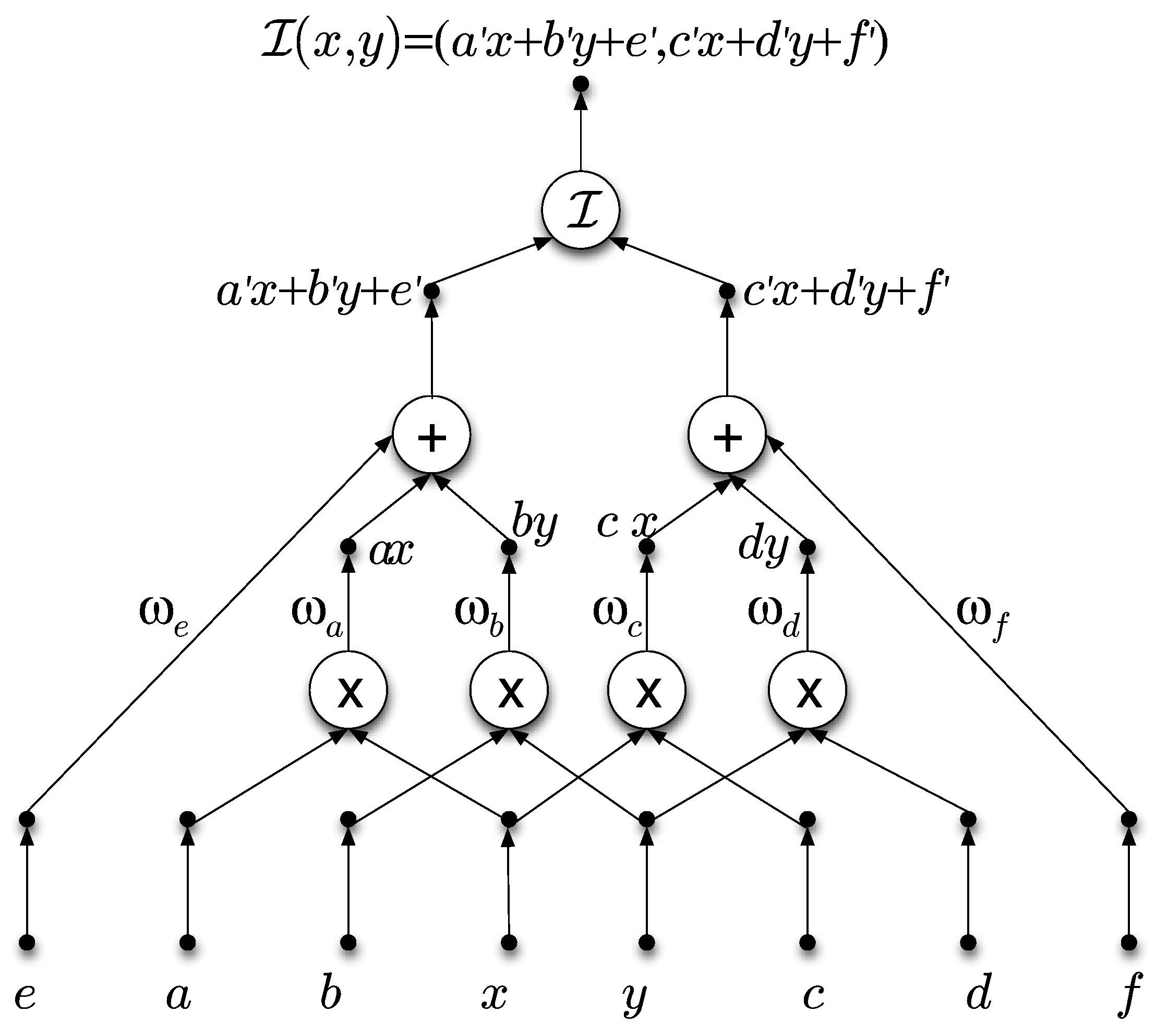
  • Layers of neurons. Similar to ANNs, neurons are represented by circles with the name of the corresponding neural function inside. For example, in Figure 1, we have two intermediate layers comprised of four and two neurons, respectively. The neural functions in the first layer and the second layer correspond to the × and the + operators, respectively.
  • Layers of storing units. This is a new component with respect to the traditional ANNs. The storing units are not neurons, and they do not process information; their task is to store intermediate information. They are represented graphically by small circles in black. The storing units are optional and generally used to allow connections of more than one neuron output to the same unit. In Figure 1, and moving upwards, we can see a first layer of eight input units storing the input information, a second layer of four storing units containing the products of two inputs, a third layer of two storing units containing the transformations of the initial variable x and y under the action of the affine contractive function in Equation (5), and a fourth (output) layer combining both outputs into a single 2D vector.
  • A set of directed links. Similar to ANNs, they are used to connect the input or intermediate layers to its adjacent layer of neurons. These connections are graphically represented by arrows to show the bottom-up flow direction from the input layer to the output layer.
  • A set of weights. Similar to ANNs, the output of the neurons can also be modulated by scalar weights. In Figure 1, there are six scalar weights corresponding to the parameters of Equation (5). These weights modify the initial parameters a , b , c , d , e , f into new values a , b , c , d , e , f . The weights are not fixed but change dynamically by reinforcement, learning along the iterations during the learning process.
To summarize, the functional networks are more general and exhibit a higher flexibility than the ANNs, which can be advantageously applied to solve more complex problems. However, it should also be remarked that the learning process is more difficult with functional networks than with ANNs; because the weights are no longer numbers but functions, the learning process requires the solving of a set of functional equations, which is harder than solving the system of equations that typically arise in ANNs [37].

4. The Problem

As discussed in Section 2.6, the collage theorem implies that any digital image I in R 2 can be graphically approximated through an IFS. More precisely, it is possible to find an IFS { F 1 , F 2 , , F N } such that its attractor H ( B ) can approximate I according to a similarity error function Ψ that computes the distance between both compact sets, I and H ( B ) . Furthermore, according to the discussion in Section 2.4, such an attractor can be obtained from any initial non-empty compact set B .
Unfortunately, the collage theorem does not provide any indication about how to obtain the IFS; it just states that such an IFS exists. Thus, while it is very easy to graphically obtain the attractor with a given IFS { F 1 , F 2 , , F N } , the inverse problem (i.e., obtaining the associated IFS with a given graphical representation of an attractor) has been revealed to be extremely difficult. In fact, the literature still lacks a reliable method of determining the IFS that approximates a given image accurately. In this paper, we address this inverse problem through an automatic procedure based on functional networks, as explained in Section 5. Note that solving this inverse problem implies determining the number of contractive maps of the IFS along with their parameters; in other words, determining the IFS code, which is given by the set { ξ i j k , τ i k } i , j = 1 , 2 ; k = 1 , , N . This problem, sometimes referred to as the IFS encoding, can be formulated as a minimization problem given by the following equation:
m i n i m i z e { ξ i j k , τ i k } i , j = 1 , 2 ; k = 1 , , N Ψ I , H ( B )
for some similarity error function Ψ .
This problem in Equation (6) is a very difficult one for several reasons. On the one hand, the problem is continuous and high-dimensional since all variables of the problem are real-valued, and complex images can require a large number of contractive maps to be accurately reconstructed. It is also constrained because the affine maps F k of the IFS have to be contractive. On the other hand, the problem is multimodal, which means that there can be several global or local optima of the similarity error function. As a result, this problem has proven to be unsolvable with the application of traditional mathematical optimization techniques. Although many alternative techniques have been described in the literature, as discussed in Section 1.2, the problem remains unsolved to a large extent. In this context, a new method based on functional networks is proposed in this paper. This will be discussed in next section.

5. The Method

5.1. Overview of the Method

The method proposed in this paper relies on functional networks to solve the optimization problem given by Equation (6). The input of the network is a binary (black and white) image of p × q pixels, where the actual pixels of the image appear in black. The image is mathematically described as a matrix M of size p × q , where each entry m i , j takes a value of 1 if the corresponding pixel ( i , j ) of the image is colored in black, and a value of 0 if otherwise. The output of the method is the IFS code of an IFS { F 1 , F 2 , , F N } of N contractive maps, where N is a parameter freely chosen by the user. A functional network with the structure shown in Figure 1 is used for each contractive map of the IFS. The resulting N functional networks are combined in a general network with the structure shown in Figure 2. As shown in that figure, the method takes the different pixels ( x , y ) of the given image as the input of N functional networks. Each functional network F N j is used to compute the IFS code of the corresponding contractive map F j . The input of the functional network is given by the pixel ( x , y ) and the values of the parameters of the IFS code of F j , assumed to be randomly initialized with uniform distribution but subjected to the constraints of contractivity (if the random values do not satisfy such constraints, new random values are taken). The learning process proceeds iteratively: at each generation, the network is presented with all the pixels of the input image. Then, based on their previous values, each functional network computes new values for the IFS code. Such values are stored in an output matrix of the IFS code of the image, which is used to generate the reconstructed image through the procedure described in Section 2.4 and Section 2.5. Next, the network computes the similarity error between the input image and the reconstructed image. This iterative process can be repeated for a given number of iterations, denoted onwards as M, or until the similarity error is below a prescribed threshold.

5.2. Similarity Error Function

The optimization problem in Equation (6) depends on a similarity error function computing the distance between the original and the reconstructed images. A natural choice would be the Hausdorff distance, defined in Equation (2), but it is highly demanding computationally and hence inefficient for large images. Fortunately, several alternative functions can be chosen for this purpose.
Our function is based on the Hamming distance, a popular choice to measure distances between binary strings. If the original and reconstructed images, denoted onwards as O and R , are represented mathematically by two matrices of binary values 0 and 1 and of equal dimensions p × q , the Hamming similarity error function S H between O and R can be obtained as follows:
S H ( O , R ) = 1 p × q x = 1 p y = 1 q O ( x , y ) R ( x , y )
which is a function taking values on the interval [ 0 , 1 ] , where the value 0 means that both images are identical.

6. Computational Procedure and Results

6.1. Computational Procedure

The method described in the previous section has been applied to some examples of binary fractal images. In this section, we describe one of such examples in detail. The example is shown in Figure 3, where the fractal is displayed as a binary image (i.e., in black and white) on the left and as a colored image on the right, where a different color is selected for each contractive map. We remark, however, that the color is used only for illustrative purposes and does not play any role in the method. The input image used in our method is the binary image on the left.
We apply our method as explained in Section 5. The input of the method is the fractal image in Figure 3 (left), represented numerically by a binary matrix of size 600 × 600 . The number of active (black) pixels in the image is 65,532. The network in Figure 2 is applied iteratively for M = 1200 iterations, following the procedure described in Section 5.1. In our trials, this number of iterations was enough to ensure the convergence of the process in our experiments.

6.2. Graphical Results

Figure 4, Figure 5 and Figure 6 show the evolution of the reconstructed image from the initial to the final iteration, every 20 iterations. The figures are shown here to illustrate how the functional network-based method actually works. As explained above, the method is initialized with random values for the IFS parameters, leading to an image that is graphically very different from the target image of Figure 3 (left). During the learning process, the network updates the values of the IFS parameters, leading to images that slowly converge towards the target. The reconstructed image corresponds to the last image in Figure 6.
A simple visual comparison with Figure 3 (left) shows the close resemblance between the original and the reconstructed images. From the graphical results, we can conclude that the method performs quite well as it is able to recover the general shape of the image with high visual accuracy. This result is remarkable since the process starts with a random IFS code. Furthermore, the target image exhibits a complicated and irregular shape, which makes it hard to figure out the possible values of the IFS parameters. However, even in this case, not only the general shape but also all major features of the image are faithfully recovered.
Nevertheless, we noticed that the original and the reconstructed images, albeit quite similar visually, are not identical. Since it is hard to check this fact by a simple visual comparison of the original and the reconstructed images, we also compute the intersection and the union operators of both images every 20 iterations. The corresponding graphical outputs are shown in Figure 7, Figure 8 and Figure 9 for the intersection operator, and in Figure 10, Figure 11 and Figure 12 for the union operator. We use reverse colors in all these figures for a better visualization of their main features.
The intersection and union operators are very useful for quantifying the differences between the original and the reconstructed images over the iterations as they account for the common points and the active areas of the image, respectively. Ideally, the final images for both operators should be identical to the original image for perfect matching.
Clearly, this does not happen here. Although the original and the reconstructed images are quite similar, there are still some visual differences. In other words, there is no perfect match with this approach, which means that our method still has room for further improvement.

6.3. Numerical Results

The graphical results of the method are confirmed by the numerical data. Table 1 shows the number of iterations (denoted as iter) of the method (with a step size of 20), the number of pixels with a different binary value for the original image I and the reconstructed image R (denoted as I R ), and the similarity between both images. This similarity is obtained as 1 S H , where S H is the similarity error computed according to Equation (7). Note that a similarity of 1 means a perfect match between both images.
As the reader can see, the method slowly improves over the iterations. The number of different points between the images evolves—from a very large number of 124,490 pixels at the initial iteration to 57,551 points at the final iteration—leading to a reduction rate of about 216% for the number of different pixels. The process converges to a final value of the Hamming similarity, at 1 S H = 0.840136 for iteration 1200. This value of similarity obtained with our method is very remarkable. To the best of our knowledge, no other neural network-based method reported in the literature so far has achieved this level of matching for a fractal image using only the initial binary image as the input. At the same time, our results mean that there is a mismatch of about 16 % between the images. This provides an indication that the method performs very well but could probably be further improved.

6.4. Comparison with Other Approaches

As remarked in Section 1.2, a few methods have been applied to the IFS inverse problem with modest success. In this comparative work, we consider four of the most popular alternative methods: an artificial neural network [39], simulated annealing [44], genetic algorithms [45], and the firefly algorithm [46]. These methods have been chosen to represent different families of methods. The artificial neural networks are one of the most popular and widely used approaches in artificial intelligence; simulated annealing is one the most popular single-particle methods; genetic algorithms are the best known evolutionary methods; and the firefly algorithm is a recent yet popular population-based nature-inspired swarm intelligence method. For the neural network, we consider a multilayer perceptron (MLP), which is well-known to be a universal function approximator. In our comparative work, we consider an MLP with 12 N neurons, with N being the number of contractive maps of the IFS. To make the comparison as fair as possible, for the genetic algorithms and the firefly algorithm, we consider a population of 6 N individuals (as many as the number of neurons in our method). We also consider a total of 1200 iterations (as many as the number of iterations in our method) for the MLP, genetic algorithms, and firefly algorithm methods. On the other hand, we consider a total of 6 N × 1200 iterations for the simulated annealing to balance the drawback of using only a single particle and use a number of evaluations of the fitness function, similar to the other methods.
Table 2 shows the comparative results between the similarity rate values of the four alternative methods and the method proposed in this paper. The results show that our proposed method outperforms the other methods used in this comparison. This is a clear evidence of the advantages of the presented method in addressing the IFS inverse problem. We remark, however, that the method is not yet optimal, and more accurate methods should be expected to appear in the future.

6.5. Computational Issues and CPU Times

Regarding the computational times of our approach, they depend on the complexity of the input image, the number of contractive maps, the number of iterations, the error threshold (if any), and other factors. As a consequence, it is difficult to determine the CPU time of a given example in advance. However, our trials on several examples show that a typical execution can take from a few minutes to 2–3 h (including the learning phase), depending on the factors indicated above. These CPU times are competitive with the reported times of other alternative methods, although a direct comparison is difficult in some cases as some of the papers were published some time ago. In any case, we noticed that the method is time-consuming and hence unsuitable for real-time applications or practical settings requiring a very fast result. This is one of the limitations of this work; our focus in this paper is on accuracy rather than on the computational speed.
All simulations in this work were performed using a computer code implemented by the authors on the popular scientific program Mathematica, running on a personal computer with a 3.7 GHz Intel Core i7 processor and 8 GB of RAM.

6.6. Computational Complexity

Regarding the computational complexity of the method, the execution of each functional network at each iteration requires 4 sums and 10 products, and hence shows linear complexity. The computation is performed for N functional networks and for the p × q pixels of the image, so the complexity becomes O ( N ( p × q ) ) . Considering a number of M iterations, it yields a total of O ( M . N ( p × q ) ) , excluding rendering. This improves the computational complexity of the multilayer perceptron (MLP) neural network (a well-known universal function approximator), which becomes O ( n 2 . M . ( p × q ) ) for this problem and where n is the number of neurons. For a more complete comparison, we also consider state-of-the-art evolutionary methods such as genetic algorithms or particle swarm optimization. The computational complexity of the genetic algorithms is O ( M ( N . S + N . S + N ) ) , where M is the number of generations, N the population size, and S the size of each chromosome, which in this case yields a total of O ( M ( 2 N ( p × q ) + N ) ) , leading to longer computational time than that required by our method. The same happens with particle swarm optimization, with a computational complexity of O ( ( 2 M . N + 5 M + 3 ) ( p × q ) + ( M 1 ) N + 6 ) for the problem in this paper. The results show that while the order of the computational complexity is comparable for genetic algorithms, particle swarm optimization, and our method (order O ( M . N ( p × q ) ) for the three methods), the total number of operations is lower for our method.

7. Conclusions and Future Work

In this work, a new method for solving the problem of image reconstruction of binary images with IFS is proposed. The method is based on functional networks, a kind of artificial network that extends the classical neural networks in several ways. In this paper, we use an artificial network that is comprised of several functional networks. Each functional network computes the IFS parameters of one of the contractive affine functions as part of the IFS. A challenging example of a binary fractal image with a complex shape is used to check the performance of the proposed method. The graphical results show that the method performs very well as the general visual structure and all major graphical details are reconstructed with high accuracy. The numerical results confirm the good visual results but also shows that the method still provides sub-optimal results that can probably be further improved.
Several future lines of research can be proposed based on this work. A major open question is how to improve the accuracy of the reconstruction method. The combination of this technique with local search methods might improve the search ability of the optimal values, especially at later stages of the method, when the values are in the neighborhood of the optima. Another challenge is the reduction of the computation time of the method. In our implementation, we did not apply any strategy for parallelization. However, we remark that the N functional networks can work in parallel, as they actually compute values of different contractive maps, which are then combined to form the IFS. This represents a promising avenue for drastically reducing CPU times. Finally, the functional networks here work as building blocks of a more general artificial network. Following this idea, the functional networks might also be embedded into deep learning methodologies, where several layers of functional networks could be used to improve the learning capabilities of the network. Finally, the extension of this method to non-binary images is also part of our plans for future work in the field.

Author Contributions

Conceptualization, A.G., A.I., I.F., I.F.J., V.G.-J., C.M., and C.O.; methodology, A.G., A.I., I.F.J., V.G.-J., C.M., and C.O.; software, A.G., I.F.J., V.G.-J., and C.M.; validation, A.G., I.F., C.M., and C.O.; formal analysis, A.I., I.F., V.G.-J., and C.O.; writing—original draft preparation, A.I., I.F.J., V.G.-J., and C.O.; writing—review and editing, A.G., A.I., I.F., I.F.J., and C.O.; supervision, A.G., A.I., I.F., and C.O.; project administration, A.G., A.I., I.F., I.F.J., and C.O.; funding acquisition, A.G., A.I., I.F., I.F.J., and C.O. All authors have read and agreed to the published version of the manuscript.

Funding

This research was funded by the project PDE-GIR of the European Union Horizon 2020 Research and Innovation Programme under the Marie Sklodowska- Curie Grant Agreement No. 778035, and by the project TIN2017-89275-R, funded by the State Research Agency of the Spanish Ministry of Science and Innovation, MCIN/AEI/10.13039/501100011033/FEDER “Una manera de hacer Europa”. Iztok Fister and Iztok Fister, Jr. are also grateful for the financial support from the Slovenian Research Agency (Research Core Funding No. P2-0042 and No. P2-0057, respectively).

Institutional Review Board Statement

Not applicable.

Informed Consent Statement

Not applicable.

Data Availability Statement

Not applicable.

Conflicts of Interest

The authors declare no conflict of interest. The funders had no role in the design of the study; in the collection, analyses, or interpretation of data; in the writing of the manuscript, or in the decision to publish the results.

References

  1. Barnsley, M.F. Fractals Everywhere, 2nd ed.; Academic Press: San Diego, CA, USA, 1993. [Google Scholar]
  2. Barnsley, M.F.; Hurd, L.P. Fractal Image Compression; AK Peters/CRC Press: Boca Raton, FL, USA, 1993. [Google Scholar]
  3. Falconer, K. Fractal Geometry: Mathematical Foundations and Applications, 2nd ed.; John Wiley & Sons: Chichester, UK, 2003. [Google Scholar]
  4. Fisher, Y. (Ed.) Fractal Image Compression: Theory and Applications; Springer: Berlin, Germany, 1995. [Google Scholar]
  5. Peitgen, H.O.; Jurgens, H.; Saupe, D. Chaos and Fractals. New Frontiers of Science; Springer: New York, NY, USA, 1993. [Google Scholar]
  6. Gutiérrez, J.M.; Iglesias, A.; Rodríguez, M.A.; Rodríguez, V.J. Generating and rendering fractal images. Math. J. 1997, 7, 6–13. [Google Scholar]
  7. Barnsley, M.F.; Demko, S. Iterated function systems and the global construction of fractals. Proc. R. Soc. Lond. 1985, A399, 243–275. [Google Scholar]
  8. Barnsley, M.F.; Ervin, V.; Hardin, D.; Lancaster, J. Solution of an inverse problem for fractal and other sets. Proc. Natl. Acad. Sci. USA 1986, 83, 1975–1977. [Google Scholar] [CrossRef] [PubMed] [Green Version]
  9. Hutchinson, J.E. Fractals and self similarity. Indiana Univ. Math. J. 1981, 30, 713–747. [Google Scholar] [CrossRef]
  10. Gonzalez, R.C.; Woods, R.E. Digital Image Process, 4th ed.; Pearson: London, UK, 2018. [Google Scholar]
  11. Barnsley, M.F.; Sloan, A.D. A better way to compress images. BYTE Magazine, January 1988. [Google Scholar]
  12. Jacquin, A.E. Image coding based on a fractal theory of iterated contractive image transformations. IEEE Trans. Image Process. 1992, 1, 18–30. [Google Scholar] [CrossRef] [Green Version]
  13. Berkner, K. A wavelet-based solution to the inverse problem for fractal interpolation functions. In Fractals in Engineering’97; Véhel, L., Lutton, E., Tricot, C., Eds.; Springer: London, UK, 1997. [Google Scholar]
  14. Wadstromer, N. An approach to the inverse IFS problem using the Kantorovich metric. Fractals 1997, 5, 89–99. [Google Scholar] [CrossRef]
  15. Abenda, S.; Demko, S.; Turchetti, G. Local moments and inverse problem for fractal measures. Inv. Probl. 1992, 8, 739–750. [Google Scholar] [CrossRef]
  16. Forte, B.; Vyrscay, E.R. Solving the inverse problem for measures using iterated function systems: A new approach. Adv. Appl. Prob. 1995, 27, 800–820. [Google Scholar] [CrossRef]
  17. Vyrscay, E.R. Moment and collage methods for the inverse problem of fractal construction with iterated function systems. In Fractals in the Fundamental and Applied Sciences; Peitgen, H.O., Henriques, J.M., Penedo, L.F., Eds.; Elsevier: Amsterdam, The Netherlands, 1991. [Google Scholar]
  18. Saupe, D.; Hamzaoui, R. A review of the fractal image compression literature. Comput. Graph. 1994, 28, 268–276. [Google Scholar] [CrossRef]
  19. Gutiérrez, J.M.; Cofino, A.S.; Ivanissevich, M.L. An hybrid evolutive-genetic strategy for the inverse fractal problem of IFS Models. Proceedings of the International 7th Ibero-American Conference on AI, IBERAMIA 2000. In Advances in Artificial Intelligence; Springer: Berlin/Heidelberg, Germany, 2000; Volume 1952, pp. 467–476. [Google Scholar]
  20. Lutton, E.; Véhel, J.L.; Cretin, G.; Glevarec, P.; Roll, C. Mixed IFS: Resolution of the Inverse Problem Using Genetic Programming; INRIA Rapport 2631; INRIA: Rocquencourt, France, 1995. [Google Scholar]
  21. Wu, M.S.; Teng, W.C.; Jeng, J.H.; Hsieh, J.G. Spatial correlation genetic algorithm for fractal image compression. Chaos Solitons Fractals 2006, 28, 497–510. [Google Scholar] [CrossRef]
  22. Wu, M.S.; Jeng, J.H.; Hsieh, J.G. Schema genetic algorithm for fractal image compression. Eng. Appl. Artif. Intell. 2007, 20, 531–538. [Google Scholar] [CrossRef]
  23. Yuan, W.X.; Ping, L.F.; Guo, W.S. Fractal image compression based on spatial correlation and hybrid genetic algorithm. J. Vis. Commun. Image R 2009, 20, 505–510. [Google Scholar] [CrossRef]
  24. Zheng, Y.; Liu, G.R.; Niu, X.X. An improved fractal image compression approach by using iterated function system and genetic algorithm. Comput. Math. Appl. 2006, 51, 1727–1740. [Google Scholar] [CrossRef] [Green Version]
  25. Dasgupta, D.; Hernandez, G.; Niño, F. An evolutionary algorithm for fractal coding of binary images. IEEE Trans. Evol. Comput. 2000, 4, 172–181. [Google Scholar] [CrossRef] [Green Version]
  26. Gálvez, A.; Iglesias, A.; Diaz, J.A.; Fister, I.; López, J.; Fister, I., Jr. Modified OFS-RDS bat algorithm for IFS encoding of bitmap fractal binary images. Adv. Eng. Inform. 2021, 47, 101222. [Google Scholar] [CrossRef]
  27. Muruganandham, A.; Wahida, R.S.D. Adaptive fractal image compression using PSO. Procedia Comput. Sci. 2010, 1, 338–344. [Google Scholar] [CrossRef] [Green Version]
  28. Tseng, C.C.; Hsieh, J.G.; Jeng, J.H. Fractal image compression using visual-based particle swarm optimization. Image Vis. Comput. 2008, 26, 1154–1162. [Google Scholar] [CrossRef]
  29. Evans, A.K.; Turner, M.J. Specialisation of evolutionary algorithms and data structures for the IFS inverse problem. In Proceedings of the Second IMA Conference on Image Processing: Mathematical Methods, Algorithms, and Applications; Turner, M.J., Ed.; Ellis Horwood Ltd.: New York, NY, USA, 1998. [Google Scholar]
  30. Goentzel, B. Fractal image compression with the genetic algorithm. Complex. Int. 1994, 1, 111–126. [Google Scholar]
  31. Nettleton, D.J.; Garigliano, R. Evolutionary algorithms and a fractal inverse problem. Biosystems 1994, 33, 221–231. [Google Scholar] [CrossRef]
  32. Shonkwiler, R.; Mendivil, F.; Deliu, A. Genetic algorithms for the 1-D fractal inverse problem. In Proceedings of the Fourth International Conference on Genetic Algorithms; Morgan Kaufmann: Burlington, MA, USA, 1991; pp. 495–501. [Google Scholar]
  33. Wadstromer, N. An automatization of Barnsley’s algorithm for the inverse problem of iterated function systems. IEEE Trans. Image Process. 2003, 12, 1388–1397. [Google Scholar] [CrossRef]
  34. Gálvez, A.; Fister, I.; Iglesias, A. Image reconstruction of colored bitmap fractal images through bat algorithm and color-based image clustering. In 16th International Conference on Soft Computing Models in Industrial and Environmental Applications, SOCO 2021, Advances in Intelligent Systems and Computing; Springer: Cham, Switzerland, 2021; Volume 1401, pp. 222–232. [Google Scholar]
  35. Gálvez, A.; Fister, I.; Deb, S.; Fister, I., Jr.; Iglesias, A. Cuckoo search algorithm and K-means for IFS reconstruction of fractal colored images. In Proceedings of the 8th International Conference on Soft Computing & Machine Intelligence, ISCMI-2021, Cario, Egypt, 26–27 November 2021; pp. 91–95. [Google Scholar]
  36. Elton, J.H. An ergodic theorem for iterated maps. Ergod. Theory Dynam. Syst. 1987, 7, 481–488. [Google Scholar] [CrossRef] [Green Version]
  37. Gutiérrez, J.M.; Iglesias, A.; Rodríguez, M.A. A multifractal analysis of IFSP invariant measures with application to fractal image generation. Fractals 1996, 4, 17–27. [Google Scholar] [CrossRef]
  38. Graf, S. Barnsley’s scheme for the fractal encoding of images. J. Complex. 1992, 8, 72–78. [Google Scholar] [CrossRef] [Green Version]
  39. Haykin, S. Neural Networks: A Comprehensive Foundation, 2nd ed.; Prentice Hall: Hoboken, NJ, USA, 1998. [Google Scholar]
  40. Castillo, E. Functional networks. Neural Process. Lett. 1998, 7, 151–159. [Google Scholar] [CrossRef]
  41. Castillo, E.; Iglesias, A.; Ruiz-Cobo, R. Functional Equations in Applied Sciences; Elsevier: Amsterdam, The Netherlands, 2005. [Google Scholar]
  42. Gálvez, A.; Iglesias, A.; Cobo, A.; Puig-Pey, J.; Espinola, J. Bézier curve and surface fitting of 3D point clouds through genetic algorithms, functional networks and least-squares approximation. Lect. Notes Comput. Sci. 2007, 4706, 680–693. [Google Scholar]
  43. Iglesias, A.; Gálvez, A. Hybrid functional-neural approach for surface reconstruction. Math. Probl. Eng. 2014, 2014, 13p. [Google Scholar] [CrossRef]
  44. Kirkpatrick, S.; Gelatt, C.D., Jr.; Vecchi, M.P. Optimization by simulated annealing. Science 1983, 220, 671–680. [Google Scholar] [CrossRef]
  45. Holland, J.H. Adaptation in Natural and Artificial Systems; The University of Michigan Press: Ann Arbor, MI, USA, 1975. [Google Scholar]
  46. Yang, X.S. Firefly algorithms for multimodal optimization. Lect. Notes Comput. Sci. 2009, 5792, 169–178. [Google Scholar]
Figure 1. Functional network of the contractive affine map in Equation (5).
Mathematics 10 01107 g001
Figure 2. General scheme of the network computing the IFS code of the input image.
Mathematics 10 01107 g002
Figure 3. Fractal image used in this paper: (left) in black and white; (right) in different colors for each contractive map.
Mathematics 10 01107 g003
Figure 4. (leftright, topbottom): Evolution of the reconstructed image for 0–380 iterations (step size, 20 iterations).
Mathematics 10 01107 g004
Figure 5. (leftright, topbottom): Evolution of the reconstructed image for 400–780 iterations (step size, 20 iterations).
Mathematics 10 01107 g005
Figure 6. (leftright, topbottom): Evolution of the reconstructed image for 800–1180 iterations (step size, 20 iterations).
Mathematics 10 01107 g006
Figure 7. (leftright, topbottom): Evolution of the intersection between the original and the reconstructed images for 0–380 iterations (step size, 20 iterations).
Mathematics 10 01107 g007
Figure 8. (leftright, topbottom): Evolution of the intersection between the original and the reconstructed images for 400–780 iterations (step size, 20 iterations).
Mathematics 10 01107 g008
Figure 9. (leftright, topbottom): Evolution of the intersection between the original and the reconstructed images for 800–1180 iterations (step size, 20 iterations).
Mathematics 10 01107 g009
Figure 10. (leftright, topbottom): Evolution of the union between the original and the reconstructed images for 0–380 iterations (step size, 20 iterations).
Mathematics 10 01107 g010
Figure 11. (leftright, topbottom): Evolution of the union between the original and the reconstructed images for 400–780 iterations (step size, 20 iterations).
Mathematics 10 01107 g011
Figure 12. (leftright, topbottom): Evolution of the union between the original and the reconstructed images for 800–1180 iterations (step size, 20 iterations).
Mathematics 10 01107 g012
Table 1. Evolution over the generations (iter) of the number of different pixels between the original image and the reconstructed images ( I R ) and the similarity rate ( 1 S H ).
iter I R 1 S H iter I R 1 S H iter I R   1 S H
0124,4900.65419440073,8620.79482880076,1660.788108
2098,9490.72514242073,4620.79593982075,2930.790853
4091,2950.74640344077,3950.78501484073,4710.795914
6087,7600.75622246075,0330.79157586071,3920.801689
8085,9950.76112548074,3330.79351988070,1910.805025
10082,0180.77217250074,0900.79419490069,3860.807261
12079,7340.77851752073,8090.79497592069,7480.806256
14079,3780.77950654073,6750.79534794068,7450.809042
16078,5530.78179756073,2550.79651496067,9430.811269
18078,1140.78023958072,1050.79256998067,7480.811811
20077,5820.78449460072,6270.799708100066,8500.814306
22075,4100.79052862072,5990.798258102065,9690.816753
24074,6930.79251964073,4390.798336104065,2950.818625
26073,9540.79457266073,5580.796003106065,8690.817031
28073,6260.79548368072,2190.795672108064,7760.820067
30073,5510.79569270072,8410.799392110063,0460.824872
32072,1720.79952272072,2140.797664112062,8970.825286
34073,9990.79444774074,2510.799406114061,0360.830456
36074,6670.79259276077,7140.793747116059,8560.833733
38074,2560.79373378076,2810.784128118057,5510.840136
Table 2. Comparative results between our method and four alternative approaches in the literature (the best result is in bold).
MethodSimilarity Rate
Multilayer perceptron [39]0.3287
Simulated annealing [44]0.2516
Genetic algorithms [45]0.6783
Firefly algorithm [46]0.4423
The proposed method0.8401
Publisher’s Note: MDPI stays neutral with regard to jurisdictional claims in published maps and institutional affiliations.

