Abstract
Osteosarcoma is a primary malignant tumor. It is difficult to cure and expensive to treat. Generally, diagnosis is made by analyzing MRI images of patients. In the process of clinical diagnosis, the mainstream method is the still time-consuming and laborious manual screening. Modern computer image segmentation technology can realize the automatic processing of the original image of osteosarcoma and assist doctors in diagnosis. However, to achieve a better effect of segmentation, the complexity of the model is relatively high, and the hardware conditions in developing countries are limited, so it is difficult to use it directly. Based on this situation, we propose an osteosarcoma aided segmentation method based on a guided aggregated bilateral network (OSGABN), which improves the segmentation accuracy of the model and greatly reduces the parameter scale, effectively alleviating the above problems. The fast bilateral segmentation network (FaBiNet) is used to segment images. It is a high-precision model with a detail branch that captures low-level information and a lightweight semantic branch that captures high-level semantic context. We used more than 80,000 osteosarcoma MRI images from three hospitals in China for detection, and the results showed that our model can achieve an accuracy of around 0.95 and a params of 2.33 M.
1. Introduction
Osteosarcoma is an aggressive bone malignancy that frequently occurs in the extremities of children and adolescents with a very poor natural prognosis [1]. The incidence of osteosarcoma is the highest among all primary malignant tumors in the world, reaching three per million, with a male-female ratio of about 1.5:1. At the same time, the survival rate of this tumor is also low. Before the 1980s, the five-year survival rate of patients with osteosarcoma was less than 20% [2,3,4]. This kind of tumor has a high degree of malignancy and is prone to metastases, even to the lungs, so its treatment is also more difficult. But early detection and treatment can improve patients’ survival and reduce the chance of amputation. In clinical diagnosis, MRI images do not cause great radiation and biological damage to the tissue during examination and are more obvious in tissue components such as tumors and blood vessels [5], so we generally use MRI images to detect osteosarcoma.
In the current detection process of osteosarcoma MRI images, patients with osteosarcoma will generate a large amount of image data, but the proportion of valuable images is very low. According to incomplete statistics, each osteosarcoma patient will generate 600–700 pictures, but only 10–20 pictures are valuable for diagnosis [6,7,8,9]. Currently, screening and preliminary processing of raw images are still done manually by doctors. This process consumes a lot of manpower and material resources. At the same time, there is no standardized definition of the diagnostic characteristics of osteosarcoma. Therefore, the identification of osteosarcoma requires doctors to have solid professional knowledge [10]. The average hospital does not have a complete auxiliary segmentation system for osteosarcoma, and it is difficult to diagnose patients efficiently, so the detection cost and difficulty of osteosarcoma are very high [11,12,13].
Osteosarcoma detection is costly and difficult. The medical system in most developing countries is not perfect, so there are great difficulties in the diagnosis, treatment and prognosis of osteosarcoma. Taking China as an example, China’s per capita medical resources are relatively low, professional talents are scarce, and medical resources are relatively tight. The expensive and sophisticated testing equipment only exists in large general hospitals. Rural people often delay what is the optimal time for treatment for economic and geographical reasons. Secondly, the regional distribution of public medical resources in China is uneven. 80% of medical resources are concentrated in developed areas with only 10% of the population. The risk of death is greatly increased due to the rapid diagnosis and treatment of osteosarcoma. These problems have brought a heavy burden to societies and families in developing countries [14]. It is essential to have an efficient and accurate assisted segmentation system for osteosarcoma.
With the emergence of medical intelligent image detection technology, the problem of low medical diagnosis efficiency of osteosarcoma in developing countries has been alleviated to a certain extent. This technology uses edge detection, template matching, deep learning and other methods to segment key targets in MRI images and extracts features from the segmented regions, thereby realizing the automatic segmentation of osteosarcoma images and assisting in judging the presence and status of osteosarcoma [15,16,17]. However, there will also be some local tissue formation on the edge of osteosarcoma, which leads to uncertain and unclear tumor boundaries. At the same time, the anatomical structure and shape of osteosarcoma images are usually complicated, and the imaging principles are also different, in addition to the presence of noise in the image, so the effect of segmentation is often unsatisfactory. In order to improve the accuracy of image segmentation and optimize the segmentation effect, researchers perform a large number of artificial feature extractions and consider the implicit features of medical images. However, the parameter size and complexity of the segmentation model will be increased accordingly, and the inference speed will be very slow. In the process of medical image processing, the inference speed of the model will affect the time of diagnosis and even the treatment of patients. In order to speed up the inference speed of the model, the principle of the current method is almost sacrificing the underlying details, which will lead to a decrease in the accuracy of the segmentation model. Therefore, it is very important to establish a segmentation model that finds a balance between speed and accuracy.
Based on the above analysis, this paper proposes an osteosarcoma aided segmentation method based on a guided aggregated bilateral network (OSGABN). In this system, we first optimize the dataset and divide the dataset into useful slices (US) and difficult slices (NS) according to availability. This method solves the overfitting caused by time scrambling and fast deep learning models. Then we preprocess the MRI image, in which we add more features to improve the median filter and generate a simple and effective noise reduction method for medical images, which can significantly reduce various noise interference. At the same time, we use curvelet transform for image enhancement to locally enhance the tumor region to further reduce unwanted noise in the input image. We then used the fast bilateral segmentation network (FaBiNet) for osteosarcoma MRI image segmentation. This network structure is efficient and effective; there is a detail branch and a semantic branch in this segmentation network, and the detail branch has wide channels and shallow layers, which can capture low-levels and generate high-resolution feature representations. The semantic branch channel is narrow but deep, and high-level semantic context can be obtained. Because of the lightweight semantic branch, it can effectively reduce the channel capacity and speed up the downsampling speed. On the basis of strong segmentation performance, the reasoning cost is reduced, and it has great advantages, such as a fast training speed and balance between speed and accuracy.
The main contributions of this study are as follows:
- (1)
- This paper uses the mean teacher model to optimize the classification of the data set, divide the data set into US and NS, and input them into the network in different orders for training, which further improves the training efficiency.
- (2)
- We use the fusion noise reduction method to preprocess the image, which improves the accuracy of model training and improves the robustness of the model.
- (3)
- This paper adopts the image segmentation model based on the fast bilateral segmentation network. While achieving high-precision segmentation, it uses an extremely lightweight model which greatly improves the speed of segmentation, so it has great significance in practical applications.
- (4)
- We used more than 80,000 samples collected by the Second Xiangya Hospital of Central South University for experimental analysis. The structure shows that our osteosarcoma segmentation method has a better segmentation effect than other methods, and the model is highly lightweight, which is convenient for training and application. This method is of great significance to the diagnosis, treatment and prognosis of osteosarcoma. Doctors can use the diagnosis results as an auxiliary basis for diagnosis and treatment, and greatly reduce the pressure of doctors and the time of diagnosis without affecting the accuracy.
2. Related Works
In the current research, the use of advanced computer technology to process medical images to complete the auxiliary diagnosis of diseases such as osteosarcoma has been called a trend. Many people are already using technologies such as artificial intelligence and image processing to achieve these goals. We will introduce some mainstream methods and related systems in the following analysis.
Mohamed Nasor and Walid Obaid [18] combined morphological operations and object technology to segment osteosarcoma MRI images utilizing K-means clustering and Chan-Vese, and achieved good segmentation results. Limei Shuai, Xin Gao, and Jiajun Wang [19] et al. proposed a novel W-net++ architecture based on two cascaded U-Nets and dense skip connections when studying the image segmentation of osteosarcoma, and introduced adaptive depth supervision, which effectively improves performance. Rui Zhang, Huang Lin [20] and others proposed an end-to-end network for osteosarcoma segmentation based on deep learning. This network named MSRN added multiple supervised output modules to guide the learning of shape features and semantic features. Harish Babu Arunachalamp [21] et al. used machine learning and deep learning models to classify osteosarcoma WSI into non-tumors, necrotic tumors, and viable area tumors. Rahad Arman Nabid [22] and others proposed a sequential recurrent convolutional neural network (RCNN) that combines convolutional neural network and bidirectional gate recurrent units in order to evaluate the grading of patients with osteosarcoma. The performance of this model is acceptable, but it has problems such as overfitting. Yu Fu [23] et al. proposed a new model based on the Siamese model, named DS-Net. It can be used to classify hematoxylin and eosin-stained histological images of osteosarcoma, which can help pathologists improve the accuracy of diagnosis and even achieve zero misclassifications.
In the field of tumor image segmentation, in addition to osteosarcoma segmentation, there are many other types of tumor image segmentation, among which the related research on brain tumor image segmentation is more in-depth, and many researchers have made achievements in it. QIAO Ying-jing, GAO Bao-Iu [24] and others studied the texture features of Tamura, and they proposed an image segmentation algorithm related to improved FCM for brain MRI based on this which was linearly weighted with gray features to form fusion features. Lei Hua, Yi Gu [25] and others found that the classical c-means algorithm is very sensitive to noise and offset field, and they adopted an improved multi-view FCM clustering algorithm (INV-FCM) which has a certain adaptive ability. In recent years, multi-level thresholding has become a widely used segmentation method in medical image analysis, but as the threshold increases, the efficiency of the algorithm will decrease. In order to solve this problem, Omid Tarkhaneh and Haifeng Shen [26] et al. proposed adaptive differential evolution (ALDE) with Levy distribution to obtain optimal thresholds at a reasonable cost. E. Sasikala, P. Kanmani [27] et al. used the fractional BAT algorithm Fuzzy C to find disbelief regions from MRI images, and realized lesion identification for MRI brain image segmentation using this hybrid algorithm.
There are many researchers who enhance the function of image segmentation by optimizing the structure of the model and carrying out appropriate improvement measures. In the research process, DM Anisuzzaman and Hosein Barzekar [28] and others fine-tuned CNN and other tools to propose the VGG19 model, which has the highest recognition rate of 96%. Haimei Chen, Xiao Zhang [29] et al. constructed a CE FS T1WI radiomic signature in developing and validating a radiomic signature for MRI, which can provide a potential tool to predict a pathological response to NAC in osteosarcoma patients. FCFDionsio and LSOliveirpa [30] et al. evaluated intra- and inter-observer reproducibility of manual segmentation of osteosarcoma in MRI, and then they compared manual versus semi-segmented methods, and found that the degree of similarity between the two segmentation methods to be very high and that using a semi-automatic method can greatly reduce the time required. Esha Baidya Kayal, Devasenathipathy Kandasamy [31] and others adjuvanted chemotherapy in osteosarcoma, and experiments proved that their SLICs+MTh method can improve cancer treatment detection, plans and overall prognosis.
In the process of segmentation and identification of osteosarcoma images, many people easily confuse osteosarcoma with Ewing sarcoma, which affects subsequent diagnosis and treatment. So many researchers have made their contributions in identifying osteosarcoma and Ewing sarcoma. In their study, Yi Dai, Ping Yin [32] et al. used radiological analysis of T2-weighted images and enhanced T1-weighted images to differentiate them and achieved good results. In their study, safak Parlak, F. Bilge Ergen [33] and others explored the ability of the apparent diffusion coefficient to differentiate between Ewing sarcoma and osteosarcoma, and obtained MW and ADC values that could be used to differentiate Ewing sarcoma from bone flesh. James R Barnett, Panagiotis Gikas [34] and others, in the study of MRI images of osteosarcoma and Ewing sarcoma, found that MRI images have high sensitivity, specificity and diagnostic accuracy in identifying skip metastases in these two tumors. Raquel Bezerra Guerra [35] et al. described early signs and symptoms of both sarcomas and identified symptoms that could be used to help differentiate the two tumors, providing subsequent researchers with valuable information and experience.
3. Methods
Osteosarcoma is a malignant tumor that occurs frequently in children and adolescents, and its prognosis is generally poor [36]. Manual screening and detection by doctors alone is inefficient, and the workload of doctors is obviously significant. Therefore, automatic image processing by computer is used in order to run the segmentation model on low-cost hardware. This paper develops an osteosarcoma aided segmentation method based on guided aggregated bilateral network-based network (OSGABN), which is used to help doctors initially identify MRI images of osteosarcoma so as to achieve the efficient and rapid identification and diagnosis of osteosarcoma. The overall design of this system is shown in Figure 1.
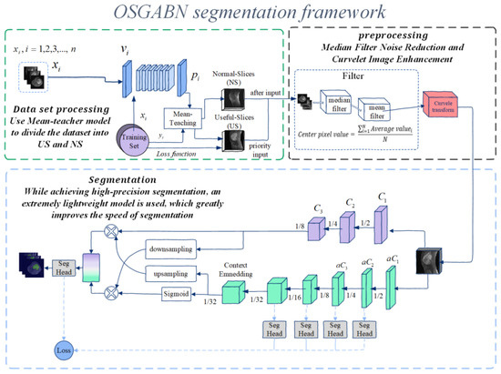
Figure 1.
Overall architecture diagram of OSNDCN.
This model is documented in two parts; the first part is the preprocessing before segmentation of osteosarcoma MRI images, and the second part is the segmentation part of the system. In the first part, the patient’s MRI image is input into the segmentation system, the data is processed and enhanced before segmentation, the data set is segmented, the noise level of the image is reduced, and then it is inputted into the segmentation network for training. The second part is the assisted segmentation of osteosarcoma MRI images using a guided aggregated bilateral network. After segmentation, it can provide a valuable reference for the doctor’s follow-up diagnosis and judgment of the degree of soft tissue invasion and play a role in auxiliary diagnosis. We list some symbols used in this paper in Table 1.

Table 1.
Symbol description.
The overall architecture of (OSNDCN) is reflected in Figure 1, and in the first part, the MRI image is divided. This part mainly includes three structures which use the mean-teacher model to divide the original data set, preprocess the data set for noise reduction and data enhancement, and divide the bilateral network.
To further improve the detection accuracy, we set the following three strategies:
- (1)
- Data set optimization. We use the mean-teacher model to first divide the dataset into useful-slices (US) and Normal-Slices (NS), and then input them to the next step of processing.
- (2)
- Preprocessing. In the denoising process, we improve the median filter by adding more features, which results in a simple and effective denoising method for osteosarcoma MRI images and significantly reduces various noise interference. At the same time, we use curvelet transform for image enhancement to locally enhance the tumor region to further reduce unwanted noise in the inputted image.
- (3)
- Guided aggregation bilateral network segmentation algorithm. In this algorithm, we deal with the low-level details and high-level semantics separately to achieve high-precision and high-efficiency real-time semantic segmentation. In addition, we design a guided aggregation layer to enhance the interconnection and fusion of two types of feature representations, with good segmentation performance.
3.1. Dataset Optimization
The amount of data in the initial dataset is large, but not every image is suitable for input into the model for training. In some MRI images, the tumor location is not clearly visible or even visible to the naked eye. These MRI images contain noise, but they can still help with model training. Using these data directly will greatly affect the training effect, so we need to classify the original data set, divide the MRI images into US and NS, first input the US into the network for training, and then input the MRI images in the NS for training, and then the newly added slice collection can be processed continuously. We use the mean-teacher semi-supervised algorithm, and the partition network population is divided into a student model and a teacher model. The network parameters of the student model are obtained by learning and gradient descent, and the loss function includes two parts: one is the supervised loss function, which is used to ensure the fitting of the labeled training data; the other is the unlabeled loss function, which is used to make sure that the predictions of the student model are as similar as possible to those of the teacher model. The network parameters of the teacher model are obtained by moving the average of the network parameters of the student model.
To accomplish this task, we set up a ResNet-7 network to partition the dataset, as shown in Figure 2. ResNet-7 is composed of six layers of residual modules and one layer of fully connected modules. The residual module uses the idea of a residual to avoid vanishing gradients. A 3 × 3 max pooling layer is set between each connected layer to reduce the size of the feature map, and the last fully connected layer performs the final classification. The parameter groups of the student model and the teacher model are . We randomly divide the original dataset into and , where has the label , and has no label. The training process of this algorithm is as follows:
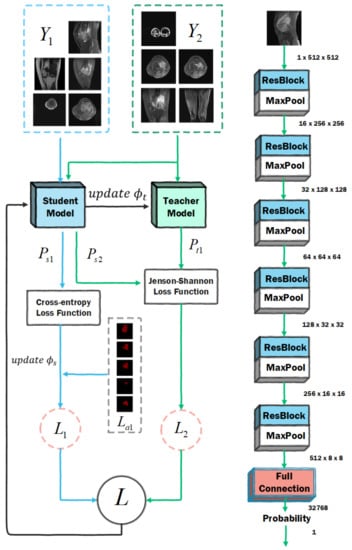
Figure 2.
Dataset optimization network architecture diagram.
- (1)
- Input and into the student model, and the output is the predicted probability ; input into the teacher model, and output the predicted probability ;
- (2)
- Calculate the loss value according to and , and the calculation equation of is:
- (3)
- Calculate the loss value and the loss equation according to and ;
- (4)
- The loss value of the student model is , the update parameter using this gradient descent is , and the teacher network updates the parameter by moving average to , and the update process is expressed by the Equation (2).
For dataset , due to the existence of labels, the loss function is a cross-entropy loss function, and the dataset has no labels, so the loss function needs to use the Kullbac-Leibler (KL) divergence relative entropy loss function; relative entropy is generally used to describe the degree of overlap between two distributions. If they overlap completely, its value is 0. If they do not overlap, its value is 1. KL is generally shown in the Equation (3):
However, the KL function will always have asymmetric problems. We hope that the prediction distributions of the teacher model and the student model are as consistent as possible, but it is impossible to judge which party has a more accurate prediction result, so we use the Jenson-Shannon (JS) algorithm to compensate for the asymmetry problem, and the calculation of can be expressed as follows:
After the above process, we successfully divided the dataset into two parts, in which US accounted for 54.6% and NS accounted for 45.4%, and then input them into the segmentation network in turn. In this way, the deep network will first learn simple samples and train a model with good performance.
3.2. Preprocessing
3.2.1. Noise Reduction Process
First, we can denoise osteosarcoma MRI images using traditional median filtering, but the median value found in existing median filtering is not always the actual value of the composite original image. This value is always the median of the sorted results of all pixels for each odd-sized rectangular subimage window in the noisy image. We use a combination of median and mean filtering to determine more precise values for each pixel in the noisy image. The principle of this method is as follows.
Firstly, we need to calculate the median, and we consider any odd-sized rectangular subimage window or mask (e.g., 3 × 3) in the osteosarcoma MRI image, which will facilitate the determination of the median of the window. It is very convenient to use odd list sizes to find the median, and the median filter goes through the magnitudes of all vectors within the mask and sorts the magnitudes, and then replaces the pixel of interest with the pixel of the median magnitude. This median is found by filtering the existing medians.
where represents the coordinate set of the rectangular sub-window, centered at the point (x, y), and the median represents the median of the window.
After completing the above work, we start to calculate the average value of each pixel. From the above introduction, we can know that the process of calculating the average value can obtain more accurate pixel values and maximize the use of domain pixels, so each pixel in the new window we calculate will have a more accurate value. This process can be described as:
After completing the above work, we can calculate the value of the center pixel. We perform arithmetic mean filtering on all the averages of the subimage windows, computing a more precise value to replace each pixel in the noisy image. The calculation method is as follows:
In Equation (7), N is the product of ROW and COLUMN of the sub-image window, that is, N = ROW × COLUMN. Through such a noise reduction process, a more accurate value of each pixel point of the noise image in the osteosarcoma MRI image is determined, so that the noise is obviously reduced, which is convenient for subsequent training.
3.2.2. Data Augmentation Process
We utilize the curvelet transform to enhance the trained images to reduce unwanted noise in osteosarcoma MRI images by enhancing the tumor region. This enhancement technique is relatively simple to implement, with high stability and short processing time. On this basis, we use curvelet transform to achieve the maximum recovery of edge and fuzzy linear features as well as curve features, which makes the boundaries of tissues such as tumor edges in MRI images clearer. In the ridgelet transform, the anisotropic scale relationship is used to realize the support interval and scale, the multi-scale ridgelet is used to decompose the osteosarcoma edge or curve into blocks and sub-blocks, and these sub-blocks are roughly regarded as straight lines, so as to be used for the realization of ridge wave analysis, and its mathematical description is as follows:
In the above formula, the region represents the multi-level filter, ∆ represents the subband information, and T represents the detected target, which is the tumor in the osteosarcoma MRI image. These smooth windows are represented by binary squares, represented as , , which will be initialized according to the image size, and the mathematical relationship is shown in Equation (9).
Then, the resulting squares are re-normalized and returned to the unit scale, and then the renormalization operator is performed. The mathematical expression of this process is:
In this way, the two dyadic sub-bands are integrated before the ridgelet transform is implemented, and the ridgelet transform is performed after the renormalization step, as shown in Equation (12).
After the above noise reduction process, the tumor boundary in the osteosarcoma MRI image can be made clearer, the influence of image noise can be reduced, and the training effect can be further improved.
3.3. Detailed Design of Bilateral Networks
Our guided aggregation bilateral network osteosarcoma image segmentation model mainly consists of two parts, a detail branch and a semantic branch. They are finally merged by an aggregation layer, and our network concept is very general. Different convolutional models can implement it. The specific design mainly includes three key contents:
- (1)
- The channel capacity of the detail branch used to process the underlying details of the osteosarcoma image is high and shallow, and the receptive field for spatial details is relatively small. The feature representation of this branch has a large spatial size and a wide channel, so it is best not to use residual connections, otherwise, it may increase the cost and reduce the speed.
- (2)
- The semantic branch is used to capture the high-level semantics in osteosarcoma MRI images, and its channel capacity is small, the level is relatively deep, and the receptive field for categorical semantics is relatively large. This branch has a lower channel capacity than the detail branch because spatial details can be provided by the detail branch. Compared to the channel with ω (ω < 1) detail branches in our experiments, such branches are lightweight.
- (3)
- The features of the above two branches are complementary, and one of them does not know the information of the other, so we design an aggregation layer to combine these two types of feature representations. Because of the fast downsampling strategy, the spatial dimension of the output of the semantic branch is smaller than that of the detail branch. Therefore, we need to upsample the output feature map of the semantic branch to match the output of the detail branch.
3.3.1. Detailed Design of Detail Branches
The detail branch is mainly responsible for processing the spatial details of osteosarcoma MRI images, which belong to low-level information, so this branch requires rich channel capacity to encode rich spatial information. At the same time, the detail branch is only concerned with the low-level details, so we will design a shallow structure for this branch. The instantiation of the detail branch consists of three stages, and each layer is a convolutional layer, followed by batch normalization and activation functions, the stride s = 2 of the first layer of each stage, and the layers in the same stage have the same number of filters and output feature map size. In this case, the output feature map extracted by this branch is one-eighth of the original inputted osteosarcoma MRI image. The channel capacity of the minutiae branch is large, which enables the minutiae branch to encode rich spatial details. However, due to the large channel capacity, high spatial dimension, and residual structure of this branch, the memory access cost is also increased accordingly. In order to alleviate this problem, this branch mainly follows the stacking idea of the VGG network.
3.3.2. Detailed Design of Semantic Branches
Considering the large receptive field and higher computational efficiency, after referring to the characteristics of other lightweight MRI image segmentation models, we design a semantic branch. The semantic branch model adopts a fast downsampling strategy to improve the feature representation level, rapidly expands the acceptable field for MRI image segmentation, and the lesion area can be determined quickly. High-level semantics require large receptive fields, so the semantic branch adopts methods such as global average pooling, embedding global contextual responses, etc. It mainly includes the stem block structure. We use stem as the first stage of the semantic branch. This process uses two different downsampling methods to reduce the feature representation and then concatenates the output features of the two branches as the output. It has low computational cost and effective feature expression ability, and its design structure is shown in Figure 3.
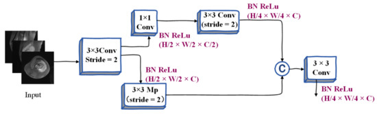
Figure 3.
Illustration of Stem Block.
Context Embedding Block. As described above, the semantic branch requires large receptive fields to capture high-level semantics, so we design the context embedding block, which uses global average pooling and residual connection methods to efficiently embed global context information. The schematic diagram of its architecture is shown in Figure 4, where Conv represents convolution operation, BN represents batch normalization, ReLu represents relu activation function, Mp refers to max pooling, and Gp refers to global average pooling. C represents the connection, 1 × 1 and 3 × 3 represent the size of the nucleus, and H × W × C represents the shape of the tensor during the segmentation of the osteosarcoma MRI image. The three parameters represent Height, Weight, and Channel, respectively.
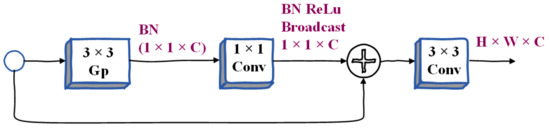
Figure 4.
Illustration of Context Embedding Block.
Gather-and-Expansion Layer. Taking advantage of deep convolutional networks, we propose a gather-expansion layer, as shown in Figure 5. The collection-expansion layer includes the following:
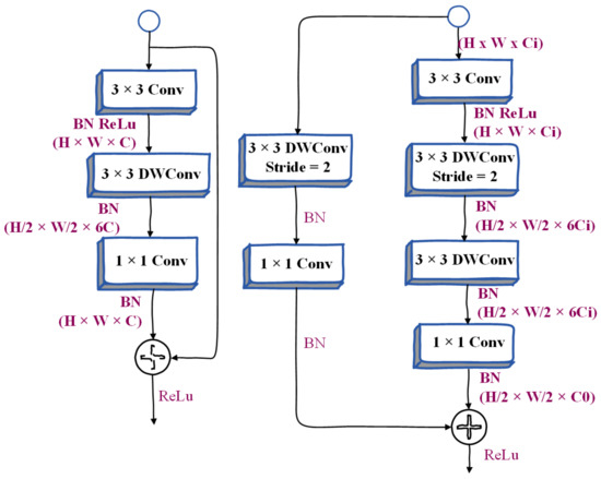
Figure 5.
Illustration of Inverted Bottleneck and Gather-and-Expansion Layer.
- (1)
- 3 × 3 convolution. Feature responses can be efficiently aggregated and scaled to higher dimensional spaces.
- (2)
- A 3 × 3 depthwise convolution can be performed independently on each output channel of the expansion layer.
- (3)
- The 1 × 1 network can be used as a projection layer to project the output of the depth-wise convolution to the space with low channel capacity. When stride = 2, we will use two 3 × 3 depth convolutions to further expand the receptive field, and a 3 × 3 separable convolution is used as a shortcut. Many people use a 5 × 5 separable convolution to expand the receptive field. Under certain conditions, its FLOPS will be better than two. There are fewer 3 × 3 separable convolutions. But in this layer, we use two 3 × 3 depthwise convolutions instead of 5 × 5 depthwise convolutions. Because this structure has fewer FLOPS and the same receptive field in our model, the model becomes more lightweight.
Compared with the inverted bottleneck in MobileNetv2, the gather-and-expansion layer has one more 3 × 3 convolutions, but the computational cost and memory access cost of this layer is relatively low. This is because the 3 × 3 convolution has been specially optimized in the CUDNN library, and with this layer, the feature expression ability of the GE layer is significantly better than the inverted bottleneck.
3.3.3. Bilateral Guided Aggregation
In order to merge the feature responses of the above two branches, researchers will adopt many methods, including a summation of elements, connection, etc. However, the outputs of the two branches have different levels of feature representation. Therefore, using a simple combination method will ignore the diversity of the two kinds of information, which will make the performance worse and the optimization difficulty will become higher. Based on our observations and experiments, we finally propose a bilateral guided aggregation layer, which uses this novel hierarchical structure to fuse the complementary information of the two branches above, as shown in Figure 6. This layer utilizes the context information of the semantic branch to guide the feature response of the detail branch. With different scale guidance, we capture different scale feature representations to inherently encode multi-scale information, while compared with the simple combination method, this bootstrapping method can make the communication between the two branches more efficient. In Figure 6, Conv is the convolution operation, DW-Conv refers to the convolution in the depth direction, aPooling refers to average pooling, BN refers to batch normalization, US refers to bilinear interpolation, and Sig refers to the sigmoid activation function. Sum refers to summation, 1 × 1, 3 × 3 represents the size of the kernel, H × W × C represents the shape of the tensor, and the three parameters represent Height, Weight, and Channel, respectively.
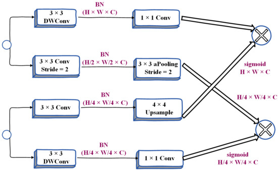
Figure 6.
Detailed design of Bilateral Guided Aggregation Layer.
3.3.4. Booster Training Strategy
After performing the main work of segmentation, we have initially separated the osteosarcoma features from the whole image. To further improve the segmentation accuracy, we propose a booster training strategy. It is a booster similar to a rocket launcher, boosting feature representations during the training phase and discarding them during the inference phase. Therefore, the computational complexity brought by it in the inference stage is very small, and we can insert auxiliary segmentation heads into different positions of the semantic segmentation model to achieve different effects. We can also adjust the computational complexity of the auxiliary split head and the main split head by controlling the channel size ct.
The above is the basic structure of our OSNDCN. Before segmentation, we performed dataset optimization and denoising operations on the original MRI osteosarcoma images. The influence of noise is reduced and the segmentation effect of the model is improved. Due to the unique dual-channel segmentation module, OSNDCN greatly reduces the parameter scale of the model while ensuring segmentation efficiency. The lightweight model makes the inference speed very fast. It can refer to the auxiliary diagnosis results given by the system in real-time, and at the same time obtain the image information screened and processed by the system in time, which greatly reduces the workload of doctors. The light weight of the model enables the system to run on a lower hardware level, which can effectively alleviate the problems of low primary medical levels and unbalanced medical resources in developing countries.
4. Data Collection, Analysis and Discussion
4.1. Data Collection
The data in this paper [3] were provided by the Ministry of Education Mobile Health Information-China Mobile Joint Laboratory and the Second Xiangya Hospital of Central South University. We collected data on metrics such as more than 80,000 MRI osteosarcoma images from 204 osteosarcoma patients. The specific information of the patients is shown in Table 2. Among the patients, we selected 80% of the patient cases as the training set and 20% of the data as the test set. A total of 164 of the 204 cases were used as the training set and 40 as the test set.
Table 2.
Baseline patient characteristics.
4.2. Evaluation Indexes
In order to evaluate the performance of the model, we use accuracy, precision, recall, F1-score, Intersection of Union (IoU), and Dice Similarity Coefficient (DSC) as evaluation indicators, and use true positive (TP), true negative (TN), false positive (FP), and false negative (FN) metrics to explain the performance of the network. Among them, TP indicates the area that is judged to be osteosarcoma, which is actually an osteosarcoma area; TN indicates that the area is judged to be a normal area, which is actually a normal area; FP means that the area is judged to be osteosarcoma area, but it is actually a normal area; FN indicates that the area is judged to be a normal area, but is actually a tumor area [37]. We introduce the relevant indicators defined in the experiment as follows:
Accuracy (Acc) refers to the proportion of all samples that are correctly judged:
Recall refers to the ratio of correctly predicted positive samples to actual positive samples:
IoU is a measure of the accuracy of detecting relevant objects in a particular dataset, which represents the similarity between the predicted region and the actual tumor region of the object present in the set of images. The dice similarity coefficient (DSC) can be used to represent the similarity between samples. It is a measure function of set similarity, ranging from 0 to 1. When DSC equals 1, it means that the predicted tumor area completely coincides with the actual tumor area. We set as the actual tumor area and as the predicted tumor area. The above parameters can be expressed as:
We define params as the total number of parameters in the model, which is used to measure the complexity of the algorithm and model. During the experiment, we try to increase the value of the Re parameter to prevent missed diagnoses.
4.3. Contrast Algorithm
In order to explore the performance of the OSGABN model and the complexity of its structure, we selected some segmentation algorithms for comparative experimental analysis. Below, we briefly introduce some of the algorithms we compared with our OSGABN algorithm.
- (1)
- The core module of the pyramid scene parsing network (PSPNet) [38] is the pyramid pooling module, which is used to aggregate the context information of different regions in order to obtain global information. The size of the pooling kernel at the pyramid level can be set.
- (2)
- The multi-scale fully convolutional network (MSFCN) [39] is a fully convolutional network based on multi-supervised output layers which can be used for the automatic segmentation of tumors. It uses multiple feature channels in the up-sampling part.
- (3)
- U-net [40] is a segmentation network that adopts a u-shaped structure. It uses convolution to first encode and then decode. It includes two parts: feature extraction and upper sampling. This model is relatively simple, but the effect is better.
- (4)
- Feature pyramid networks (FPN) [41] utilize high-resolution images of low-level features and semantic information of high-level features to fuse features of different layers to achieve prediction.
- (5)
- The multi-scale residual network (MSRN) [20] is based on residual blocks, and introduces convolution kernels of different sizes, so that the features of images of different scales can be adaptively detected, and the most effective image information can be obtained at the same time. This method is a state-of-the-art osteosarcoma MRI image segmentation model which can effectively utilize the characteristics of low-resolution images.
- (6)
- A fully convolutional network (FCN) [37] is a tumor detection method that uses a skip structure to achieve fine segmentation to perform the pixel-level classification of images. We select FCN-8s and FCN-16s, two networks with 8 and 16 upsampling, respectively, for comparative experiments.
4.4. Training Strategy
To increase the robustness of model training, we process the dataset and perform data augmentation before formally training the segmentation model. Our network was trained for a total of 1000 epochs. During training, we set the division learning rate to 0.01 and use PolynomiaDecay to dynamically adjust the learning rate. SGD is chosen as the trained optimizer.
4.5. Segmentation Effect Evaluation
In our segmentation system, before the dataset is trained, we divide the dataset into useful slices (US) and normal slices (NS), as shown in the Figure 7; the tumor location is obvious in the left image, and the boundary between the tumor tissue and the normal area is also very clear. Such pictures will reduce the training burden during the training process, and speed up the training and enhance the accuracy of the model so that it is suitable for input as a training set. As shown in the picture on the right, below, the segmentation boundary between the tumor and other tissues is not obvious. If the input training may make the training process time-consuming and laborious, we divide it into the NS dataset.
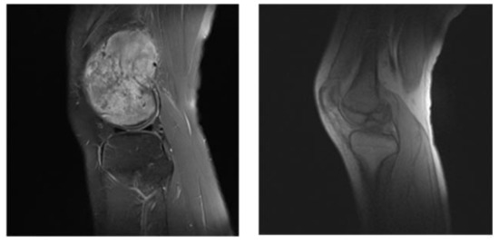
Figure 7.
US (the left) and NS (the right) example images.
After classifying the dataset, we proceeded with data enhancement processing. The effect of data enhancement processing is shown in Figure 8, where the left column is the original label, the middle column is the segmentation rendering without optimization processing, and the right column is the optimized segmentation renderings. We can see that there is an incomplete and inaccurate segmentation in the middle column, and after optimization, the segmentation can obtain a relatively complete and accurate tumor region prediction. From here we can see that after the data optimization, the performance of the model has been significantly improved.
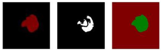
Figure 8.
The renderings before and after preprocessing.
Figure 9 shows the effect of each model on the segmentation of osteosarcoma MRI images. Among them, from left to right are the segmentation renderings of the label image, our model, FCN16, FCN8, FPN, MSFCN, MSRN, and U-net. We can visually compare the performance differences of the models through the segmentation effects of each model. According to the comparison of the selected six osteosarcoma segmentation instances, it can be seen that our model has a good segmentation effect and can more accurately divide the lesion area, while other models may have insufficient segmentation (such as MSFCN) and excessive segmentation, partitioning (such as FPN) and other issues.
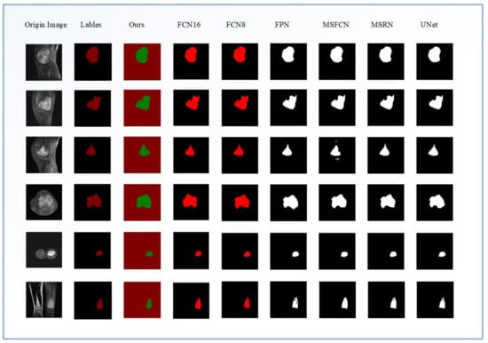
Figure 9.
The effects of different segmentation models for osteosarcoma MRI images.
In order to evaluate the performance of each model in more detail, we quantitatively compare the parameters of the segmentation methods and analyze the models from different evaluation indicators. Table 3 lists the parameters of different methods on the osteosarcoma dataset in detail to reflect the performance difference of different segmentation methods. From the table, we can see that our FaBiNet segmentation model performs very well in the task of segmenting osteosarcoma, and its DSC, IoU, Recall and other indicators are at the forefront, with excellent performance. While achieving such accuracy, the parameter scale of the model is far smaller than other models, so the performance requirements for hardware are very low, and there is no need for grassroots hospitals and other organizations to be equipped with expensive computing equipment, which further saves costs and is conducive to the popularization of the system.
Table 3.
Index parameter values of different methods.
Figure 10 below is a comparison chart of the DSC of different segmentation models and the number of parameters of this model. From the results, we can see that the DSC of our proposed osteosarcoma segmentation method is the highest, reaching 0.915, which is higher than the second-place UNet; this reflects the high segmentation accuracy of our model, and the segmentation accuracy is guaranteed. At the same time, the number of parameters of our model is far more effective than other models. The params is only 2.33 M, while ensuring accuracy, and the degree of lightweight is also very high. It greatly reduces the difficulty of training, so that our osteosarcoma auxiliary recognition system can run smoothly on low-cost hardware.
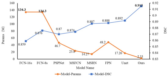
Figure 10.
The DSC for different models and parameter scale for this model.
Figure 11 depicts a legend for the comparison of the IoU and the parameter scale for different models. From the figure, we can see that the IoU of each segmentation model is relatively high. Except for PSPNet, the IoU of other models is above 0.8. And the IoU of our FaBiNet is second only to Unet; the former is 0.853, and the latter is 0.867. The difference between the two is also very small. However, we can see from the figure that under the premise that the IoU gap is not large, the params gap of each model is more obvious. Among them, our model param is only 2.33 M, and the parameter value of Unet whose IoU is slightly higher than that of FaBiNet is 17.26 M. For example, with FCN, when it reaches an IoU of about 0.83, the parameter scale reaches an astonishing 134.3 M, which means that the model is too complicated, so it is not conducive to practical use.
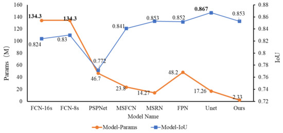
Figure 11.
Comparison of IoU and parameter scale of different models.
Figure 12 below shows how the accuracy of each model’s changes as training progresses. We trained a total of 1000 epochs, and randomly selected 50 epochs (20 random epochs to choose one epoch) for comparison and analysis. It can be seen from the line chart that after 200 rounds of training, the accuracy of each model tends to be stable; numerically, the accuracy rate of our FaBiNet is the highest, reaching 96% in steady state, and the highest accuracy is more than 98%. The accuracy rate and stability are both at an excellent level. In terms of accuracy, the ranking of each model is: FaBiNet (Ours) > UNet > FPN > FCN-8s ≈ FCN-16s > MSRN > MSFCN.
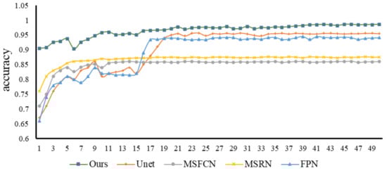
Figure 12.
Accuracy changes of each model.
Recall is an important evaluation index in tumor image recognition. If the recall fluctuation of a model is relatively small and the value is high when it is stable, then this model not only has a high recognition rate, but also avoids the occurrence of missed diagnosis as much as possible. From Figure 13, we can observe the recall trends and values of various models. We can see that in the first 220 epochs of training, the recall fluctuations of the Unet, FPN, and MSFCN models are relatively large. After that, most of the models have stabilized. Generally speaking, the recall of our model is relatively high and relatively stable, and there will be no big fluctuations in the early stage, so the performance is excellent. Subsequently, we selected the same four models to compare with our model and study their F1-score relationship. From Figure 14 of epoch—F1-score, we can see that the F1-score of our model is always kept at a high level, and the stability is also better, which indicates that our model has better robustness.
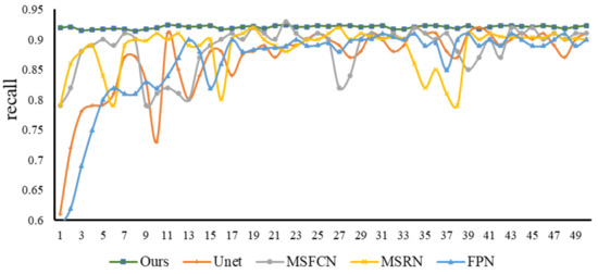
Figure 13.
Recall changes of each model.
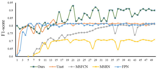
Figure 14.
F1-score changes of each model.
5. Conclusions
Using more than 80,000 MRI images of osteosarcoma from three hospitals in China as a dataset, this paper proposes an osteosarcoma-assisted segmentation method based on guided aggregation bilateral networks. In this method, we first optimized the dataset, then preprocessed the images, and finally performed image segmentation. Due to the unique architecture of our segmentation model, it can achieve high recognition rates with a low parameter scale. Comparing our method with other image segmentation algorithms, the experimental results show that our method has better segmentation performance. At the same time, our model is highly lightweight and can be easily deployed on low-cost devices. This reduces the cost of hardware facilities.
With the rapid development of information technology, we can further expand our data set, make certain improvements to the model, design a more scientific and effective training process, and optimize the segmentation edges to further improve the effect of segmentation. We are committed to improving our model and making it more mature so as to reduce the burden on front-line clinicians around the world and to contribute to the auxiliary diagnosis of osteosarcoma.
Author Contributions
Methodology, Y.S., F.G. and Z.D.; validation, Y.S., F.G. and Z.D.; writing—original draft preparation, Y.S., F.G. and Z.D.; writing—review and editing, Y.S., F.G. and Z.D.; visualization, Y.S., F.G. and Z.D. All authors have read and agreed to the published version of the manuscript.
Funding
This work was supported in the Hunan Provincial Natural Science Foundation of 690 China (2018JJ3299, 2018JJ3682, 2019JJ40440).
Institutional Review Board Statement
Not applicable.
Informed Consent Statement
Not applicable.
Data Availability Statement
Data used to support the findings of this study are currently under embargo while the research findings are commercialized. Requests for data, 12 months after publication of this article, will be considered by the corresponding author.
Conflicts of Interest
The authors declare that they have no conflicts of interest.
References
- Yu, G.; Wu, J. Efficacy prediction based on attribute and multi-source data collaborative for auxiliary medical system in developing countries. Neural Comput. Appl. 2022, 34, 5497–5512. [Google Scholar] [CrossRef]
- Li, X.; Qi, H.; Wu, J. Efficient path-sense transmission based on IoT system in opportunistic social networks. Peer-to-Peer Netw. Appl. 2022, 15, 811–826. [Google Scholar] [CrossRef]
- Wu, J.; Yang, S.; Gou, F.; Zhou, Z.; Xie, P.; Xu, N.; Dai, Z. Intelligent Segmentation Medical Assistance System for MRI Images of Osteosarcoma in Developing Countries. Comput. Math. Methods Med. 2022, 2022, 7703583. [Google Scholar] [CrossRef]
- Wu, J.; Gou, F.; Tian, X. Disease Control and Prevention in Rare Plants Based on the Dominant Population Selection Method in Opportunistic Social Networks. Comput. Intell. Neurosci. 2022, 2022, 1489988. [Google Scholar] [CrossRef] [PubMed]
- Gou, F.; Wu, J. Message Transmission Strategy Based on Recurrent Neural Network and Attention Mechanism in Iot System. J. Circuits, Syst. Comput. 2022, 31, 2250126. [Google Scholar] [CrossRef]
- Wu, J.; Gou, F.; Xiong, W.; Zhou, X. A Reputation Value-Based Task-Sharing Strategy in Opportunistic Complex Social Networks. Complexity 2021, 2021, 8554351. [Google Scholar] [CrossRef]
- Wu, J.; Qu, J.; Yu, G. Behavior prediction based on interest characteristic and user communication in opportunistic social networks. Peer-to-Peer Netw. Appl. 2021, 14, 1006–1018. [Google Scholar] [CrossRef]
- Ouyang, W.; Chen, Z.; Wu, J.; Yu, G.; Zhang, H. Dynamic Task Migration Combining Energy Efficiency and Load Balancing Optimization in Three-Tier UAV-Enabled Mobile Edge Computing System. Electronics 2021, 10, 190. [Google Scholar] [CrossRef]
- Wu, J.; Gou, F.; Tan, Y. A staging auxiliary diagnosis model for non-small cell lung cancer based the on intelligent medical system. Comput. Math. Methods Med. 2021, 2021, 6654946. [Google Scholar] [CrossRef]
- Dong, Y.; Chang, L.; Luo, J.; Wu, J. A Routing Query Algorithm Based on Time-Varying Relationship Group in Opportunistic Social Networks. Electronics 2021, 10, 1595. [Google Scholar] [CrossRef]
- Deng, Y.; Gou, F.; Wu, J. Hybrid data transmission scheme based on source node centrality and community reconstruction in opportunistic social networks. Peer-to-Peer Netw. Appl. 2021, 14, 3460–3472. [Google Scholar] [CrossRef]
- Wu, J.; Zou, W.; Long, H. Effective path prediction and data transmission in opportunistic social networks. IET Commun. 2021, 15, 2202–2211. [Google Scholar] [CrossRef]
- Gou, F.; Wu, J. Triad link prediction method based on the evolutionary analysis with IoT in opportunistic social networks. Comput. Commun. 2021, 181, 143–155. [Google Scholar] [CrossRef]
- Xu, Y.; Chen, Z.G.; Wu, J.; Yu, G. MNSRQ: Mobile node social relationship quantification algorithm for data transmission in Internet of things. IET Commun. 2021, 15, 748–761. [Google Scholar] [CrossRef]
- Lu, Y.; Chang, L.; Luo, J.; Wu, J. Routing Algorithm Based on User Adaptive Data Transmission Scheme in Opportunistic Social Networks. Electronics 2021, 10, 1138. [Google Scholar] [CrossRef]
- Cui, R.; Chen, Z.; Wu, J.; Tan, Y.; Yu, G. A Multiprocessing Scheme for PET Image Pre-Screening, Noise Reduction, Segmentation and Lesion Partitioning. IEEE J. Biomed. Heal. Inform. 2021, 25, 1699–1711. [Google Scholar] [CrossRef]
- Zhang, X.; Chang, L.; Luo, J.; Wu, J. Effective communication data transmission based on community clustering in opportunistic social networks in IoT system. J. Intell. Fuzzy Syst. 2021, 41, 2129–2144. [Google Scholar] [CrossRef]
- Nasor, M.; Obaid, W. Segmentation of osteosarcoma in MRI images by K-means clustering, Chan-Vese segmentation, and iterative Gaussian filtering. IET Image Process. 2020, 15, 1310–1318. [Google Scholar] [CrossRef]
- Shuai, L.; Gao, X.; Wang, J. Wnet ++: A Nested W-shaped Network with Multiscale Input and Adaptive Deep Supervision for Osteosarcoma Segmentation. In Proceedings of the 2021 IEEE 4th International Conference on Electronic Information and Communication Technology (ICEICT), Xi’an, China, 18–20 August 2021. [Google Scholar] [CrossRef]
- Zhang, R.; Huang, L.; Xia, W.; Zhang, B.; Qiu, B.; Gao, X. Multiple supervised residual network for osteosarcoma segmentation in CT images. Comput. Med. Imaging Graph. 2018, 63, 1–8. [Google Scholar] [CrossRef]
- Arunachalam, H.B.; Mishra, R.; Daescu, O.; Cederberg, K.; Rakheja, D.; Sengupta, A.; Leonard, D.; Hallac, R.; Leavey, P. Viable and necrotic tumor assessment from whole slide images of osteosarcoma using ma-chine-learning and deep-learning models. PLoS ONE 2019, 14, e0210706. [Google Scholar] [CrossRef]
- Nabid, R.A.; Rahman, M.L.; Hossain, M.F. Classification of Osteosarcoma Tumor from Histological Image Using Sequential RCNN. In Proceedings of the 2020 11th International Conference on Electrical and Computer Engineering (ICECE), Dhaka, Bangladesh, 17–19 December 2020. [Google Scholar]
- Fu, Y. Deep Model with Siamese Network for Viability and Necrosis Tumor Assessment in Osteosarcoma. arXiv 2019, arXiv:1910.12513. [Google Scholar]
- Qiao, Y.-J.; Gao, B.-L.; Shi, R.-X.; Liu, X.; Wang, Z.-H. Improved FCM Brain MRI Image Segmentation Algorithm Based on Tamura Texture Feature. Ji Suan Ji Ke Xue 2021, 48, 111–117. [Google Scholar]
- Hua, L.; Gu, Y.; Gu, X.; Xue, J.; Ni, T. A Novel Brain MRI Image Segmentation Method Using an Improved Multi-View Fuzzy c-Means Clustering Algorithm. Front. Neurosci. 2021, 15, 662674. [Google Scholar] [CrossRef] [PubMed]
- Tarkhaneh, O.; Shen, H. An adaptive differential evolution algorithm to optimal multi-level thresholding for MRI brain image segmentation. Expert Syst. Appl. 2019, 138, 112820. [Google Scholar] [CrossRef]
- Sasikala, E.; Kanmani, P.; Gopalakrishnan, R.; Radha, R. Identification of lesion using an efficient hybrid algorithm for MRI brain image segmentation. J. Ambient Intell. Humaniz. Comput. 2021. [Google Scholar] [CrossRef]
- Anisuzzaman, D.; Barzekar, H.; Tong, L.; Luo, J.; Yu, Z. A deep learning study on osteosarcoma detection from histological images. Biomed. Signal Process. Control 2021, 69, 102931. [Google Scholar] [CrossRef]
- Chen, H.; Zhang, X.; Wang, X.; Quan, X.; Deng, Y.; Lu, M.; Wei, Q.; Ye, Q.; Zhou, Q.; Xiang, Z.; et al. MRI-based radiomics signature for pretreatment prediction of pathological response to neoadjuvant chemo-therapy in osteosarcoma: A multicenter study. Eur. Radiol. 2021, 31, 7913–7924. [Google Scholar] [CrossRef]
- Dionísio, F.; Oliveira, L.; Hernandes, M.; Engel, E.; Rangayyan, R.; Azevedo-Marques, P.; Nogueira-Barbosa, M. Manual and semiautomatic segmentation of bone sarcomas on MRI have high similarity. Braz. J. Med Biol. Res. 2020, 53, e8962. [Google Scholar] [CrossRef] [PubMed] [Green Version]
- Baidya Kayal, E.; Kandasamy, D.; Sharma, R.; Sharma, M.C.; Bakhshi, S.; Mehndiratta, A. SLIC-supervoxels-based response evaluation of osteosarcoma treated with neoadjuvant chemother-apy using multi-parametric MR imaging. Eur. Radiol. 2020, 30, 3125–3136. [Google Scholar] [CrossRef]
- Dai, Y.; Yin, P.; Mao, N.; Sun, C.; Wu, J.; Cheng, G.; Hong, N. Differentiation of Pelvic Osteosarcoma and Ewing Sarcoma Using Radiomic Analysis Based on T2-Weighted Images and Contrast-Enhanced T1-Weighted Images. BioMed Res. Int. 2020, 2020, 9078603. [Google Scholar] [CrossRef]
- Parlak, Ş.; Ergen, F.B.; Yüksel, G.Y.; Karakaya, J.; Aydın, G.B.; Kösemehmetoğlu, K.; Aydıngöz, Ü. Diffusion-weighted imaging for the differentiation of Ewing sarcoma from osteosarcoma. Skelet. Radiol. 2021, 50, 2023–2030. [Google Scholar] [CrossRef] [PubMed]
- Barnett, J.R.; Gikas, P.; Gerrand, C.; Briggs, T.W.; Saifuddin, A. The sensitivity, specificity, and diagnostic accuracy of whole-bone MRI for identifying skip metastases in appendicular osteosarcoma and Ewing sarcoma. Skelet. Radiol. 2020, 49, 913–919. [Google Scholar] [CrossRef] [PubMed]
- Guerra, R.B.; Tostes, M.D.; Miranda LD, C.; Camargo OP, D.; Baptista, A.M.; Caiero, M.T.; dos Santos Machado, T.M.; Abadi, M.D.; de Oliveira, C.R.G.C.M.M.; Filippi, R.Z. Comparative analysis between osteosarcoma and Ewing’s sarcoma: Evaluation of the time from onset of signs and symptoms until diagnosis. Clinics 2006, 61, 99–106. [Google Scholar] [CrossRef] [PubMed] [Green Version]
- Zhan, X.; Long, H.; Gou, F.; Duan, X.; Kong, G.; Wu, J. A Convolutional Neural Network-Based Intelligent Medical System with Sensors for Assistive Diagnosis and Decision-Making in Non-Small Cell Lung Cancer. Sensors 2021, 21, 7996. [Google Scholar] [CrossRef] [PubMed]
- Long, J.; Shelhamer, E.; Darrell, T. Fully convolutional networks for semantic segmentation. In Proceedings of the IEEE Conference on Computer Vision and Pattern Recognition, Boston, MA, USA, 7–12 June 2015; pp. 3431–3440. [Google Scholar] [CrossRef] [Green Version]
- Zhao, H.; Shi, J.; Qi, X.; Wang, X.; Jia, J. Pyramid scene parsing network. In Proceedings of the 2017 IEEE Conference on Computer Vision and Pattern Recognition, Honolulu, HI, USA, 21–26 July 2017; pp. 2881–2890. [Google Scholar] [CrossRef] [Green Version]
- Huang, L.; Xia, W.; Zhang, B.; Qiu, B.; Gao, X. MSFCN-multiple supervised fully convolutional networks for the osteosarcoma segmentation of CT images. Comput. Methods Programs Biomed. 2017, 143, 67–74. [Google Scholar] [CrossRef] [PubMed]
- Ronneberger, O.; Fischer, P.; Brox, T. U-Net: Convolutional networks for biomedical image segmentation. In Medical Image Computing and Computer-Assisted Intervention 2015; Navab, N., Hornegger, J., Wells, W.M., Frangi, A.F., Eds.; Springer International Publishing: Cham, Switzerland, 2015; pp. 234–241. [Google Scholar] [CrossRef] [Green Version]
- Lin, T.Y.; Dollár, P.; Girshick, R.; He, K.; Hariharan, B.; Belongie, S. Feature pyramid networks for object detection. In Proceedings of the 2017 IEEE Conference on Computer Vision and Pattern Recognition (CVPR), Honolulu, HI, USA, 21–26 July 2017; pp. 936–944. [Google Scholar] [CrossRef] [Green Version]
Publisher’s Note: MDPI stays neutral with regard to jurisdictional claims in published maps and institutional affiliations. |
© 2022 by the authors. Licensee MDPI, Basel, Switzerland. This article is an open access article distributed under the terms and conditions of the Creative Commons Attribution (CC BY) license (https://creativecommons.org/licenses/by/4.0/).