Construction of Cubic Trigonometric Curves with an Application of Curve Modelling

Abstract

This paper introduces new trigonometric basis functions (TBF) in polynomial and rational form with two shape parameters (SPs). Some classical characteristics, such as the partition of unity, positivity, symmetry, CHP, local control and invariance under affine transformation properties are proven mathematically and graphically. In addition, different continuity conditions at uniform knots (UK) are proven. Some open and closed curves from TBS and trigonometric rational B-spline (TRBS) are generated to test the applicability of the suggested technique, and the influence of the shape parameter is also noted. Furthermore, various objects, such as designing an alphabet, star, butterfly, leaf and 3D cube.

1. Introduction

In CAGD, B-spline is an important ingredient in geometric modelling, and the role of TBS is seen to be crucial for the designing and manipulation of geometrical curves and surfaces. Many schemes have been developed for the curve designing. These include ordinary Bézier [1,2], Ball Bézier-like [3], H-Bézier [4], Q-Bézier [5], classical B-spline [1,2] and non-uniform rational basis spline (NURBS) [1,2] etc. The comparison of Harmonic rational curves with p-Bézier curves was proposed in [6]. $C^2$ Algebraic-Trigonometric Pythagorean Hodograph (ATPH) splines were created in [7] by solving a non-linear system of equations in complex variables.

The problem of $G^1$ Hermite interpolation by PH cubic segments was proposed in [8]. In [9], Zhu and Han constructed a new trigonometric Bernstein basis, such as functions with two exponential SPs, and they proved that the cubic trigonometric Bézier-like curves were more efficient than the cubic Bézier curves. Various trigonometric Bézier-like functions in [10,11] have been implemented in recent years. The relationship between the two shape parameters and their geometric effect on the curve is discussed in [12]. These shape parameters are self-contained and thus demonstrated that their geometric effect on the curve is linear.

In [13], a new basis called the C-Bézier basis was presented. This shows that such a basis and curves in polynomial spaces are similar to the Bernstein basis and Bézier curves. Chen et al. [14] built a new generalisation of the Bernstein operator based on a non-negative real parameter. The shape-preserving properties of generalised Bernstein operators are also investigated. They demonstrated that monotonic or convex functions result in monotonic or convex generalised Bernstein polynomials. The q-Bernstein polynomials, which generalise the conventional Bernstein polynomials, were described by [15], who showed that the difference between two successive q-Bernstein polynomials of a function f may be represented in terms of second-order split differences of f.

With respect to the Jacobi $L_2$-norm proposed in [16], a weighted least-squares approximation of Bézier coefficients with factored Hahn weights provides the best constrained polynomial degree reduction. Whereas, by constructing bivariate Bernstein–Kantorovich type operators on an extended domain with reparametrized knots, a link between approximation theory and summability methods was established in [17].

In [18], Schoenberg introduced the trigonometric splines with a recurrence relation. The geometric effect of the shape parameter on curves and the investigation on the Constrained modification of the curves is discussed in [19]. The author defined that spline curves are types of curves that are equitably unite, i.e., significantly, a set of two or more polynomials. Splines are widely used in many fields of engineering, such as data fitting. In [20] the proposed method can be used to fit any type of curve ranging from smooth to discontinuous.

Furthermore, the method does not necessitate a high computational cost, thus, allowing it to be used in automatic reverse engineering applications. Han [21] constructed quadratic TBS curves and compared these to quadratic B-spline curves; they were smoother and closer to a control polygon. The authors in [22,23] introduced the term B-spline (Basis spline). In the mid-1980s, curves swarmed the field of Computer Aided Geometric Design (CAGD). Choubey and Ojha [24] developed TBS with one SP. In [25], the author contributed to the literature by proposing cubic TBS curves on uniform and non-UK with SPs. Yan [26] showed how to create a class of NURBS basis functions having a single SP. For a single knot, $C^2$ continuity can be achieved, and $C^3$ and $C^5$ continuity can be attained using the proposed basis for a unique SP.

A new class of algebraic trigonometric blended spline curves created over space were proposed in [27]. The SPs x and y in the proposed curve are used to control the curve. For the designing of rational surfaces, a scheme based on $\lambda \mu -B$ B-spline was proposed in [28]. This method works well for modifying the complicated structures of rotational surfaces. A technique using a cubic TRBS with two SP as put into practise to construct flexible curves [29]. The sampling method for the reconstruction of curves and surfaces was proposed by [30]. They also discussed how to represent surfaces generated by two or more curves. With an application to curve design, [31] derived certain identities for trigonometric B-splines. In [32], the construction of craniofacial fractures using rational ball curve was introduced, which involves four free parameters. The construction of numerous bone fractures using NURBS curves and CT scan data in the DICOM format is described in [33].

This paper is an attempt to introduce new TBF and TBS curves with SP. The basic geometric properties, such as sum to one, positivity, symmetry, convex hull property and invariance under affine transformation are satisfied by the proposed basis functions. Different continuity conditions at UK were derived for TBF and TRBS functions. The main advantage of using trigonometric B-spline functions is that these functions have built-in continuity. There is no need to derive continuity conditions from segment to segment.

In order to change the curve from any particular point, we need to adjust that point according to our need. The applicability and efficiency of the suggested curves were tested using a variety of open and closed curves. Finally, the suggested curves are applied to 2D and 3D modelling. The main objectives of this paper are:

• To work on cubic TBF using trigonometric Bézier basis functions with some appropriate choice of SP $\lambda$.
• To demonstrate how the form parameter affects TBS basic functions and TBS curves.
• To derive different properties of CTBS along with their continuities in both polynomial and rational form.
• To construct different objects using CTBS and their applications in practical life.

The rest of the research is presented as follows: In Section 2, cubic TBFs are designed, and their geometric characteristics are proven mathematically and graphically as well. Section 3 discusses the construction and validity of cubic TBS curves. Section 4 presents the construction of cubic TRBS basis functions and also proves their basic properties. In Section 5, we elaborate on the design of the TRBS curve and construct open and closed curves by using appropriate values of SP $\lambda$ and weights. The application of CTBS in the geometric modelling of different objects is explained in Section 6. The concluding remarks of this study are given in Section 7.

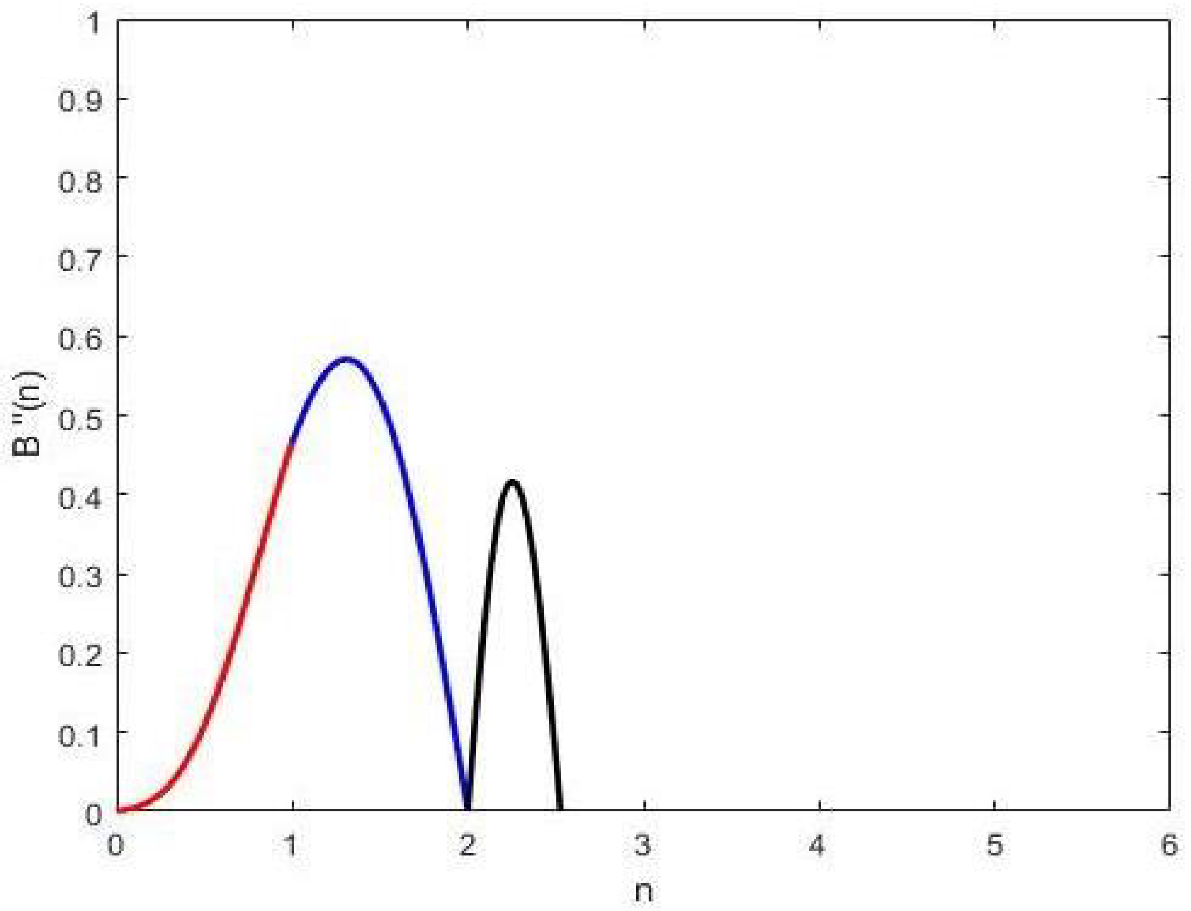
2. Cubic Trigonometric B-Spline Basis Functions

Definition 1.

Consider $N=(n_0,n_1,\dots ..,n_{j+4})$ are the knot vectors in such a way that $n_0<n_1<n_2<\cdots <n_{j+4}$, where j denotes the degree of the curve. The new TBF with the UK are defined as follows.

$$B_i\left(n\right)=\left\{\begin{array}{c}{s}_i\left(b_3\left(u_i\right)\right),n\in [n_i,n_{i+1}),\hfill \\ \sum _{k=0}^3{r}_{i+1,k}(b_k\left(u_{i+1}\right)),n\in [n_{i+1},n_{i+2}),\hfill \\ \sum _{k=0}^3{q}_{i+2,k}(b_k\left(u_{i+2}\right)),n\in [n_{i+2},n_{i+3}),\hfill \\ p_{i+3}\left(b_0\left(u_{i+3}\right)\right),n\in [n_{i+3},n_{i+4}),\hfill \\ 0,Otherwise.\hfill \end{array}\right.$$

(1)

Here, we have $u_i\left(n\right)=\frac{\pi }{2}(\frac{n-n_i}{n_{i+1}-ni})$ for $i\in Z^{+}$,

$$\begin{array}{c}\hfill \begin{array}{cc}\hfill s_i& =\frac{{\alpha }_i{\mu }_i}{{\gamma }_i},r_{i,0}=s_i,r_{i,1}=\frac{{\alpha }_i\Delta n_{i-1}}{{\gamma }_i},\hfill \\ \hfill r_{i,2}& =\frac{{\alpha }_i{\mu }_i}{{\gamma }_i},r_{i,3}=\frac{{\alpha }_i{\gamma }_i{\mu }_i\Delta n_{i+1}+{\alpha }_i{\gamma }_i{\nu }_i\Delta n_i}{{\gamma }_i^2{\beta }_i},\hfill \\ \hfill q_{i,0}& =\frac{{\alpha }_i{\gamma }_i{\mu }_i\Delta n_i+{\alpha }_i{\gamma }_i{\nu }_i\Delta n_{i-1}}{{\beta }_i{\gamma }_i^2},\hfill \\ \hfill q_{i,1}& =\frac{{\alpha }_i{\nu }_i}{{\gamma }_i},q_{i,2}=\frac{{\alpha }_i\Delta n_{i+1}}{{\gamma }_i},\hfill \\ \hfill q_{i,3}& =p_j,p_i=\frac{{\alpha }_i\Delta n_i}{{\beta }_i{\gamma }_i}.\hfill \end{array}\end{array}$$

(2)

where,

$$\begin{array}{c}\hfill \begin{array}{cc}\hfill \Delta n_i& =n_{i+1}-n_i,{\beta }_i=\Delta n_{i-1}+\Delta n_i,\hfill \\ \hfill {\alpha }_i& =1+2{\lambda }_i,{\mu }_i=\Delta n_{i-1}+{\alpha }_i\Delta n_i,{\nu }_i={\alpha }_i\Delta n_{i-1}+\Delta n_i,\hfill \\ \hfill {\gamma }_i& ={\alpha }_i\Delta n_{i-2}+{\alpha }_i^2\Delta n_{i-1}+{\alpha }_i\Delta n_i.\hfill \end{array}\end{array}$$

(3)

with the shape parameter (SP) $\lambda \in [0,1)$ with the proposed TBFs as:

$$\begin{array}{c}\hfill \begin{array}{cc}\hfill b_0(u)& =(1-sin(\frac{\pi }{2})u)(1-sin(\frac{\pi }{2})u+\lambda sin(\frac{\pi }{2})u),\hfill \\ \hfill b_1(u)& =(sin(\frac{\pi }{2})u)(1-sin(\frac{\pi }{2})u)(2-\lambda ),\hfill \\ \hfill b_2(u)& =(cos(\frac{\pi }{2})u)(1-cos(\frac{\pi }{2})u)(2-\lambda ),\hfill \\ \hfill b_3(u)& =(1-cos(\frac{\pi }{2})u)(1-cos(\frac{\pi }{2})u+\lambda cos(\frac{\pi }{2})u).\hfill \end{array}\end{array}$$

(4)

Figure 1 and Figure 2 represent the graphical behaviour of proposed basis functions. In Figure 3, the effect of SP can be observed, and thus this effect is demonstrated using various colours as shown in

Table 1. Different values of shape parameter $\lambda$.

Sr No.	Curves	$\mathit{\lambda }$
1	red	$0.01$
2	black	$0.35$
3	magenta	$0.55$
4	blue	$0.75$

.

Properties of the Basis Functions

Following are the properties that the above cubic TBF satisfies.

Theorem 1.

The given cubic trigonometric basis functions (TBF) satisfy the property of partition of unity—that is, for n as a knot vector and $i=0,1,2,\dots .,j+4$ for j being the degree of the curve, we have

$${\sum }_{i=0}^3{B}_i\left(n\right)=1.$$

Proof. 

For $i\ne (i-3),(i-2),(i-1),\left(i\right)$, we have $B_i\left(n\right)=0$ and $B_i\left(n\right)$ for $i=(i-3)$, $(i-2)$, $(i-1),\left(i\right)$ is given in the form of $B_{i-3}\left(n\right)$, $B_{i-2}\left(n\right)$, $B_{i-1}\left(n\right)$, $B_i\left(n\right)$ is defined as

$$B_{i-3}\left(n\right)=p_i\left(b_0\left(u_i\right)\right),$$

$$B_{i-2}\left(n\right)={\sum }_{k=0}^3{q}_{i,k}{b}_k\left(u_i\right),$$

$$B_{i-1}\left(n\right)={\sum }_{k=0}^3{r}_{i,k}{b}_k\left(u_i\right),$$

$$B_i\left(n\right)=s_i{b}_3\left(u_i\right).$$

The given expression will hold for $n\in [n_i,n_{i+1})$. Here, $u_i\left(n\right)=\frac{\pi }{2}(\frac{n-n_i}{n_{i+1}-ni})$ for $i\in Z^{+}$ and $\lambda \in [0,1)$. Thus, by substituting the values, we find:

$$\begin{array}{ccc}\hfill \sum _{i=i-3}^i{B}_i(n)& =& (\frac{1}{4\lambda +6})(1-sin(\frac{\pi }{2})u_i)(1-sin(\frac{\pi }{2})u_i+\lambda sin(\frac{\pi }{2})u_i)\hfill \\ & & +(\frac{2(1+\lambda )}{2\lambda +3})(1-sin(\frac{\pi }{2})u_i)(1-sin(\frac{\pi }{2})u_i+\lambda sin(\frac{\pi }{2})u_i)\hfill \\ & & +(\frac{2(1+\lambda )}{2\lambda +3})(sin(\frac{\pi }{2})u_i)(1-sin(\frac{\pi }{2})u_i)(2-\lambda )\hfill \\ & & +(\frac{1}{2\lambda +3})(cos(\frac{\pi }{2})u_i)(1-cos(\frac{\pi }{2})u_i)(2-\lambda )\hfill \\ & & +(\frac{1}{4\lambda +6})(1-cos(\frac{\pi }{2})u_i)(1-cos(\frac{\pi }{2})u_i+\lambda cos(\frac{\pi }{2})u_i)\hfill \\ & & +(\frac{1}{4\lambda +6})(1-sin(\frac{\pi }{2})u_i)(1-sin(\frac{\pi }{2})u_i+\lambda sin(\frac{\pi }{2})u_i)\hfill \\ & & +(\frac{1}{2\lambda +3})(sin(\frac{\pi }{2})u_i)(1-sin(\frac{\pi }{2})u_i)(2-\lambda )\hfill \\ & & +(\frac{2(1+\lambda )}{2\lambda +3})(cos(\frac{\pi }{2})u_i)(1-cos(\frac{\pi }{2})u_i)(2-\lambda )\hfill \\ & & +(\frac{2(1+\lambda )}{2\lambda +3})(1-cos(\frac{\pi }{2})u_i)(1-cos(\frac{\pi }{2})u_i+\lambda cos(\frac{\pi }{2})u_i)\hfill \\ & & +(\frac{1}{4\lambda +6})(1-cos(\frac{\pi }{2})u_i)(1-cos(\frac{\pi }{2})u_i+\lambda cos(\frac{\pi }{2})u_i).\hfill \end{array}$$

$$\begin{array}{ccc}\hfill \sum _{i=i-3}^i{B}_i(n)& =& (\frac{1}{4\lambda +6})\{1+(\lambda -2)sin(\frac{\pi }{2})u_i+(1-\lambda ){sin}^2(\frac{\pi }{2})u_i\}\hfill \\ & & +(\frac{2(1+\lambda )}{2\lambda +3})\{1+(\lambda -2)sin(\frac{\pi }{2})u_i+(1-\lambda ){sin}^2(\frac{\pi }{2})u_i\}\hfill \\ & & +(\frac{2(1+\lambda )}{2\lambda +3})\{(2-\lambda )sin(\frac{\pi }{2})u_i+(\lambda -2){sin}^2(\frac{\pi }{2})u_i\}\hfill \\ & & +(\frac{1}{2\lambda +3})\{(2-\lambda )cos(\frac{\pi }{2})u_i+(\lambda -2){cos}^2(\frac{\pi }{2})u_i\}\hfill \\ & & +(\frac{1}{4\lambda +6})\{1+(\lambda -2)cos(\frac{\pi }{2})u_i+(1-\lambda ){cos}^2(\frac{\pi }{2})u_i\}\hfill \\ & & +(\frac{1}{4\lambda +6})\{1+(\lambda -2)sin(\frac{\pi }{2})u_i+(1-\lambda ){sin}^2(\frac{\pi }{2})u_i\}\hfill \\ & & +(\frac{1}{2\lambda +3})\{(2-\lambda )sin(\frac{\pi }{2})u_i+(\lambda -2){sin}^2(\frac{\pi }{2})u_i\}\hfill \\ & & +(\frac{2(1+\lambda )}{2\lambda +3})\{(2-\lambda )cos(\frac{\pi }{2})u_i+(\lambda -2){cos}^2(\frac{\pi }{2})u_i\}\hfill \\ & & +(\frac{2(1+\lambda )}{2\lambda +3})\{1+(\lambda -2)cos(\frac{\pi }{2})u_i+(1-\lambda ){cos}^2(\frac{\pi }{2})u_i\}\hfill \\ & & +(\frac{1}{4\lambda +6})\{1+(\lambda -2)cos(\frac{\pi }{2})u_i+(1-\lambda ){cos}^2(\frac{\pi }{2})u_i\}.\hfill \\ \hfill \sum _{i=i-3}^i{B}_i(n)& =& 2-{sin}^2(\frac{\pi }{2})u_i-{cos}^2(\frac{\pi }{2})u_i.\hfill \end{array}$$

Thus, ${\sum }_{i=i-3}^i{B}_i\left(n\right)=1$. □

Theorem 2.

The given basis functions and the proposed TBFs are positive or zero having the SP $\lambda ,$ i.e., $B_i\left(n\right)\ge 0.$

Proof. 

As the first and last interval consists of one term only, the property is true for both of the intervals. Whereas, for the second interval, let us take $z=tan\left(\frac{1}{2}\right)u$ and $u\in [0,1]$:

$$\begin{array}{ccc}\hfill \sum _{k=0}^3{r}_{i,k}\left(b_k\left(u\right)\right)& =& r_{i,0}\left(b_0\left(u\right)\right)+r_{i,1}\left(b_1\left(u\right)\right)+r_{i,2}\left(b_2\left(u\right)\right)+r_{i,3}\left(b_3\left(u\right)\right).\hfill \\ & =& r_{i,0}\{1+(\lambda -2)sin\left(\frac{\pi }{2}\right)u+(1-\lambda ){sin}^2\left(\frac{\pi }{2}\right)u\}\hfill \\ & & +r_{i,1}\{(2-\lambda )sin\left(\frac{\pi }{2}\right)u+(\lambda -2){sin}^2\left(\frac{\pi }{2}\right)u\}\hfill \\ & & +r_{i,2}\{(2-\lambda )cos\left(\frac{\pi }{2}\right)u+(\lambda -2){cos}^2\left(\frac{\pi }{2}\right)u\}\hfill \\ & & +r_{i,3}\{1+(\lambda -2)cos\left(\frac{\pi }{2}\right)u+(1-\lambda ){cos}^2\left(\frac{\pi }{2}\right)u\}.\hfill \end{array}$$

Now, with

$$\begin{array}{c}\hfill sin\left(\frac{\pi }{2}\right)u=\frac{2z}{1+z^2},andcos\left(\frac{\pi }{2}\right)u=\frac{1-z^2}{1+z^2}.\end{array}$$

We obtain

$$\begin{array}{ccc}\hfill \sum _{k=0}^3{r}_{i,k}\left(b_k\left(u\right)\right)& =& \{\frac{1}{{(1+z^2)}^2}\}(\sum _{k=0}^4{z}_k{y}^k).\hfill \end{array}$$

Here,

$$\begin{array}{ccc}\hfill z_0& =& c_{i,0},\hfill \\ \hfill z_1& =& (2\lambda -4)(r_{i,0}-r_{i,1}),\hfill \\ \hfill z_2& =& (6-4\lambda )r_{i,0}+(4\lambda -8)r_{i,1}-(2\lambda -4)r_{i,2}+\left(2\lambda \right)r_{i,3},\hfill \\ \hfill z_3& =& 2(\lambda -2)(r_{i,0}-r_{i,1}),\hfill \\ \hfill z_4& =& c_{i,0}+2(\lambda -2)(r_{i,2}-r_{i,3}).\hfill \end{array}$$

In the same manner, we can prove this property of $n\in [n_{i+2},n_{i+3})$. □

Theorem 3.

For $B_i(n,\lambda )=B_{3-i}(1-n,\lambda )$ for $i=0,1,2,3$.

Proof. 

For $\lambda \in [0,1)$, we have

$$\begin{array}{c}\hfill sin(\frac{\pi }{2})u\ge 0,1-sin(\frac{\pi }{2})u\ge 0,1-sin(\frac{\pi }{2})u+\lambda sin(\frac{\pi }{2})u\ge 0.\end{array}$$

and

$$\begin{array}{c}\hfill cos(\frac{\pi }{2})u\ge 0,1-cos(\frac{\pi }{2})u\ge 0,1-cos(\frac{\pi }{2})u+\lambda cos(\frac{\pi }{2})u\ge 0.\end{array}$$

Therefore,

$$\begin{array}{c}\hfill \{1+(\lambda -2)sin(\frac{\pi }{2})u+(1-\lambda ){sin}^2(\frac{\pi }{2})u\}=(1-sin(\frac{\pi }{2})u)(1-sin(\frac{\pi }{2})u+\lambda sin(\frac{\pi }{2})u)\ge 0.\end{array}$$

Similarly, we have

$$\begin{array}{c}\hfill \{1+(\lambda -2)cos(\frac{\pi }{2})u+(1-\lambda ){cos}^2(\frac{\pi }{2})u\}=(1-cos(\frac{\pi }{2})u)(1-cos(\frac{\pi }{2})u+\lambda cos(\frac{\pi }{2})u)\ge 0.\\ \hfill \{(2-\lambda )sin(\frac{\pi }{2})u+(\lambda -2){sin}^2(\frac{\pi }{2})u\}=(sin(\frac{\pi }{2})u)(1-sin(\frac{\pi }{2})u)(2-\lambda )\ge 0.\\ \hfill \{(2-\lambda )cos(\frac{\pi }{2})u+(\lambda -2){cos}^2(\frac{\pi }{2})u\}=(cos(\frac{\pi }{2})u)(1-cos(\frac{\pi }{2})u)(2-\lambda )\ge 0.\end{array}$$

□

The symmetry of the given cubic TBS basis functions is shown in Figure 4.

Theorem 4.

For uniform knots (UK), the proposed basis functions are $C^2$ continuous. Now, let $n_{i+1}^{+}$ and $n_{i+1}^{-}$ are the knot vectors in $n\in [n_{i+1},n_{i+2})$, respectively.

Proof. 

For the first interval, the left and right hand continuity is given as

Derivatives at knot$n_{i+1}^{-}$

$$\begin{array}{ccc}\hfill B_i(n_{i+1}^{-})& =& s_i.\hfill \\ \hfill B_i^{\prime }(n_{i+1}^{-})& =& (\frac{\pi }{2\Delta n_i})(2-\lambda )s_j.\hfill \\ \hfill B_i^{″}(n_{i+1}^{-})& =& \frac{1}{2}{(\frac{\pi }{2\Delta n_i})}^2(1-\lambda )s_i.\hfill \\ \hfill B_i^{‴}(n_{i+1}^{-})& =& {(\frac{\pi }{2\Delta n_i})}^3(\lambda -2)s_i.\hfill \\ \hfill B_i^{iv}(n_{i+1}^{-})& =& {(\frac{\pi }{2\Delta n_i})}^4\left\{8(\lambda -1)s_i\right\}.\hfill \\ \hfill B_i^v(n_{i+1}^{-})& =& {(\frac{\pi }{2\Delta n_i})}^5\left\{(2-\lambda )s_i\right\}.\hfill \end{array}$$

Derivatives at knot$n_{i+1}^{+}$

$$\begin{array}{ccc}\hfill B_i(n_{i+1}^{+})& =& r_{i+1,0}=s_{i+1}.\hfill \\ \hfill B_i^{\prime }(n_{i+1}^{+})& =& (\frac{\pi }{2\Delta n_{i+1}})\left\{(\lambda -2)(r_{i+1,0}-r_{i+1,1})\right\}.\hfill \\ \hfill B_i^{″}(n_{i+1}^{+})& =& {(\frac{\pi }{2\Delta n_{i+1}})}^2\{-2(\lambda -1)r_{i+1,0}+(2-\lambda )(r_{i+1,2}-2r_{i+1,1})+\lambda r_{i+1,3}\}.\hfill \\ \hfill B_i^{‴}(n_{i+1}^{+})& =& {(\frac{\pi }{2\Delta n_{i+1}})}^3\left\{(2-\lambda )(r_{i+1,0}-r_{i+1,1})\right\}.\hfill \\ \hfill B_i^{iv}(n_{i+1}^{+})& =& {(\frac{\pi }{2\Delta n_{i+1}})}^4\{8(\lambda -1)r_{i+1,0}+(2-\lambda )(8r_{i+1,1}-7r_{i+1,2})+(6-7\lambda )r_{i+1,3}\}.\hfill \\ \hfill B_i^v(n_{i+1}^{+})& =& ({\frac{\pi }{2\Delta n_{i+1}}}^5)\left\{(\lambda -2)(r_{i+1,0}-r_{i+1,1})\right\}.\hfill \end{array}$$

Derivatives at knot$n_{i+2}^{-}$

$$\begin{array}{ccc}\hfill B_i(n_{i+2}^{-})& =& r_{i+1,3}.\hfill \\ \hfill B_i^{\prime }(n_{i+2}^{-})& =& (\frac{\pi }{2\Delta n_{i+1}})\left\{(2-\lambda )(r_{i+1,3}-r_{i+1,2})\right\}.\hfill \\ \hfill B_i^{″}(n_{i+2}^{-})& =& {(\frac{\pi }{2\Delta n_{i+1}})}^2\{\lambda (r_{i+1,0})+(2-\lambda )(r_{i+1,1}-2r_{i+1,2})+2(1-\lambda )(r_{i+1,3})\}.\hfill \\ \hfill B_i^{‴}(n_{i+2}^{-})& =& {(\frac{\pi }{2\Delta n_{i+1}})}^3\left\{(\lambda -2)(r_{i+1,3}-r_{i+1,2})\right\}.\hfill \\ \hfill B_i^{iv}(n_{i+2}^{-})& =& {(\frac{\pi }{2\Delta n_{i+2}})}^4\{(6-7\lambda )(r_{i+1,0})+(2-\lambda )(8r_{i+1,2}-7r_{i+1,1})+8(\lambda -1)(r_{i+1,3})\}.\hfill \\ \hfill B_i^v(n_{i+2}^{-})& =& {(\frac{\pi }{2\Delta n_{i+1}})}^5\left\{(2-\lambda )(r_{i+1,2}-r_{i+1,3})\right\}.\hfill \end{array}$$

Derivatives at knot$n_{i+2}^{+}$

$$\begin{array}{ccc}\hfill B_i(n_{i+2}^{+})& =& q_{i+2,0}.\hfill \\ \hfill B_i^{\prime }(n_{i+2}^{+})& =& (\frac{\pi }{2\Delta n_{i+2}})\left\{(\lambda -2)(q_{i+2,0}-q_{i+2,1})\right\}.\hfill \\ \hfill B_i^{″}(n_{i+2}^{+})& =& {(\frac{\pi }{2\Delta n_{i+2}})}^2\{-2(\lambda -1)q_{i+2,0}+(2-\lambda )(q_{i+2,2}-2q_{i+2,1})+\lambda (q_{i+2,3})\}.\hfill \\ \hfill B_i^{‴}(n_{i+2}^{+})& =& {(\frac{\pi }{2\Delta n_{i+2}})}^3\left\{(2-\lambda )(q_{i+2,0}-q_{i+2,1})\right\}.\hfill \\ \hfill B_i^{iv}(n_{i+2}^{+})& =& {(\frac{\pi }{2\Delta n_{i+2}})}^4\{8(\lambda -1)q_{i+2,0}+(2-\lambda )(8q_{i+2,1}-7q_{i+2,2})+(6-7\lambda )q_{i+2,3}\}.\hfill \\ \hfill B_i^v(n_{i+2}^{+})& =& ({\frac{\pi }{2\Delta n_{i+2}}}^5)\left\{(\lambda -2)(q_{i+2,0}-q_{i+2,1})\right\}.\hfill \end{array}$$

Derivatives at knot$n_{i+3}^{-}$

$$\begin{array}{ccc}\hfill B_i(n_{i+3}^{-})& =& q_{i+2,3}.\hfill \\ \hfill B_i^{\prime }(n_{i+3}^{-})& =& (\frac{\pi }{2\Delta n_{i+2}})\left\{(2-\lambda )(q_{i+2,3}-q_{i+2,2})\right\}.\hfill \\ \hfill B_i^{″}(n_{i+3}^{-})& =& {(\frac{\pi }{2\Delta n_{i+2}})}^2\{\lambda (q_{i+2,0})+(2-\lambda )(q_{i+2,1}-2q_{i+2,2})+2(1-\lambda )(q_{i+2,3})\}.\hfill \\ \hfill B_i^{‴}(n_{i+3}^{-})& =& {(\frac{\pi }{2\Delta n_{i+2}})}^3\left\{(\lambda -2)(q_{i+2,3}-q_{i+2,2})\right\}.\hfill \\ \hfill B_i^{iv}(n_{i+3}^{-})& =& {(\frac{\pi }{2\Delta n_{i+2}})}^4\{(6-7\lambda )(q_{i+2,0})+(2-\lambda )(8q_{i+2,2}-7q_{i+2,1})+8(\lambda -1)(q_{i+2,3})\}.\hfill \\ \hfill B_i^v(n_{i+3}^{-})& =& {(\frac{\pi }{2\Delta n_{i+2}})}^5\left\{(2-\lambda )(q_{i+2,2}-q_{i+2,3})\right\}.\hfill \end{array}$$

Derivatives at knot$n_{i+3}^{+}$

$$\begin{array}{ccc}\hfill B_i(n_{i+3}^{+})& =& p_{i+3}.\hfill \\ \hfill B_i^{\prime }(n_{i+3}^{+})& =& (\frac{\pi }{2\Delta n_{i+3}})\left\{(\lambda -2)(p_{i+3})\right\}.\hfill \\ \hfill B_i^{″}(n_{i+3}^{+})& =& {(\frac{\pi }{2\Delta n_{i+3}})}^2\left\{2(1-\lambda )(p_{i+3})\right\}.\hfill \\ \hfill B_i^{‴}(n_{i+3}^{+})& =& {(\frac{\pi }{2\Delta n_{i+3}})}^3\left\{(2-\lambda )(p_{i+3})\right\}.\hfill \\ \hfill B_i^{iv}(n_{i+3}^{+})& =& {(\frac{\pi }{2\Delta n_{i+3}})}^4\left\{8(\lambda -1)(p_{i+3})\right\}.\hfill \\ \hfill B_i^v(n_{i+3}^{+})& =& {(\frac{\pi }{2\Delta n_{i+3}})}^5\left\{(2-\lambda )(p_{i+3})\right\}.\hfill \end{array}$$

□

The graphical representation of second derivative of proposed basis function is given in Figure 5 for clarification of $C^2$ continuity.

3. Cubic Trigonometric B-Spline Curve

Definition 2.

The cubic trigonometric B-spline (TBS) curve of degree j defined on the control points, such as $C_i(i=0,1,2,\dots .,n)$ in $R^2$ or $R^3$ with UK vectors $N=(n_0,n_1,\dots ,n_{j+4})$, i.e.,

$$\begin{array}{ccc}\hfill H\left(n\right)& =& \sum _{i=0}^n{B}_i\left(n\right)C_i.\hfill \end{array}$$

(5)

As $u_i\left(n\right)=\frac{\pi }{2}(\frac{n-n_i}{n_{i+1}-n_i})$ for $i=0,1,2,3$, the cubic trigonometric curve for $n\in [n_i,n_{i+1})$ is given as

$$\begin{array}{ccc}\hfill H\left(n\right)& =& B_0\left(n\right)C_0+B_1\left(n\right)C_1+B_2\left(n\right)C_2+B_3\left(n\right)C_3.\hfill \end{array}$$

In addition,

$$\begin{array}{ccc}\hfill H\left(n\right)& =& B_{i-3}\left(n\right)C_{i-3}+B_{i-2}\left(n\right)C_{i-2}+B_{i-1}\left(n\right)C_{i-1}+B_i\left(n\right)C_i.\hfill \end{array}$$

Furthermore, Figure 6 shows the cubic TBS curve with a suitable choice of shape parameter (SP) and here,

$$\begin{array}{ccc}\hfill B_{i-3}\left(n\right)& =& B_0\left(n\right)=p_0\left(b_0\left(u_0\right)\right),\hfill \\ \hfill B_{i-2}\left(n\right)& =& B_1\left(n\right)=\sum _{k=0}^3{q}_{1,k}\left(b_k\left(u_1\right)\right),\hfill \\ \hfill B_{i-1}\left(n\right)& =& B_2\left(n\right)=\sum _{k=0}^3{r}_{1,k}\left(b_k\left(u_2\right)\right),\hfill \\ \hfill B_i\left(n\right)& =& B_3\left(n\right)=s_3\left(b_3\left(u_3\right)\right).\hfill \end{array}$$

3.1. Properties of Cubic Trigonometric B-Spline Curve

The B-spline curve

$$H\left(n\right)={\sum }_{i=0}^n{B}_i\left(n\right)C_i.$$

of degree j defined on the knot vectors $N=(n_0,n_1,\dots ,n_{j+4})$ satisfies the following properties.

• Local Control: The cubic TBS curve has the property of local control i.e., in B-spline curve only that segment will be changed where that particular control point is located. Figure 7 shows that the cubic TBS curve does not pass though the extreme points.
• Convex Hull Property: This property shows that all the points of the cubic TBS curve always lie inside the convex hull of its control polygon, i.e., for $n\in [n_i,n_{i+4})$ CHP is shown below in Figure 8.
• Invariance under affine transformation: Let T be an affine transformation, such as rotation, scaling, transformation and reflection. This implies

  $$T\left({\sum }_{i=0}^m{P}_i{B}_i\left(n\right)\right)={\sum }_{i=0}^{m}T\left(P_i\right)B_i\left(n\right).$$
• Continuity of Trigonometric B-spline Curve: The TBS curve $H_n$ has $C^3$ continuity for UK. Let k be the multiplicity of the knot vectors $n_i$, and then the curve has $C^{3-k}$ continuity. Whereas the continuity at $C^{-1}$ implies that the curve is discontinuous.
  In the knot interval $n\in [n_i,n_{i+1})$, the derivatives are evaluated as follows.
  Derivatives at knot $n_i^{+}$

  $$\begin{array}{ccc}\hfill H(n_i^{+})& =& p_i{C}_{i-3}+q_{i,0}{C}_{i-2}+r_{i,0}{C}_{i-1},\hfill \\ \hfill H^{\prime }(n_i^{+})& =& (\frac{\pi }{2\Delta n_i})\left[(\lambda -2)\{(p_i{C}_{i-3}+q_{i,0}{C}_{i-2}+r_{i,0}{C}_{i-1})-(q_{i,1}{C}_{i-2}+r_{i,1}{C}_{i-1})\}\right],\hfill \\ \hfill H^{″}(n_i^{+})& =& {(\frac{\pi }{2\Delta n_i})}^2[-2(\lambda -1)(p_i{C}_{i-3}+q_{i,0}{C}_{i-2}+r_{i,0}{C}_{i-1})+(2-\lambda )\{(q_{i,2}-2q_{i,1})C_{i-2}+(r_{i,2}-2r_{i,1})C_{i-1}\}\hfill \\ & & +(\lambda )(q_{i,3}{C}_{i-2}+r_{i,3}{C}_{i-1}+s_i{C}_i)],\hfill \\ \hfill H^{‴}(n_i^{+})& =& {(\frac{\pi }{2\Delta n_i})}^3\left[(2-\lambda )\{(p_i{C}_{i-3}+q_{i,0}{C}_{i-2}+r_{i,0}{C}_{i-1})-(q_{i,1}{C}_{i-2}+r_{i,1}{C}_{i-1})\}\right],\hfill \\ \hfill H^{iv}(n_i^{+})& =& {(\frac{\pi }{2\Delta n_i})}^4[8(\lambda -1)(p_i{C}_{i-3}+q_{i,0}{C}_{i-2}+r_{i,0}{C}_{i-1})+(2-\lambda )\{(8q_{i,1}-7q_{i,2})C_{i-2}+(8r_{i,1}-7r_{i,2})C_{i-1}\}\hfill \\ & & +(6-7\lambda )(q_{i,3}{C}_{i-2}+r_{i,3}{C}_{i-1}+s_i{C}_i)],\hfill \\ \hfill H^v(n_i^{+})& =& {(\frac{\pi }{2\Delta n_i})}^5\left[(\lambda -2)\{(p_i{C}_{i-3}+q_{i,0}{C}_{i-2}+r_{i,0}{C}_{i-1})-(q_{i,1}{C}_{i-2}+r_{i,1}{C}_{i-1})\}\right].\hfill \end{array}$$
  Similarly,
  Derivatives at knot $n_{i+1}^{-}$

  $$\begin{array}{ccc}\hfill H(n_{i+1}^{-})& =& (q_{i,3}{C}_{i-2}+r_{i,3}{C}_{i-1}+s_i{C}_i),\hfill \\ \hfill H^{\prime }(n_{i+1}^{-})& =& (\frac{\pi }{2\Delta n_i})[(2-\lambda )\{(q_{i,3}{C}_{i-2}+r_{i,3}{C}_{i-1}+s_i{C}_i)-(q_{i,2}{C}_{i-2}+r_{i,2}{C}_{i-1})\}],\hfill \\ \hfill H^{″}(n_{i+1}^{-})& =& {(\frac{\pi }{2\Delta n_i})}^2[(\lambda )(p_i{C}_{i-3}+q_{i,0}{C}_{i-2}+r_{i,0}{C}_{i-1})+(2-\lambda )\{(q_{i,1}-2q_{i,2})C_{i-2}+(r_{i,1}-2r_{i,2})C_{i-1}\}\hfill \\ & & +2(1-\lambda )(q_{i,3}{C}_{i-2}+r_{i,3}{C}_{i-1}+s_i{C}_i)],\hfill \\ \hfill H^{‴}(n_{i+1}^{-})& =& {(\frac{\pi }{2\Delta n_i})}^3[(2-\lambda )\{(q_{i,2}{C}_{i-2}+r_{i,2}{C}_{i-1})-(q_{i,3}{C}_{i-2}+r_{i,3}{C}_{i-1}+s_i{C}_i)\}],\hfill \\ \hfill H^{iv}(n_{i+1}^{-})& =& {(\frac{\pi }{2\Delta n_i})}^4[(6-7\lambda )(p_i{C}_{i-3}+q_{i,0}{C}_{i-2}+r_{i,0}{C}_{i-1})+(2-\lambda )\{(8q_{i,2}-7q_{i,1})C_{i-2}+(8r_{i,2}-7r_{i,1})C_{i-1}\}\hfill \\ & & +8(\lambda -1)(q_{i,3}{C}_{i-2}+r_{i,3}{C}_{i-1}+s_i{C}_i)],\hfill \\ \hfill H^v(n_{i+1}^{-})& =& {(\frac{\pi }{2\Delta n_i})}^5[(2-\lambda )\{(2-\lambda )(q_{i,3}-q_{i,2})C_{i-2}+(r_{i,3}-r_{i,2})C_{i-1}+s_i{C}_i\}].\hfill \end{array}$$

3.2. Validity of Proposed Scheme

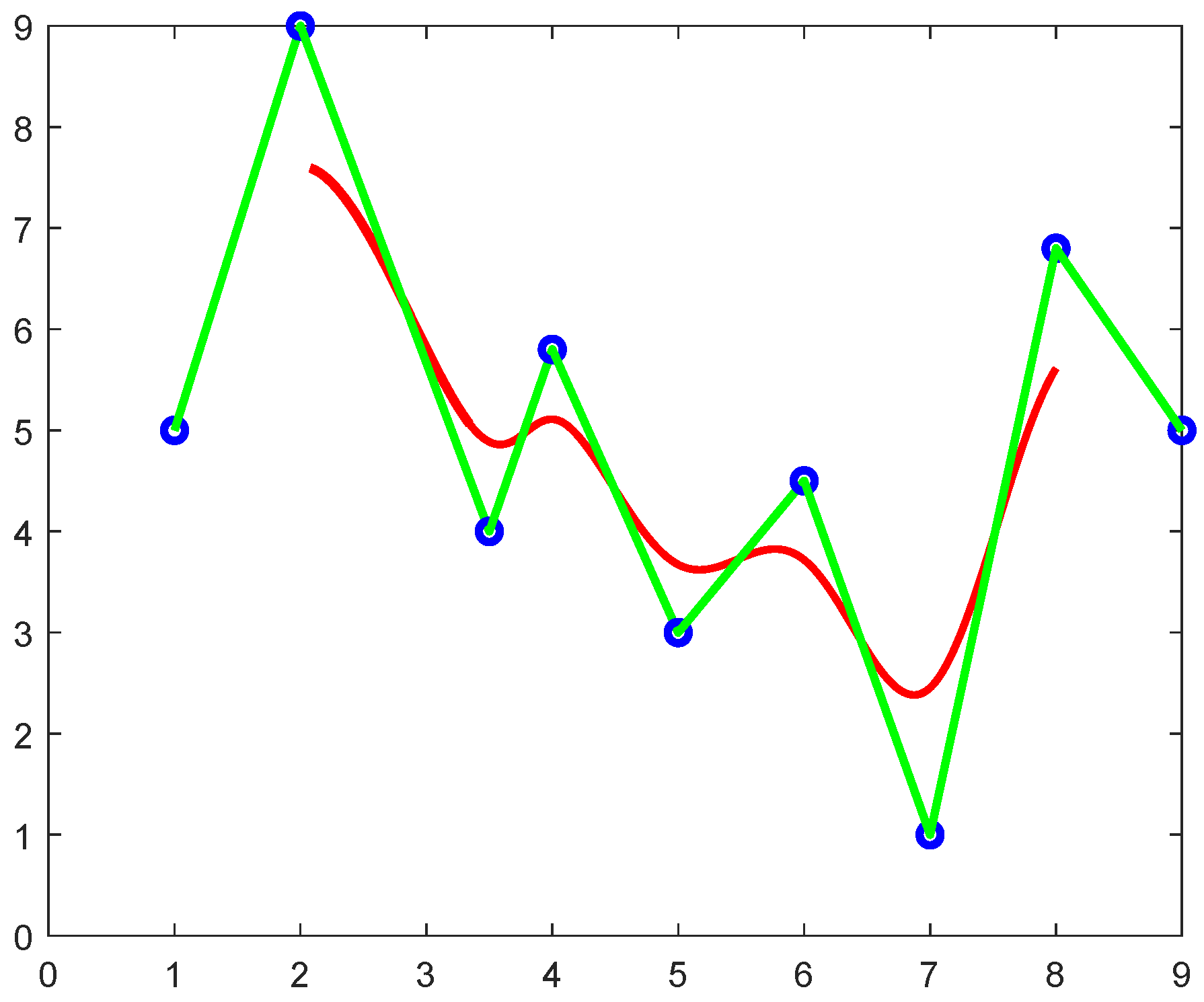
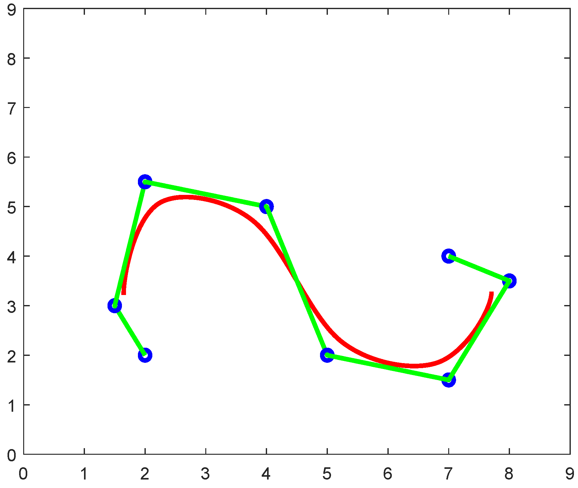
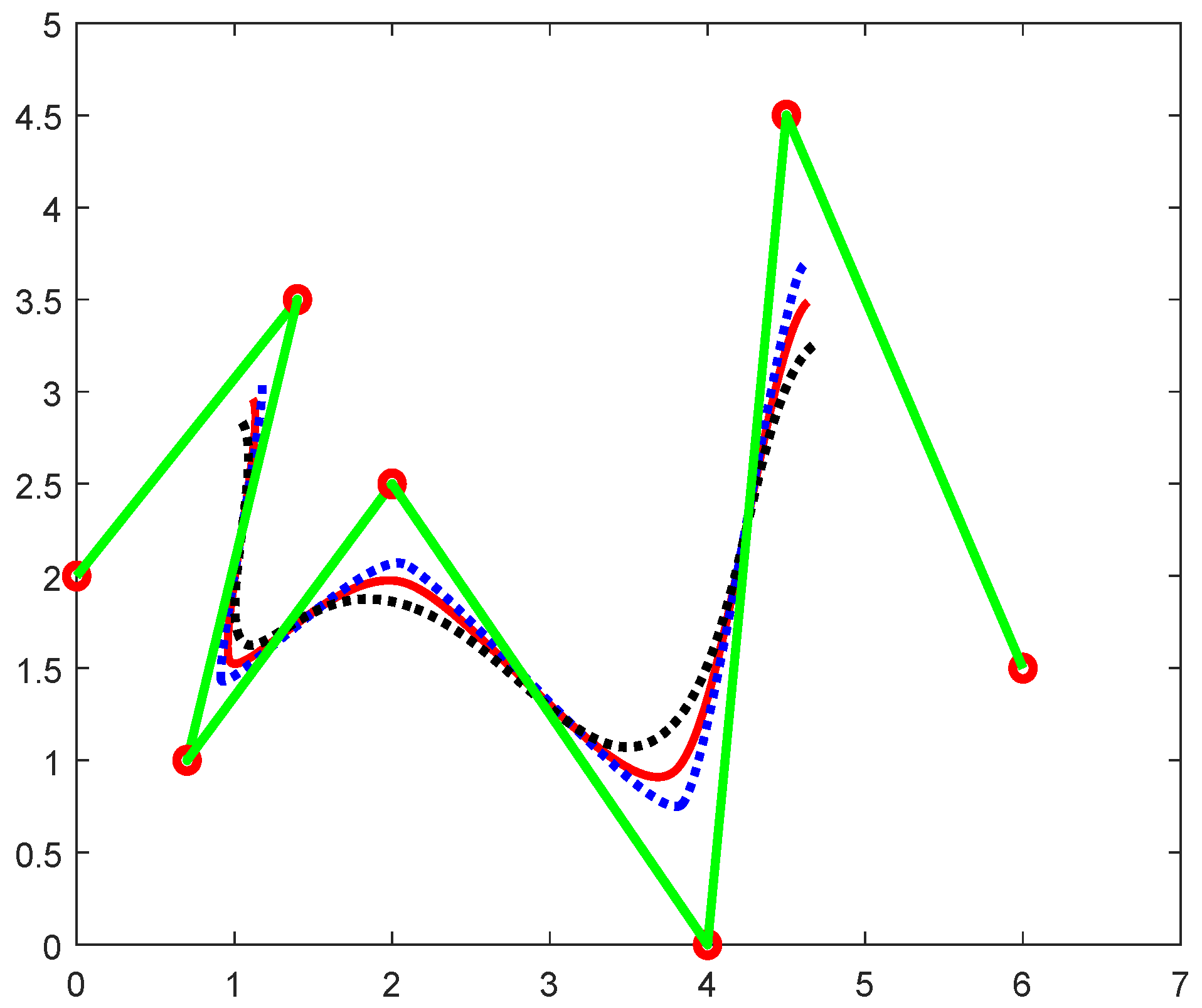
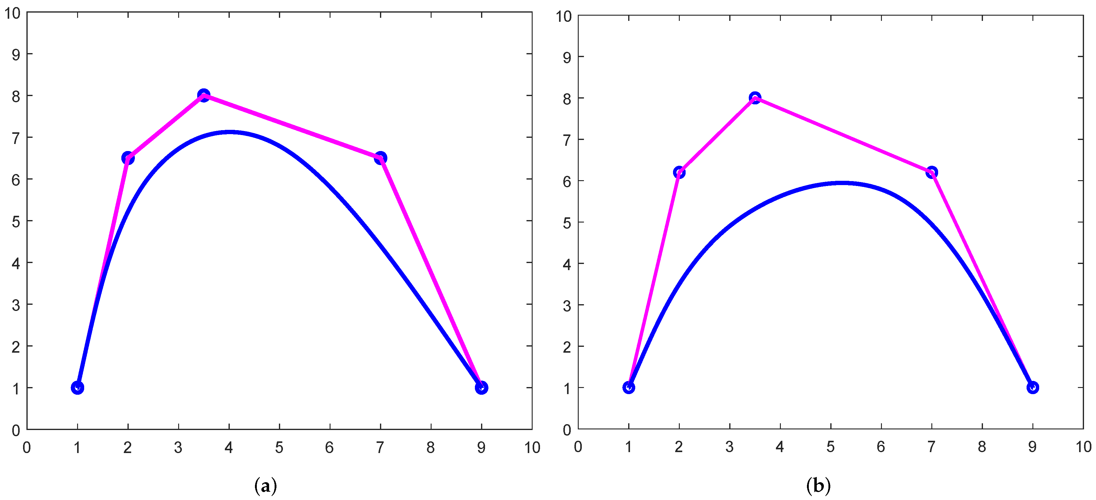
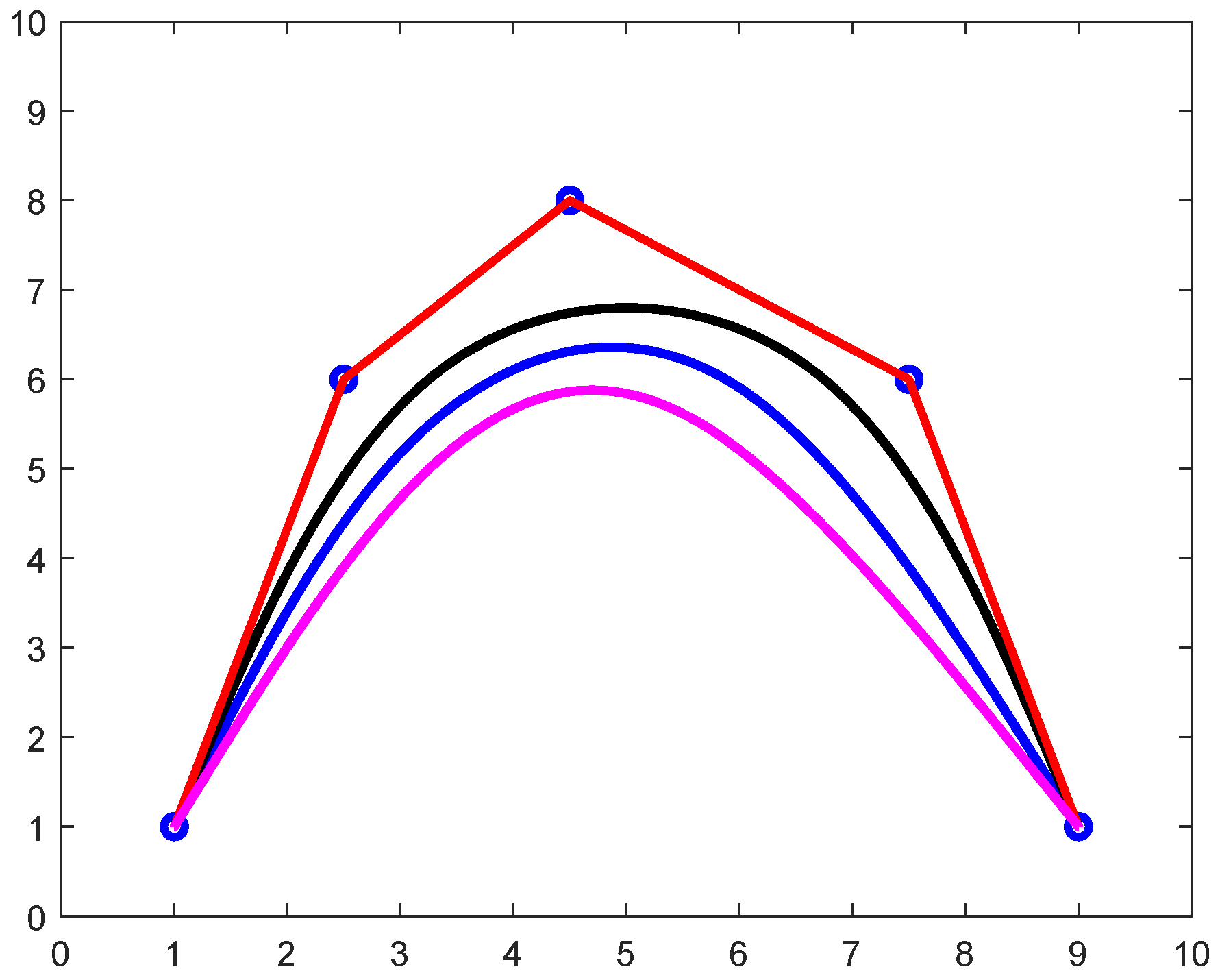
• Open Trigonometric B-spline Curve: The given TBS basis functions are verified by constructing an open B-spline curve by using the SP $\lambda$ and the knot vectors $N=(n_0,n_1,\dots ..,n_{j+4})$. In Figure 9, by taking SP $\lambda =0.2$, an open curve was constructed, and thus it also lies in the convex hull of its defining control polygon.
  The effect of SP is shown in Figure 10 by using different colours. These coloured curves were designed by taking different values of SP, and black is used for $\lambda =0$, red for $\lambda =0.35$ and blue for $\lambda =0.8$.
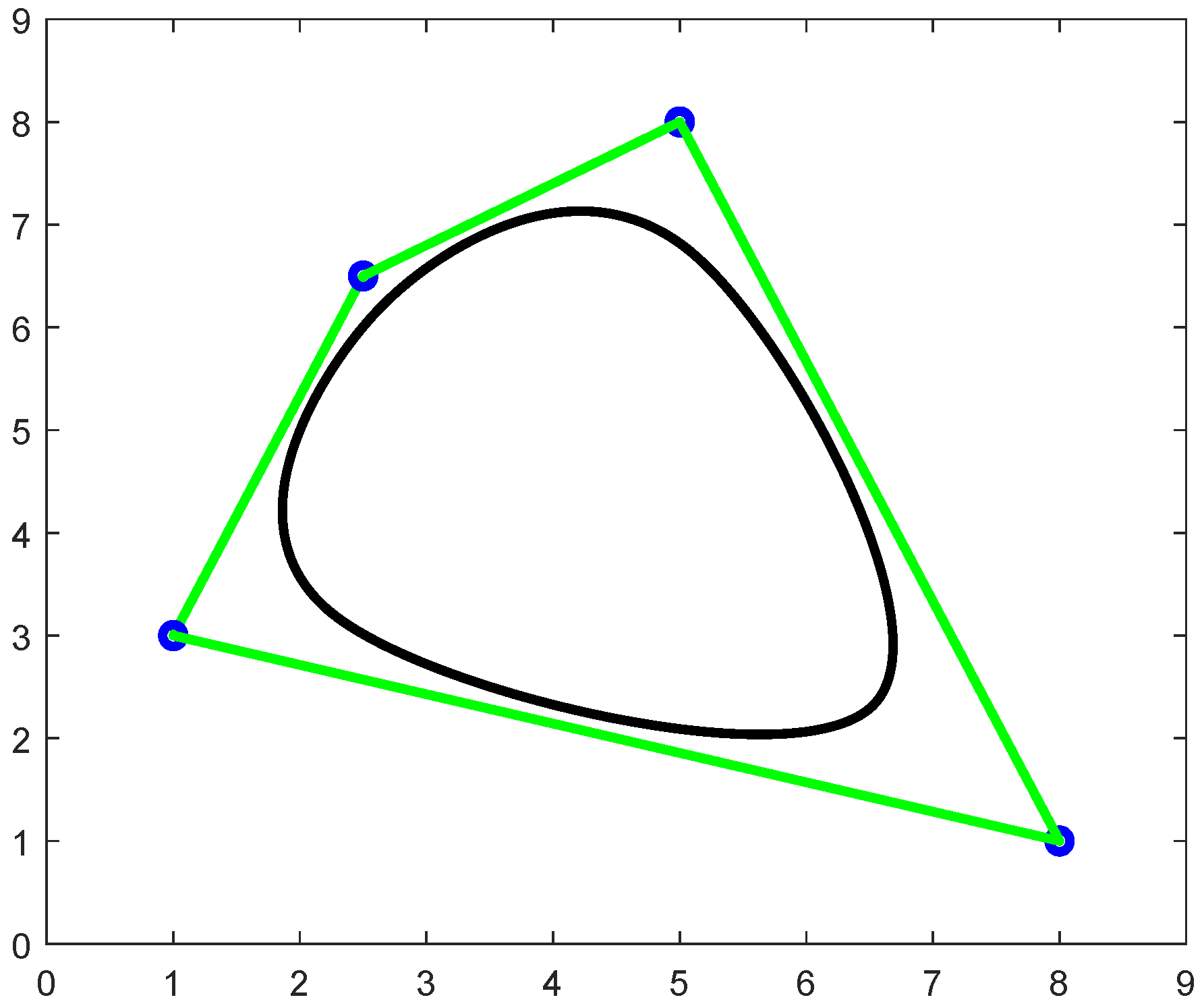
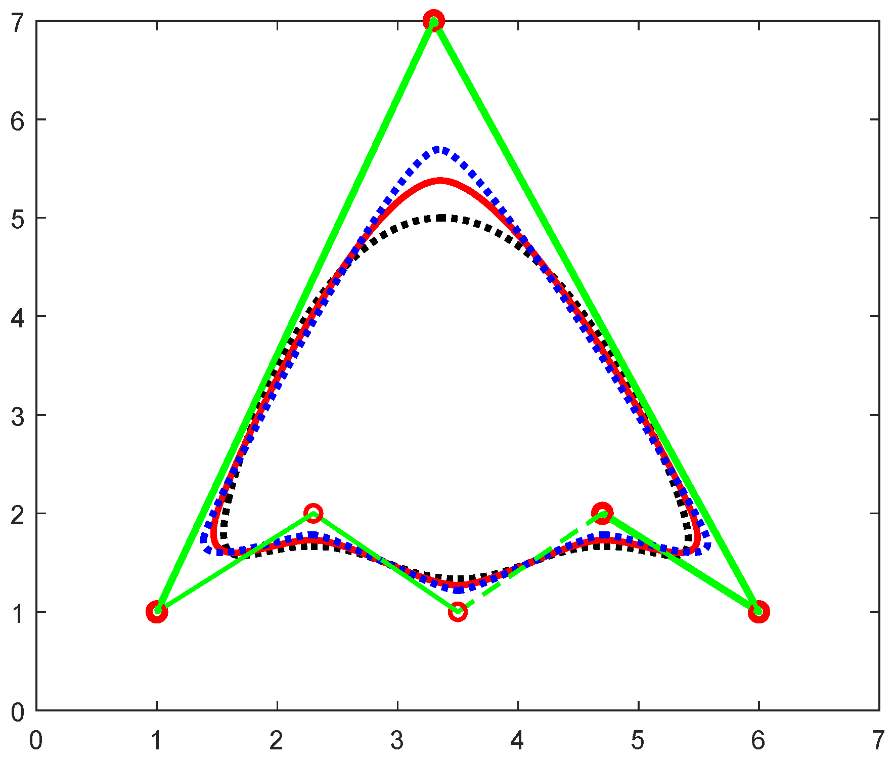
• Closed Trigonometric B-spline Curve: In Figure 11, a closed curve was constructed by using the knot vectors $N=(n_0,n_1,\dots ..,n_{j+4})$ in the interval $n\in [n_i,n_{i+1})$ and specified by using the shape parameter (SP) $\lambda$.
  Therefore, the proposed basis function is applicable for both open and closed cubic TBS curves, and the effect of SP by taking various values of $\lambda$ is shown in Figure 12 with blue used for $\lambda =0.8$, red for $\lambda =0.35$ and black for $\lambda =0$.
  Therefore, it is proven that, by increasing the value of $\lambda$, we obtain more refined forms of curves, which are closer to the control polygon.

4. Cubic Trigonometric Rational B-Spline Basis Functions

Definition 3.

The cubic TRBS basis function with the degree d of the polynomial with the weights $w_i^{\prime }s>0$ is defined as follows.

$$\begin{array}{ccc}\hfill F\left(n\right)& =& \sum _{i=0}^n(\frac{w_i{B}_{i,d}\left(n\right)}{{\sum }_{j=0}^n\left(w_j{B}_{j,d}\left(n\right)\right)}).\hfill \end{array}$$

(6)

Here, $B_{i,d}$ are the cubic TBS basis functions with the knot vectors N.

In addition,

$$\begin{array}{ccc}\hfill F\left(n\right)& =& \sum _{i=0}^n{P}_{i,d}\left(n\right),\hfill \end{array}$$

(7)

where

$$\begin{array}{ccc}\hfill P_{i,d}\left(n\right)& =& (\frac{w_i{B}_{i,d}\left(n\right)}{{\sum }_{j=0}^n\left(w_j{B}_{j,d}\left(n\right)\right)}).\hfill \end{array}$$

Properties of Rational Trigonometric Cubic B-Spline Basis Functions

The following are some of the properties of cubic TRBS basis functions.

Theorem 5.

The sum of all the basis functions of cubic trigonometric rational B-spline (TRBS) is equal to 1, i.e.,

$$\begin{array}{c}\hfill \sum _{i=0}^n{P}_{i,d}\left(n\right)=1.\end{array}$$

Proof. 

Thus,

$$\begin{array}{c}\hfill P_{i,d}\left(n\right)=(\frac{w_i{B}_{i,d}\left(n\right)}{{\sum }_{j=0}^n(w_j{B}_{j,d}\left(n\right))}).\end{array}$$

This can also be written as

$$\begin{array}{c}\hfill P_{i,3}\left(n\right)=(\frac{w_i{B}_{i,3}\left(n\right)}{w_0{B}_{0,3}\left(n\right)+w_1{B}_{1,3}\left(n\right)+w_2{B}_{2,3}\left(n\right)+w_3{B}_{3,3}\left(n\right)}).\end{array}$$

Thus, we have

$$\begin{array}{ccc}\hfill F\left(n\right)& =& \sum _{i=0}^3{P}_{i,3}\left(n\right).\hfill \\ & =& P_{0,3}\left(n\right)+P_{1,3}\left(n\right)+P_{2,3}\left(n\right)+P_{3,3}\left(n\right).\hfill \\ \hfill F\left(n\right)& =& \frac{w_0{B}_{0,3}\left(n\right)}{w_0{B}_{0,3}\left(n\right)+w_1{B}_{1,3}\left(n\right)+w_2{B}_{2,3}\left(n\right)+w_3{B}_{3,3}\left(n\right)}\hfill \\ & & \frac{w_1{B}_{1,3}\left(n\right)}{w_0{B}_{0,3}\left(n\right)+w_1{B}_{1,3}\left(n\right)+w_2{B}_{2,3}\left(n\right)+w_3{B}_{3,3}\left(n\right)}\hfill \\ & & \frac{w_2{B}_{2,3}\left(n\right)}{w_0{B}_{0,3}\left(n\right)+w_1{B}_{1,3}\left(n\right)+w_2{B}_{2,3}\left(n\right)+w_3{B}_{3,3}\left(n\right)}\hfill \\ & & \frac{w_3{B}_{3,3}\left(n\right)}{w_0{B}_{0,3}\left(n\right)+w_1{B}_{1,3}\left(n\right)+w_2{B}_{2,3}\left(n\right)+w_3{B}_{3,3}\left(n\right)}.\hfill \\ \hfill F\left(n\right)& =& \frac{w_0{B}_{0,3}\left(n\right)+w_1{B}_{1,3}\left(n\right)+w_2{B}_{2,3}\left(n\right)+w_3{B}_{3,3}\left(n\right)}{w_0{B}_{0,3}\left(n\right)+w_1{B}_{1,3}\left(n\right)+w_2{B}_{2,3}\left(n\right)+w_3{B}_{3,3}\left(n\right)}.\hfill \\ \hfill F\left(n\right)& =& 1.HenceProved.\hfill \end{array}$$

□

Theorem 6.

For all $w_i=1=w_j$, then $P_{i,d}\left(n\right)=B_{i,d}\left(n\right)$.

Proof. 

The TRBS basis functions for degree $d=3$ is defined as

$$\begin{array}{c}\hfill P_{i,3}\left(n\right)=(\frac{w_i{B}_{i,3}\left(n\right)}{{\sum }_{j=0}^3\left(w_j{B}_{j,3}\left(n\right)\right)}).\end{array}$$

With $w_i=w_j=1$, we find

$$\begin{array}{ccc}\hfill P_{i,3}\left(n\right)& =& (\frac{\left(1\right)B_{i,3}\left(n\right)}{\left(1\right)B_{0,3}\left(n\right)+\left(1\right)B_{1,3}\left(n\right)+\left(1\right)B_{2,3}\left(n\right)+\left(1\right)B_{3,3}\left(n\right)}).\hfill \\ & =& (\frac{B_{i,3}\left(n\right)}{B_{0,3}\left(n\right)+B_{1,3}\left(n\right)+B_{2,3}\left(n\right)+B_{3,3}\left(n\right)}).\hfill \end{array}$$

As we know that the sum of all the basis functions is equal to 1, i.e., this is already proven in the property of the partition of unity. Thus, this implies

$${\sum }_{i=0}^3{B}_i\left(n\right)=1.$$

Therefore, we find

$$P_{i,d}\left(n\right)=B_{i,d}\left(n\right).$$

□

5. Rational Trigonometric Cubic B-Spline Curve

Definition 4.

The Cubic TRBS curve with the free parameter λ and the weights $w_i^{\prime }s>0$ is defined as

$$\begin{array}{ccc}\hfill T\left(n\right)& =& \sum _{i=0}^n(\frac{w_i{K}_i{B}_{i,d}\left(n\right)}{{\sum }_{j=0}^n\left(w_j{B}_{j,d}\left(n\right)\right)}).\hfill \end{array}$$

(8)

where $K_i=K_0,K_1,\dots ,K_m$ are the control points and $B_{i,d}\left(n\right)$ are the trigonometric basis with the degree d at the knot vectors $N=\left(n_0,n_1,\dots ,n_{j+4}\right)$. The above expression can also be written as

$$\begin{array}{c}\hfill F\left(n\right)=(\sum _{i=0}^n{K}_i{P}_{i,d}\left(n\right)),\end{array}$$

(9)

where

$$\begin{array}{c}\\ \hfill P_{i,d}\left(n\right)=(\frac{w_i{B}_{i,d}\left(n\right)}{{\sum }_{j=0}^n\left(w_j{B}_{j,d}\left(n\right)\right)}).\end{array}$$

5.1. Properties of Rational Trigonometric Cubic B-Spline Curve

• Convex Hull Property (CHP): Rational B-spline curve has convex hull property, i.e., every point of curve lies inside the convex hull of its defining polygon. This implies $T\left(n\right)\in CH(K_0,K_1,\dots ,K_m)$ for $n\in [n_i,n_{j+4})$, as shown in Figure 13;
• Local Control:Figure 14 shows that, in B-splines, the curve is always controlled by changing the weights and the control points.
• Invariance Under Affine Transformation: Let T be an affine transformation, and then

  $$\begin{array}{c}\hfill T(\sum _{i=0}^n(\frac{w_i{K}_i{B}_{i,d}\left(n\right)}{{\sum }_{j=0}^n\left(w_j{B}_{j,d}\left(n\right)\right)}))=\sum _{i=0}^n(\frac{w_{i}T\left(K_i\right)B_{i,d}\left(n\right)}{{\sum }_{j=0}^n\left(w_j{B}_{j,d}\left(n\right)\right)}).\end{array}$$
• Continuity of Cubic Rational B-spline Curve: The cubic TRBS curve has $C^1$ continuity at UK vector n. Consider m is the multiplicity of the knot vectors n, which is equal to the order of the cubic B-spline curve, and then the curve has continuity $C^{3-m}$, and $C^{-1}$ continuity implies that the curve is discontinuous.
  For $n\in [n_i,n_{i+1})$, the continuity of the knot vectors is given as

  $$\begin{array}{ccc}\hfill P_{i-3}(n_i^{+})& =& (\frac{w_0}{w_0+4(1+\lambda )w_1+w_2})(K_{i-3}),\hfill \end{array}$$

  (10)

  $$\begin{array}{ccc}\hfill P_{i-2}(n_i^{+})& =& (\frac{4(1+\lambda )(w_1)}{w_0+4(1+\lambda )w_1+w_2})(K_{i-2}),\hfill \end{array}$$

  (11)

  $$\begin{array}{ccc}\hfill P_{i-2}(n_{i+1}^{-})& =& (\frac{w_1}{w_1+4(1+\lambda )w_2+w_3})(K_{i-2}),\hfill \end{array}$$

  (12)

  $$\begin{array}{ccc}\hfill P_{i-1}(n_i^{+})& =& (\frac{w_2}{w_0+4(1+\lambda )w_1+w_2})(K_{i-1}),\hfill \end{array}$$

  (13)

  $$\begin{array}{ccc}\hfill P_{i-1}(n_{i+1}^{-})& =& (\frac{4(1+\lambda )(w_2)}{w_1+4(1+\lambda )w_2+w_3})(K_{i-1}),\hfill \end{array}$$

  (14)

  $$\begin{array}{ccc}\hfill P_i(n_{i+1}^{-})& =& (\frac{w_3}{w_1+4(1+\lambda )w_2+w_3})(K_i).\hfill \end{array}$$

  (15)
  Differentiating Equation (10) w.r.t ‘n’ and then substituting $n=n_i$ in the first derivative of rational curve defined on $n\in [n_i,n_{i+1})$, we obtain

  $$\begin{array}{ccc}\hfill P_{i-3}^{\prime }(n_i^{+})& =& (\frac{\pi }{\Delta n_i})[\frac{(\lambda -2)\{2(1+\lambda )w_1+w_2\}(w_0)}{{(w_0+4(1+\lambda )w_1+w_2)}^2}](K_{i-3}).\hfill \end{array}$$
  Differentiating Equation (11) w.r.t ‘n’ and then substituting $n=n_i$ in the first derivative of rational curve defined on $n\in [n_i,n_{i+1})$, we obtain

  $$\begin{array}{ccc}\hfill P_{i-2}^{\prime }(n_i^{+})& =& (\frac{\pi }{2\Delta n_i})[\frac{(\lambda -2)\left\{4(1+\lambda )(w_0+w_2)\right\}(w_1)}{{(w_0+4(1+\lambda )w_1+w_2)}^2}](K_{i-2}).\hfill \end{array}$$
  Differentiating Equation (12) w.r.t ‘n’ and then substituting $n=n_{i+1}$ in the first derivative of rational curve defined on $n\in [n_i,n_{i+1})$, we obtain

  $$\begin{array}{ccc}\hfill P_{i-2}^{\prime }(n_{i+1}^{-})& =& (\frac{\pi }{2\Delta n_i})[\frac{(\lambda -2)\left\{4(1+\lambda )(w_2+w_3)\right\}(w_1)}{{(w_1+4(1+\lambda )w_2+w_3)}^2}](K_{i-2}).\hfill \end{array}$$
  Differentiating Equation (13) w.r.t ‘n’ and then substituting $n=n_i$ in the first derivative of rational curve defined on $n\in [n_i,n_{i+1})$, we find

  $$\begin{array}{ccc}\hfill P_{i-1}^{\prime }(n_i^{+})& =& (\frac{\pi }{\Delta n_i})[\frac{(2-\lambda )\{(1+\lambda )w_1+w_0\}(w_2)}{{(w_0+4(1+\lambda )w_1+w_2)}^2}](K_{i-1}).\hfill \end{array}$$
  Differentiating Equation (14) w.r.t ‘n’ and then substituting $n=n_{i+1}$ in the first derivative of rational curve defined on $n\in [n_i,n_{i+1})$, we obtain

  $$\begin{array}{ccc}\hfill P_{i-1}^{\prime }(n_{i+1}^{-})& =& (\frac{\pi }{\Delta n_i})[\frac{(2-\lambda )\left\{2(1+\lambda )(w_1-w_3)\right\}(w_2)}{{(w_1+4(1+\lambda )w_2+w_3)}^2}](K_{i-1}).\hfill \end{array}$$
  Differentiating Equation (15) w.r.t ‘n’ and then substituting $n=n_{i+1}$ in the first derivative of rational curve defined on $n\in [n_i,n_{i+1})$, we obtain

  $$\begin{array}{ccc}\hfill P_i^{\prime }(n_{i+1}^{-})& =& (\frac{\pi }{\Delta n_i})[\frac{(2-\lambda )\{w_1+2(1+\lambda )(w_2)\}(w_3)}{{(w_1+4(1+\lambda )w_2+w_3)}^2}](K_i).\hfill \end{array}$$

5.2. Open and Close Trigonometric Rational B-Spline Curve

• Open Rational B-Spline Curve: An open TRBS curve can be constructed by using control point multiplicity as shown in Figure 15 and obtain an end point interpolated curve.
• Close Rational B-spline Curve: By using the uniform knots (UK), we can construct closed or periodic cubic trigonometric rational B-spline (TRBS) curve as shown in Figure 16. The curve in blue colour is constructed by taking $\lambda =0.65$. Black colour shows the value of SP $\lambda$ as $\lambda =0.3$. Whereas for $\lambda =0.1$ we use red colour. The effect of shape parameter (SP) is observed in the figure below and

  Table 2. Different values of weights for open and closed rational curves.

  value of $w_0$	9	19	17
  value of $w_1$	7	10	5
  value of $w_2$	8	18	12
  value of $w_3$	7	27	47

  shows the effect of weights.

6. Applications

The proposed scheme was used for the construction of open and closed curves and to design different shapes, such as alphabet, star, butterfly and leaf with the suitable choice of SPs and weights.

• Alphabet Designing: Twelve control points are used for the designing of an alphabet M. Thus it is seen that by change the value of SP, we obtain a more refined shape of the letter M. In Figure 17a firstly we take $\lambda =0$ and then in Figure 17b we take $\lambda =0.8$. As we increase the value of SP we see that an alphabet become more finer.
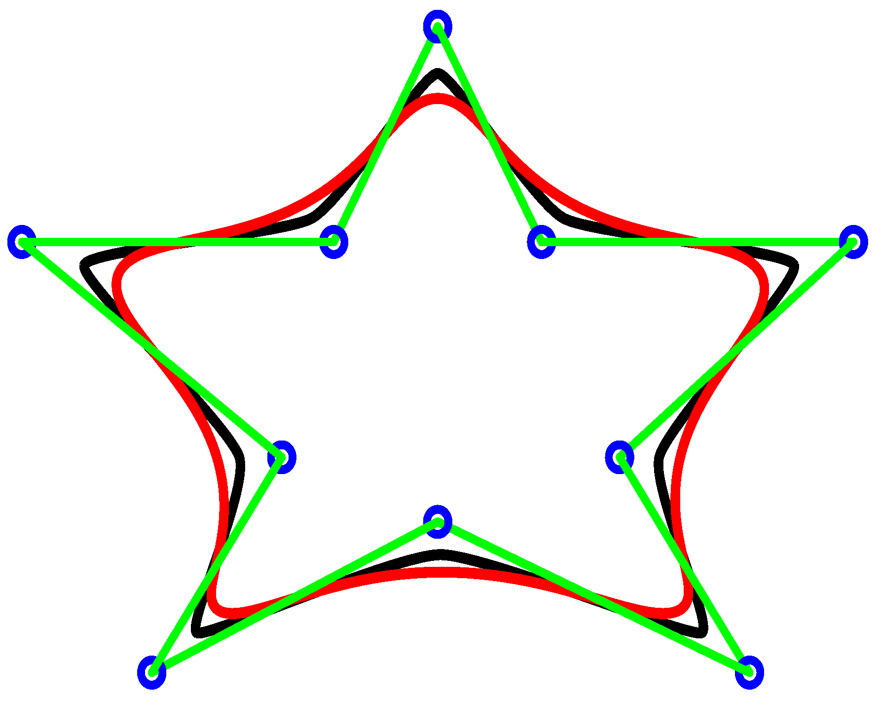
• Star Designing: The cubic trigonometric rational B-spline (TRBS) curve is used in the designing of star by taking 10 control points. In the star construction, the SP $\lambda =0.8$ is used in black colour. Whereas $\lambda =0$ in red colour indicates the effect of SP and weights as seen in Figure 18.
• Butterfly design: A butterfly was constructed by using a cubic TBS curve as shown in Figure 19. A total of 92 control points are used in the construction of butterfly. By using different values of SP, such as at $\lambda =0.5$, the wings of the butterfly are designed. furthermore, for $\lambda =0.1$ the remaining part of the butterfly was designed. The adjustment in the value of SP works efficiently and gives a finer object.
• 3D cube construction: A geometrical model of a cube in a 3-dimensional manner was designed in the figure below by using cubic TRBs curve. The free parameter $\lambda =0.1$ was used in this model. Different colour curves are used to represent the effect of control points. Thus, it was seen that all the curves lies inside its defining polygon as shown in Figure 20.
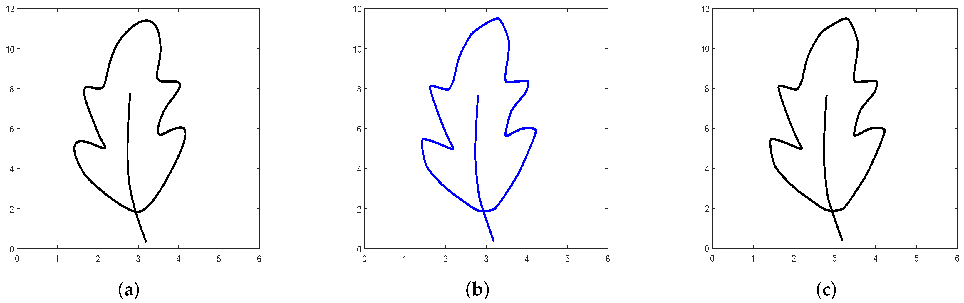
• Leaf Design: Trigonometric B-spline curve was used to create a geometrical design of a leaf. The model of leaf in Figure 21a was formed by using the value of SP $\lambda =0$. Then we take $\lambda =0.35$ in Figure 21b to construct the geometrical design of a leaf whereas in Figure 21c we take the value of SP at $\lambda =0.6$.
  Therefore, we see that the shape of the leaf becomes finer as the value of the SP is raised.

7. Conclusions

In this paper, we presented cubic TBS curves in both polynomial and rational forms. Both of the curves satisfied all the basis properties, such as the partition of unity and positivity. The continuity of the proposed scheme was also checked but using the defined basis functions. The flexibility of the preserved basis was also checked by constructing different models—for example, alphabet design, butterfly construction and making a leaf, a star and a model of a cube in $3D$ by using appropriate values of the SP and weights. Hence, we conclude that TBS curves are more beneficial than trigonometric Bézier curves. In the future, the surface can be constructed by using the proposed basis. The applicability of the basis functions can be improved by taking more shape parameters and by extending the interval of SPs.

References

1. Farin, G.E.; Josef, H.; Myung-Soo, K. Handbook of Computer Aided Geometric Design; Elsevier: Boston, MA, USA; London, UK; New York, NY, USA, 2002. [Google Scholar]
2. Farin, G.E. Curves and Surfaces for Computer-Aided Geometric Design: A Practical Code; Academic Press Inc.: Cambridge, MA, USA, 1996. [Google Scholar]
3. Majeed, A.; Abbas, M.; Miura, K.T.; Kamran, M.; Nazir, T. Surface modeling from 2D contours with an application to craniofacial fracture construction. Mathematics 2020, 8, 1246. [Google Scholar] [CrossRef]
4. Li, F.; Hu, G.; Abbas, M.; Miura, K.T. The generalized H-Bézier model: Geometric continuity conditions and applications to curve and surface modeling. Mathematics 2020, 8, 924. [Google Scholar] [CrossRef]
5. Hu, X.; Hu, G.; Abbas, M.; Misro, M.Y. Approximate multi-degree reduction of Q-Bézie curves via generalized Bernstein polynomial functions. Adv. Differ. Equ. 2020, 2020, 413. [Google Scholar] [CrossRef]
6. Sánchez-Reyes, J. Harmonic rational Bézier curves, p-Bézier curves and trigonometric polynomials. Comput. Aided Geom. Des. 1998, 15, 909–923. [Google Scholar] [CrossRef]
7. González, C.; Albrecht, G.; Paluszny, M.; Lentini, M. Design of C2 algebraic-trigonometric pythagorean hodograph splines with shape parameters. Comput. Appl. Math. 2018, 37, 1472–1495. [Google Scholar]
8. Pelosi, F.; Farouki, R.T.; Manni, C.; Sestini, A. Geometric Hermite interpolation by spatial Pythagorean-hodograph cubics. Adv. Comput. Math. 2005, 22, 325–352. [Google Scholar] [CrossRef]
9. Zhu, Y.; Han, X. New trigonometric basis possessing exponential shape parameters. J. Comput. Math. 2015, 33, 642–684. [Google Scholar]
10. Levent, A.; Sahin, B. Cubic Bézier-like transition curves with new basis function. Proc. Inst. Math. Mech. Natl. Acad. Sci. Azerbaijan 2018, 44, 222–228. [Google Scholar]
11. Han, X.A.; Ma, Y.; Huang, X. The cubic trigonometric Bézier curve with two shape parameters. Appl. Math. Lett. 2009, 22, 226–231. [Google Scholar] [CrossRef] [Green Version]
12. Troll, E. Constrained modification of the cubic trigonometric Bézier curve with two shape parameters. Ann. Math. Inform. 2014, 43, 145–156. [Google Scholar]
13. Chen, Q.; Wang, G. A class of Bézier-like curves. Comput. Aided Geom. Des. 2003, 20, 29–39. [Google Scholar] [CrossRef]
14. Chen, X.; Tan, J.; Liu, Z.; Xie, J. Approximation of functions by a new family of generalized Bernstein operators. J. Math. Anal. Appl. 2017, 450, 244–261. [Google Scholar] [CrossRef]
15. Oruç, H.; Phillips, G.M. q-Bernstein polynomials and Bézier curves. J. Comput. Appl. Math. 2003, 151, 1–12. [Google Scholar] [CrossRef] [Green Version]
16. Ait-Haddou, R.; Barton, M. Constrained multi-degree reduction with respect to Jacobi norms. Comput. Aided Geom. Des. 2016, 42, 23–30. [Google Scholar] [CrossRef] [Green Version]
17. Srivastava, H.M.; Ansari, K.J.; Ozger, F.; OdemisOzger, Z. A link between approximation theory and summability methods via four-dimensional infinite matrices. Mathematics 2021, 9, 1895. [Google Scholar] [CrossRef]
18. Schoenberg, I.J. On trigonometric spline interpolation. J. Math. Mech. 1964, 13, 795–825. [Google Scholar]
19. Troll, E.M.; Hoffmann, M. Geometric properties and constrained modification of trigonometric spline curves of Han. Ann. Math. Inform. 2010, 37, 165–175. [Google Scholar]
20. Dung, V.T.; Tjahjowidodo, T. A direct method to solve optimal knots of B-spline curves: An application for non-uniform B-spline curves fitting. PLoS ONE 2017, 12, e0173857. [Google Scholar] [CrossRef]
21. Han, X. Quadratic trigonometric polynomial curves with a shape parameter. Comput. Aided Geom. Des. 2002, 19, 503–512. [Google Scholar] [CrossRef]
22. Piegl, L.; Tiller, W. The NURBS Book; Springer: New York, NY, USA, 1995. [Google Scholar]
23. Marsh, D. Applied Geometry for Computer Graphics and CAD; Springer Science & Business Media: Berlin/Heidelberg, Germany, 2005. [Google Scholar]
24. Choubey, N.; Ojha, A. Trigonometric splines with variable shape parameter. Rocky Mt. J. Math. 2008, 38, 91–105. [Google Scholar] [CrossRef]
25. Han, X. Cubic trigonometric polynomial curves with a shape parameter. Comput. Aided Geom. Des. 2004, 21, 535–548. [Google Scholar] [CrossRef]
26. Yan, L. Cubic trigonometric nonuniform spline curves and surfaces. Math. Probl. Eng. 2016, 2016, 7067408. [Google Scholar] [CrossRef] [Green Version]
27. Yan, L.; Liang, J. A class of algebraic–trigonometric blended splines. J. Comput. Appl. Math. 2011, 235, 1713–1729. [Google Scholar] [CrossRef]
28. Hu, G.; Qin, X.; Ji, X.; Wei, G.; Zhang, S. The construction of μ-B-spline curves and its application to rotational surfaces. Appl. Math. Comput. 2015, 266, 194–211. [Google Scholar] [CrossRef]
29. Majeed, A.; Qayyum, F. New rational cubic trigonometric B-spline curves with two shape parameters. Comput. Appl. Math. 2020, 39, 198. [Google Scholar] [CrossRef]
30. Pagani, L.; Scott, P.J. Curvature based sampling of curves and surfaces. Comput. Aided Geom. Des. 2018, 59, 32–48. [Google Scholar] [CrossRef]
31. Walz, G. Identities for trigonometric B-splines with an application to curve design. BIT Numer. Math. 1997, 37, 189–201. [Google Scholar] [CrossRef]
32. Majeed, A.; Mt Piah, A.R.; Gobithaasan, R.U.; Yahya, Z.R. Craniofacial reconstruction using rational cubic ball curves. PLoS ONE 2015, 10, e0122854. [Google Scholar] [CrossRef]
33. Majeed, A.; Rafique, M.; Abdullah, J.Y.; Rajion, Z.A. NURBS curves with the application of multiple bones fracture reconstruction. Appl. Math. Comput. 2017, 315, 70–84. [Google Scholar] [CrossRef]
Figure 1. Cubic TBFs curves. (a) λ [ 0 , 8 ) , (b) λ [ 2 , 10 ) , (c) λ [ 4 , 12 ) and (d) λ [ 6 , 14 ) .
Mathematics 10 01087 g001
Figure 2. Cubic TBS basis functions at [ 0 , 14 ) .
Mathematics 10 01087 g002
Figure 3. Effect of SP.
Mathematics 10 01087 g003
Figure 4. Symmetry of CTBS functions. (a) Symmetry of the first function. (b) Symmetry of the fourth function. (c) Symmetry of the second function. (d) Symmetry of the third function.
Mathematics 10 01087 g004
Figure 5. Plot of the second derivative of the basis function.
Mathematics 10 01087 g005
Figure 6. Cubic trigonometric B-spline curve.
Mathematics 10 01087 g006
Figure 7. Local control property.
Mathematics 10 01087 g007
Figure 8. Convex hull property of the cubic TBS curve.
Mathematics 10 01087 g008
Figure 9. Open curve using CTBS basis functions.
Mathematics 10 01087 g009
Figure 10. Effect of SP on an open B-spline curve.
Mathematics 10 01087 g010
Figure 11. Closed curve using CTBS basis functions.
Mathematics 10 01087 g011
Figure 12. Effect of SP.
Mathematics 10 01087 g012
Figure 13. Convex hull property of a rational curve.
Mathematics 10 01087 g013
Figure 14. Cubic rational B-spline curve. (a) Effect of control points. (b) Effect of weights.
Mathematics 10 01087 g014
Figure 15. Open rational B-spline curve.
Mathematics 10 01087 g015
Figure 16. Closed TRBS curve with different weights.
Mathematics 10 01087 g016
Figure 17. Designing an alphabet.
Mathematics 10 01087 g017
Figure 18. Star designing using rational B-spline curves.
Mathematics 10 01087 g018
Figure 19. Butterfly designing using rational B-spline function.
Mathematics 10 01087 g019
Figure 20. 3D cube construction using TRBS.
Mathematics 10 01087 g020
Figure 21. Leaf designing using cubic trigonometric B-spline curves. (a) Leaf designing at λ = 0 . (b) Leaf designing λ = 0.35 . (c) Leaf designing λ = 0.6 .
Mathematics 10 01087 g021