Rigorous Analysis of the Quasi-Steady-State Assumption in Enzyme Kinetics

Abstract

We study, from a purely quantitative point of view, the quasi-steady-state assumption for the fundamental mathematical model of the general enzymatic reaction. In particular, $\left(\mathrm{i}\right)$ we introduce a simple, yet generic, algorithm for the proper scaling of the corresponding problem, $\left(\mathrm{ii}\right)$ we define the two essential parts (the standard and the reverse) of the quasi-steady-state assumption in a quantitative fashion, and $\left(\mathrm{iii}\right)$ we comment on the dispensable, although widely adopted, third part (the total) of it.

1. Introduction

The study of the fundamental mathematical model for the kinetics of the general enzymatic reaction with chemical equation

$$S+E\to E+P,$$

(1)

where S is the substrate, P is the product and E is the enzyme that catalyzes it, has a long history, which we briefly present below.

In 1894, Fischer [1] derived the lock and key model for the interpretation of biocatalysis. Before 1901, Brown suggested an intermediate step in the enzymatic reaction that was described by (1), where the substrate forms a complex with the enzyme before the beginning of the catalysis, an idea that was eventually published in 1902 [2]. Thus, it had already been realized by that time, that enzymatic biochemical reactions take place in at least two stages, and in fact these stages have different time scales. Based on this idea, combined with conversations he had with Bodenstein, Henri published in 1902 [3] and then in 1903 [4] an initial version of a reliable differential equation for the description of the kinetics of the enzyme reaction with the chemical equation given by (1), an idea he had conceived as early as 1901. A decade later, in 1913, Michaelis and Menten [5] (translated in English in [6]) extracted this equation by using a more detailed and analytical form that made use of the rapid equilibrium assumption; they interpreted it convincingly and studied it thoroughly. In particular, using as an example the invertase-catalyzed hydrolysis of sucrose into glucose and fructose, they studied (1) through the chemical mechanism

$$S+E\underset{k_{-1}}{\stackrel{k_1}{\rightleftharpoons }}C\stackrel{k_2}{\to }E+P,$$

(2)

where $k_1,k_{-1},k_2>0$ and C represents the substrate-enzyme complex, and indirectly concluded that, when

$$\left[S\right]={\left[S\right]}_0\gg {\left[E\right]}_0=\left[E\right] \mathrm{and} \left[C\right]={\left[C\right]}_0=0, \mathrm{for} t=0,$$

(3)

a condition acceptable in enzymatic reactions, then for the rate $\upsilon$ of the enzymatic reaction with chemical Equation (1) it holds that

$$\upsilon \approx \frac{{\upsilon }_{sup}\left[S\right]}{K_{\mathrm{dis}}+\left[S\right]},$$

(4)

where

$${\upsilon }_{sup}:=k_2{\left[E\right]}_0,$$

and

$$K_{\mathrm{dis}}:=\frac{k_{-1}}{k_1}.$$

(5)

$K_{\mathrm{dis}}$ is the constant that is nowadays called the dissociation constant (of the complex).

In contrast, Van Slyke and Cullen, working in parallel with Michaelis and Menten, but studying urease-catalyzed hydrolysis of urea to ammonia and carbon dioxide, used—instead of (2)—the chemical mechanism

$$S+E\stackrel{k_1}{\to }C\stackrel{k_2}{\to }E+P$$

and concluded in 1914 [7] to

$$\upsilon \approx \frac{{\upsilon }_{sup}\left[S\right]}{K_{VSC}+\left[S\right]},$$

(6)

instead of (4), where

$$K_{VSC}:=\frac{k_2}{k_1}.$$

(7)

$K_{VSC}$ is a constant that is now known as the Van Slyke–Cullen constant.

In 1925, Briggs and Haldane [8] published a short note where they composed the ideas of Michaelis & Menten and Van Slyke & Cullen through a raw first version of a new enzyme kinetics assumption (already used for chemical kinetics in 1913), known presently as the standard quasi-steady-state assumption. In particular, they improved (4) and (6), demonstrating that:

$$\upsilon \approx \frac{{\upsilon }_{sup}\left[S\right]}{K_M+\left[S\right]},$$

(8)

where:

$$K_M:=K_{\mathrm{dis}}+K_{VSC}=\frac{k_{-1}+k_2}{k_1}.$$

(9)

It is a standard expression nowadays, that “(8) characterizes the Michaelis–Menten kinetics”, and the constant (9) is called the Michaelis–Menten constant.

Lineweaver and Burk in 1934 [9] established (8) in the form:

$$\frac{1}{\upsilon }\approx \frac{1}{{\upsilon }_{sup}}+\frac{K_M}{{\upsilon }_{sup}}\frac{1}{\left[S\right]},$$

as a tool for experimental calculation of the values ${\upsilon }_{sup}$ and $K_M$.

Already since the beginning of the second half of the 20th century and throughout it, many researchers have dealt with the validity of the quasi-steady-state assumption and the determination of the two time scales of the model through the application of perturbation methods. However, it was much later, in 1988 and in 1989, when Segel [10], and Segel and Slemrod [11], respectively, showed that if:

$$\left(K_M+{\left[S\right]}_0\right)\gg {\left[E\right]}_0 \mathrm{and} {\left[C\right]}_0=0,$$

(10)

then there are indeed two time scales, which are recorded as follows:

$$t_C=\frac{1}{k_1\left(K_M+{\left[S\right]}_0\right)}\ll \frac{K_M+{\left[S\right]}_0}{k_2{\left[E\right]}_0}=t_S,$$

and it holds that:

$$\upsilon \approx \left\{\begin{array}{cc}0,\hfill & \mathrm{for} \mathrm{times} \mathrm{comparable} \mathrm{to} t_C,\hfill \\ \mathrm{as} \mathrm{in} \left(8\right),\hfill & \mathrm{for} \mathrm{times} \mathrm{comparable} \mathrm{to} t_S.\hfill \end{array}\right.$$

(11)

In fact, (10) is more general than (3) since it allows:

$$\frac{{\left[E\right]}_0}{{\left[S\right]}_0}=O\left(1\right), \mathrm{as} \frac{{\left[E\right]}_0}{K_M+{\left[S\right]}_0}\to 0^{+},$$

or even:

$${\left[E\right]}_0\gg {\left[S\right]}_0.$$

In 1997, Schnell and Mendoza [12] captured the solution of the Michaelis–Menten kinetics equation in closed form, by using the Lambert W function, and in particular a special case of it, which is defined by its inverse as follows:

$$W^{-1}\left(x\right)=xexp\left\{x\right\}, \forall x\ge 0.$$

In addition, via the aforementioned work of Segel and Slemrod, an initial form of another hypothesis was introduced for the first time, the reverse quasi-steady-state assumption, and it was shown that, when:

$${\left[E\right]}_0\gg K_M \mathrm{and} {\left[C\right]}_0=0,$$

(12)

then there are again two time scales:

$${\tilde{t}}_S=\frac{1}{k_1{\left[E\right]}_0}\ll \frac{1}{k_2}={\tilde{t}}_C,$$

and it holds that:

$$\upsilon \approx \left\{\begin{array}{cc}{k}_1{\left[E\right]}_0\left[S\right],\hfill & \mathrm{for} \mathrm{times} \mathrm{comparable} \mathrm{to} {\tilde{t}}_S,\hfill \\ 0,\hfill & \mathrm{for} \mathrm{times} \mathrm{comparable} \mathrm{to} {\tilde{t}}_C.\hfill \end{array}\right.$$

(13)

About a decade later, in 2000, Schnell and Maini [13] found that (12) is not sufficient for (13) to hold; on the contrary, the new case should have the form:

$${\left[E\right]}_0\gg K_M, {\left[E\right]}_0\gg {\left[S\right]}_0 \mathrm{and} {\left[C\right]}_0=0.$$

(14)

Finally, let us mention that in 1996, with the work of Borghans, Boer and Segel [14], the total substrate concentration, $\left[T\right]$ is introduced, i.e., the sum of the concentration of the unbound/free substrate plus the concentration of the bound substrate in the form of complex with the enzyme, that is:

$$\left[T\right]:=\left[S\right]+\left[C\right],$$

(15)

to describe an alleged third hypothesis that shares common ground with both the previous ones, the so-called total quasi-steady-state assumption, and since then several researchers have adopted and dealt with this hypothesis.

In this work, our novel results are:

• We propose a general and simple algorithm for the proper scaling of every problem with non negative solutions in a bounded domain, and we employ it, in an essential way, for the problem considered in the present paper. Until now, only a “rough” rule for the non dimensionalisation process is utilised in applications, which states that the scales considered for the variables of a problem are chosen so that they should be roughly of the same order of magnitude of the respective variables themselves [15]. The proposed procedure is described by the algorithm with the following steps:

  $$\begin{array}{cc}\begin{array}{ll}{\mathfrak{A}}_1.& \mathit{Identification}\mathit{of}\mathit{the}\mathit{bounded}\mathit{feasible}\mathit{region}—\mathit{i}.\mathit{e}.,\mathit{the}\mathit{range}\mathit{of}\mathit{the}\mathit{dependent}\\ & \mathit{variables}—\mathit{of}\mathit{the}\mathit{problem}.& \\ {\mathfrak{A}}_2.& \mathit{Scaling}\mathit{of}\mathit{the}\mathit{dependent}\mathit{variables}\mathit{of}\mathit{the}\mathit{problem}\mathit{by}\mathit{their}\mathit{respective}\mathit{supremum}\\ & \mathit{feasible}\mathit{values}—\mathit{which}\mathit{do}\mathit{exist},\mathit{since}\mathit{the}\mathit{nonnegative}\mathit{solutions}\mathit{exist}\mathit{in}\mathit{a}& \\ & \mathit{bounded}\mathit{domain}.& \\ {\mathfrak{A}}_3.& \mathit{Natural}\mathit{scaling}\mathit{of}\mathit{the}\mathit{independent}\mathit{variables}\mathit{by}\mathit{gathering}\mathit{the}\mathit{remaining}& \\ & \mathit{terms}\mathit{of}\mathit{the}\mathit{previous}\mathit{step}.& \end{array}& \mathfrak{A}\end{array}$$

• By this algorithm,

  ∘

  the dependent variables are asymptotically comparable with each other, since they all range onto $\left[0,1\right]$,

  ∘

  any scale of the independent variables follows naturally by the process, hence there is no need of the unjustified approach of considering “an estimate of the minimum value for which the variable undergoes a significant change in magnitude” (see, e.g., [10,11,16], which is widely adopted thenceforth), for the choice of the largest of the two time scales appearing in the present problem,

  ∘

  the quantity $\epsilon$, that characterizes both the standard and the reverse quasi-steady-state assumptions, arises effortlessly from the problem itself.

2

We clarify the fully justified, purely quantitative nature of the standard and the reverse quasi-steady-state assumptions. In particular, (sQSSA) and (rQSSA) do not serve for the validation of the standard and the reverse, respectively, quasi-steady-state assumptions—as it is done in [10,11] and all their successors—but they define them.

3

We relinquish the, so-called, total quasi-steady-state assumption, by showing that, in fact, there is no substantive third hypothesis, but only a different approach to the first two (We note that such a duality, characterized by a positive parameter $\epsilon$, that either tends to 0 or to ∞, is common in applications, for instance in the study of Hamiltonian systems possessing either a relatively small or a relatively large Hamiltonian.).

For the sake of brevity, we neither state nor discuss the necessary concepts and fundamental results on solutions of Cauchy problems for vector first order ODEs, such as: $\left(\mathrm{i}\right)$ Existence, uniqueness, extendability, regularity, continuous and smooth dependence on data, local and global stability. There is a huge literature on these topics; indicatively, we refer to [17,18,19,20]. $\left(\mathrm{ii}\right)$ Process of matching, where approximate solutions, accurate in one region of the problem domain, are matched to different approximate solutions, accurate in another region. This subject is discussed in many books, see, e.g., [15,16,21,22]. Although we utilize methods of asymptotic analysis, no singular perturbation expansions are used in the present paper.

2. Principal Analysis of the Problem

In this section, we introduce the main problem and proceed to its basic analysis that comprises the identification of the feasible regions, the well posedness of the problem, the determination of the invariant sets and the simplification and stability analysis of the problem.

2.1. Cauchy Problem

Employing the chemical mechanism (2) along with the Law of Mass Action [23], we arrive at the equations:

$$\begin{array}{cc}\hfill {\displaystyle \frac{\mathrm{d}\left[S\right]}{\mathrm{d}t}}& =-k_1\left[S\right]\left[E\right]+k_{-1}\left[C\right],\hfill \end{array}$$

(16a)

$$\begin{array}{cc}\hfill {\displaystyle \frac{\mathrm{d}\left[E\right]}{\mathrm{d}t}}& =-k_1\left[S\right]\left[E\right]+\left(k_{-1}+k_2\right)\left[C\right],\hfill \end{array}$$

(16b)

$$\begin{array}{cc}\hfill {\displaystyle \frac{\mathrm{d}\left[C\right]}{\mathrm{d}t}}& =k_1\left[S\right]\left[E\right]-\left(k_{-1}+k_2\right)\left[C\right],\hfill \end{array}$$

(16c)

$$\begin{array}{cc}\hfill {\displaystyle \frac{\mathrm{d}\left[P\right]}{\mathrm{d}t}}& =k_2\left[C\right],\hfill \end{array}$$

(16d)

and the corresponding Cauchy problem reads:

$$\begin{array}{c}\mathit{Given} {\left[\mathit{S}\right]}_0,{\left[\mathit{E}\right]}_0,{\left[\mathit{C}\right]}_0,{\left[\mathit{P}\right]}_0\ge 0, \mathit{we} \mathit{seek} \mathit{an} \mathit{interval} \mathcal{I}\subseteq \mathbb{R} \mathit{with} 0\in \mathcal{I}, \mathit{and} \mathit{a}\\ \mathit{function} \left(\left[\mathit{S}\right],\left[\mathit{E}\right],\left[\mathit{C}\right],\left[\mathit{P}\right]\right):\mathcal{I}\to {\left[0,\infty \right)}^4, \mathit{such} \mathit{that} \left(\left[\mathit{S}\right],\left[\mathit{E}\right],\left[\mathit{C}\right],\left[\mathit{P}\right]\right)\\ \mathit{satisfies} \mathit{both} \left(16\right)\mathit{in} {\left(\mathcal{I}\setminus \left\{0\right\}\right)}^{\circ } \mathit{and}\\ \left(\left[\mathit{S}\right],\left[\mathit{E}\right],\left[\mathit{C}\right],\left[\mathit{P}\right]\right)=\left({\left[\mathit{S}\right]}_0,{\left[\mathit{E}\right]}_0,{\left[\mathit{C}\right]}_0,{\left[\mathit{P}\right]}_0\right), \mathit{for} \mathit{t}=0.\end{array}$$

(SECP)

For a solution of (SECP) it holds that:

$${\displaystyle \frac{\mathrm{d}\left[S\right]}{\mathrm{d}t}}+{\displaystyle \frac{\mathrm{d}\left[C\right]}{\mathrm{d}t}}+{\displaystyle \frac{\mathrm{d}\left[P\right]}{\mathrm{d}t}}=0,$$

or, equivalently,

$$\left[S\right]+\left[C\right]+\left[P\right]={\left[S\right]}_0+{\left[C\right]}_0+{\left[P\right]}_0=:A_1,$$

(17)

due to the initial condition of (16), as well as that:

$${\displaystyle \frac{\mathrm{d}\left[E\right]}{\mathrm{d}t}}+{\displaystyle \frac{\mathrm{d}\left[C\right]}{\mathrm{d}t}}=0,$$

or, equivalently,

$$\left[E\right]+\left[C\right]={\left[E\right]}_0+{\left[C\right]}_0=:A_2.$$

(18)

From (17) and (18) combined with the non-negativity of the components of the solutions of (SECP), we conclude that

$$\left[S\right]\le A_1, \left[E\right]\le A_2, \left[C\right]\le min\left\{A_1,A_2\right\} \mathrm{and} \left[P\right]\le A_1.$$

(19)

In addition, from (16c) together with the bounds for $\left[S\right]$ and $\left[E\right]$ in (19) we have that:

$$\left[C\right]\le \frac{A_1{A}_2}{K_M},$$

(20)

where $K_M$ is defined as in (9), whereas the rest of the equations of (16) do not include further related information. Thus, from (19) and (20) we finally get that:

$$\left[S\right]\le A_1, \left[E\right]\le A_2, \left[C\right]\le min\left\{A_1,A_2,\frac{A_1{A}_2}{K_M}\right\}=:A_3 \mathrm{and} \left[P\right]\le A_1.$$

(21)

In the light of (21), we set:

$${\mathsf{\Omega }}_0:=\left\{\left(s,e,c,p\right)\in \left[0,A_1\right]\times \left[0,A_2\right]\times \left[0,A_3\right]\times \left[0,A_1\right]|s+c+p=A_1, e+c=A_2\right\}$$

and we can therefore consider an equivalent to (SECP) problem as follows:

$$\begin{array}{c}\mathit{Given} {\left[\mathit{S}\right]}_0,{\left[\mathit{E}\right]}_0,{\left[\mathit{C}\right]}_0,{\left[\mathit{P}\right]}_0\ge 0, \mathit{we} \mathit{are} \mathit{looking} \mathit{for} \mathit{an} \mathit{interval} \mathcal{I}\subseteq \mathbb{R} \mathit{with}\\ 0\in \mathcal{I} \mathit{and} \mathit{a} \mathit{function} \left(\left[\mathit{S}\right],\left[\mathit{E}\right],\left[\mathit{C}\right],\left[\mathit{P}\right]\right):\mathcal{I}\to {\mathsf{\Omega }}_0, \mathit{such} \mathit{that}\\ \left(\left[\mathit{S}\right],\left[\mathit{E}\right],\left[\mathit{C}\right],\left[\mathit{P}\right]\right) \mathit{satisfies} \mathit{both} \left(16\right) \mathit{in} {\left(\mathcal{I}\setminus \left\{0\right\}\right)}^{\circ } \mathit{and}\\ \left(\left[\mathit{S}\right],\left[\mathit{E}\right],\left[\mathit{C}\right],\left[\mathit{P}\right]\right)=\left({\left[\mathit{S}\right]}_0,{\left[\mathit{E}\right]}_0,{\left[\mathit{C}\right]}_0,{\left[\mathit{P}\right]}_0\right) \mathit{for} \mathit{t}=0.\end{array}$$

Employing standard arguments of the theory of ODEs, we can conclude that (SECP) is globally well posed, with an infinitely smooth solution in an interval $\tilde{\mathcal{I}}\subseteq \mathbb{R}$, where:

$$\tilde{\mathcal{I}}=\mathbb{R}, \mathrm{or} \tilde{\mathcal{I}}=\left[-a,\infty \right)\mathrm{for} \mathrm{some} a\in \left[0,\infty \right).$$

In addition, when $A_2=0$, the unique solution is the constant:

$$\left(\left[S\right],\left[E\right],\left[C\right],\left[P\right]\right)=\left({\left[S\right]}_0,0,0,{\left[P\right]}_0\right), \forall t\in \mathbb{R}.$$

Thus, when $A_2=0$, ${\mathsf{\Omega }}_0$ reduces to:

$${\mathsf{\Omega }}_0=\left\{\left(s,0,0,p\right)\in \left[0,A_1\right]\times {\left\{0\right\}}^2\times \left[0,A_1\right]|s+p=A_1\right\}$$

which is invariant (in particular, every singleton $\left\{\left(s,0,0,A_1-s\right)\right\}$ for $s\in \left[0,A_1\right]$ is invariant), whereas ${\mathsf{\Omega }}_0$ is positively invariant, when $A_2>0$.

2.2. A Simpler Equivalent Problem

Given that (17) and (18) hold, we conclude that system (16) can be equivalently reduced to:

$$\begin{array}{cc}\hfill {\displaystyle \frac{\mathrm{d}\left[S\right]}{\mathrm{d}t}}& =-k_1{A}_2\left[S\right]+k_1\left[S\right]\left[C\right]+k_{-1}\left[C\right],\hfill \end{array}$$

(22a)

$$\begin{array}{cc}\hfill {\displaystyle \frac{\mathrm{d}\left[C\right]}{\mathrm{d}t}}& =k_1{A}_2\left[S\right]-k_1\left[S\right]\left[C\right]-\left(k_{-1}+k_2\right)\left[C\right].\hfill \end{array}$$

(22b)

Let us now study the above subsystem. Using (22b) combined with the bound of $\left[S\right]$ in (21) we have that:

$$\left[C\right]\le \frac{A_1{A}_2}{K_M+A_1}.$$

(23)

Therefore, from the bound of $\left[C\right]$ in (21) and from (23) we eventually get that:

$$\left[C\right]\le min\left\{A_1,A_2,\frac{A_1{A}_2}{K_M},\frac{A_1{A}_2}{K_M+A_1}\right\}=min\left\{A_1,\frac{A_1{A}_2}{K_M+A_1}\right\}=:A_4.$$

(24)

In fact, key to what follows are the immediately verifiable inferences:

$$\boxed{A_2\le K_M+A_1\Rightarrow A_4={\displaystyle \frac{A_1{A}_2}{K_M+A_1}}},$$

(25)

and on the other hand:

$$\boxed{A_2\ge K_M+A_1\Rightarrow A_4=A_1}.$$

(26)

Now, in the light of the bound for $\left[S\right]$ in (21) and of (24), we set:

$${\mathsf{\Omega }}_1:=\left\{\left(s,c\right)\in \left[0,A_1\right]\times \left[0,A_4\right]|s+c\le A_1\right\}$$

and so we can consider the equivalent, to (SECP), problem as follows:

$$\begin{array}{c}\mathit{Given} {\left[\mathit{S}\right]}_0,{\left[\mathit{E}\right]}_0,{\left[\mathit{C}\right]}_0,{\left[\mathit{P}\right]}_0\ge 0, \mathit{we} \mathit{seek} \mathit{an} \mathit{interval} \mathcal{I}\subseteq \mathbb{R}\mathit{with}0\in \mathcal{I}, \mathit{and} \mathit{a}\\ \mathit{function} \left(\left[\mathit{S}\right],\left[\mathit{C}\right]\right):\mathcal{I}\to {\mathsf{\Omega }}_1, \mathit{such} \mathit{that} \left(\left[\mathit{S}\right],\left[\mathit{C}\right]\right) \mathit{satisfies} \mathit{both} \left(22\right) \mathit{in}\\ {\left(\mathcal{I}\setminus \left\{0\right\}\right)}^{\circ }, \mathit{and} \left(\left[\mathit{S}\right],\left[\mathit{C}\right]\right)=\left({\left[\mathit{S}\right]}_0,{\left[\mathit{C}\right]}_0\right) \mathit{for} \mathit{t}=0.\end{array}$$

(SC)

The determination of the feasible region ${\mathsf{\Omega }}_1$ constitutes the fulfillment of the first step, ${\mathfrak{A}}_1$, of algorithm ($\mathfrak{A}$).

2.3. Stability Analysis

The context of this subsection is sine qua non, since we perform—later in the paper—numerical simulations, that need to be well established.

First, we can easily deduce that:

$$\left\{\begin{array}{cc}\left(s,0,0,A_1-s\right) \mathrm{where} s\in \left[0,A_1\right],\hfill & \mathrm{when} A_2=0,\hfill \\ \left(0,e,0,A_1\right) \mathrm{where} e\in \left[0,A_2\right],\hfill & \mathrm{when} A_2>0,\hfill \end{array}\right.$$

are the steady states of (SECP). However, we immediately conclude that it makes sense to study their stability only for the non-trivial case, where:

$$A_1>0 \mathrm{and} A_2>0.$$

It is sufficient though to study the stability of $\left(0,0\right)$, as a steady state of (SC), when $A_1>0$ and $A_2>0$.

As for the local stability of $\left(0,0\right)$, we calculate the Jacobi matrix:

$$J\left(s,c\right)=\left(\begin{array}{cc}{k}_1\left(c-A_2\right)& k_{1}s+k_{-1}\\ k_1\left(A_2-c\right)& -k_{1}s-\left(k_{-1}+k_2\right)\end{array}\right).$$

Its eigenvalues at $\left(0,0\right)$, are:

$${\lambda }_{\pm }=\frac{1}{2}\left(-k_1{A}_2-\left(k_{-1}+k_2\right)\pm {\left({\left(k_1{A}_2+\left(k_{-1}+k_2\right)\right)}^2-4k_1{k}_2{A}_2\right)}^{\frac{1}{2}}\right).$$

Since:

$${\left(k_1{A}_2+\left(k_{-1}+k_2\right)\right)}^2-4k_1{k}_2{A}_2={\left(k_1{A}_2+\left(k_{-1}-k_2\right)\right)}^2+4k_{-1}{k}_2\ge 0,$$

the origin $\left(0,0\right)$ is locally asymptotically stable for (SC), since:

$${\lambda }_{\pm }<0.$$

In fact, we can also find, as usually, a local approach to the solution close to $\left(0,0\right)$; we omit it for the sake of brevity, since it has no direct connection with what follows.

As for the global stability of $\left(0,0\right)$, we can apply the Bendixson–Dulac Negative Criterion with:

$$\begin{array}{cc}\hfill g:{\left({\mathbb{R}}_{+}\right)}^2& \to \left(0,\infty \right)\hfill \\ \hfill \left(s,c\right)& \mapsto g\left(s,c\right)={\displaystyle \frac{1}{sc}},\hfill \end{array}$$

thereby obtaining the absence of limit cycles, since in ${\left({\mathsf{\Omega }}_1\right)}^{\circ }$ it holds that:

$$\mathrm{div}\left[\left(\frac{-k_1{A}_2}{\left[C\right]}+k_1+\frac{k_{-1}}{\left[S\right]},\frac{k_1{A}_2}{\left[C\right]}-k_1-\frac{\left(k_{-1}+k_2\right)}{\left[S\right]}\right)\right]=-\frac{k_{-1}}{{\left[S\right]}^2}-\frac{k_1{A}_2}{{\left[C\right]}^2}<0,$$

which, in view of a well known corollary of the Poincaré–Bendixson Theorem in ${\mathbb{R}}^2$, gives us the desired result.

3. The Standard Quasi-Steady-State Assumption

The standard quasi-steady-state assumption is:

$$\boxed{A_1>0 \mathrm{and} 0<A_2\ll K_M+A_1},$$

(sQSSA)

or, equivalently:

$$A_1>0 \mathrm{and} \left\{\begin{array}{c}0<A_2\ll K_M, \mathrm{or}\hfill \\ 0<A_2\ll A_1, \mathrm{or}\hfill \\ \mathrm{the} \mathrm{above} \mathrm{two} \mathrm{holding} \mathrm{simultaneously},\hfill \end{array}\right.$$

and provided that it holds, we study (SC).

We consider two approaches for examining the assumption, the free substrate approach, where the concentration dynamics of the unbound substrate, $\left[S\right]$, is studied, and the total substrate approach, where the concentration dynamics of the total substrate, $\left[T\right]$, is studied, as defined in (15).

3.1. Free Substrate Approach

Using only (sQSSA) we will show that:

• Problem (SC), and therefore problem (SECP) as well, has inherently two time scales which we will determine. In fact, (sQSSA) owes its name to the existence of the above time scales. In particular, except for a short initial time interval, where the enzymatic reaction with chemical Equation (1) is not evolving, i.e., $\upsilon \approx 0$, during the rest of the time the enzymatic reaction is at a “steady state”, in which (8) holds.
• There is a good uniform approximation in closed form to the solution of (SC), and therefore to (SECP) as well, which we will determine.

To highlight the above time scales, the first and basic step is scaling (SC). Thus, according to the second step, ${\mathfrak{A}}_2$, of algorithm ($\mathfrak{A}$), in view of the bound of $\left[S\right]$ in (21) and the relation (24), we select the dimensionless dependent variables as:

$$S_{\alpha }\left(t_{\alpha }\right):=\frac{1}{A_1}\left[S\right]\left(\frac{t}{t_{*}}\right) \mathrm{and} C_{\alpha }\left(t_{\alpha }\right):=\frac{1}{A_4}\left[C\right]\left(\frac{t}{t_{*}}\right),$$

where we have chosen an arbitrary, for the time being, time scale $t_{*}>0$ for the scaling, i.e.:

$$t_{\alpha }:=\frac{t}{t_{*}},$$

the determination of which will arise in a natural manner during the process. We note, however, that—given (sQSSA)—it follows from (25) that:

$$\boxed{A_4=\epsilon A_1\ll A_1}$$

and:

$$C_{\alpha }\left(t_{\alpha }\right)=\frac{1}{\epsilon A_1}\left[C\right]\left(\frac{t}{t_{*}}\right),$$

where:

$$0\stackrel{\left(\mathit{sQSSA}\right)}{<}\epsilon :=\frac{A_2}{K_M+A_1}\stackrel{\left(\mathit{sQSSA}\right)}{\ll }1,$$

(27)

i.e., equivalently:

$$0<\epsilon \approx 0.$$

(28)

A first conclusion is that the possible change of $\left[S\right]$ is much larger than the corresponding one of $\left[C\right]$. Now, (22) will take the following form:

$$\begin{array}{cc}\hfill {\displaystyle \frac{\mathrm{d}{S}_{\alpha }}{\mathrm{d}{t}_{\alpha }}}& =k_1{A}_2{t}_{*}\left(-S_{\alpha }+\frac{\sigma }{1+\sigma }{S}_{\alpha }{C}_{\alpha }+\frac{\rho }{\left(1+\rho \right)\left(1+\sigma \right)}{C}_{\alpha }\right),\hfill \end{array}$$

(29a)

$$\begin{array}{cc}\hfill {\displaystyle \frac{\mathrm{d}{C}_{\alpha }}{\mathrm{d}{t}_{\alpha }}}& =k_1\left(K_M+A_1\right)t_{*}\left(S_{\alpha }-\frac{\sigma }{1+\sigma }{S}_{\alpha }{C}_{\alpha }-\frac{1}{1+\sigma }{C}_{\alpha }\right),\hfill \end{array}$$

(29b)

where :

$$\sigma :=\frac{A_1}{K_M} \mathrm{and} \rho :=\frac{K_{\mathrm{dis}}}{K_{VSC}}=\frac{k_{-1}}{k_2},$$

(30)

where $K_{\mathrm{dis}}$ and $K_{VSC}$ are as in (5) and (7), respectively.

According to the third step, ${\mathfrak{A}}_3$, of algorithm ($\mathfrak{A}$), in view of (29) we define:

$$\frac{1}{k_1\left(K_M+A_1\right)}=:t_1\stackrel{\left(27\right)}{\ll }\frac{t_1}{\epsilon }=\frac{1}{k_1{A}_2}=:t_2,$$

(31)

to conclude that:

$$t_{*}=t_1\Rightarrow \left\{\begin{array}{c}{k}_1{A}_2{t}_{*}=\epsilon ,\hfill \\ k_1\left(K_M+A_1\right)t_{*}=1,\hfill \end{array}\right.\hspace{1em}\mathrm{and}\hspace{1em}{t}_{*}=t_2\Rightarrow \left\{\begin{array}{c}{k}_1{A}_2{t}_{*}=1,\hfill \\ k_1\left(K_M+A_1\right)t_{*}=\frac{1}{\epsilon },\hfill \end{array}\right.$$

and so (29) takes the following form:

• If $\boxed{t_{\alpha }={\displaystyle \frac{t}{t_1}}}$, then:

  $$\begin{array}{cc}\hfill {\displaystyle \frac{\mathrm{d}{S}_{\alpha }}{\mathrm{d}{t}_{\alpha }}}& =\epsilon \left(-S_{\alpha }+\frac{\sigma }{1+\sigma }{S}_{\alpha }{C}_{\alpha }+\frac{\rho }{\left(1+\rho \right)\left(1+\sigma \right)}{C}_{\alpha }\right),\hfill \end{array}$$

  (32a)

  $$\begin{array}{cc}\hfill {\displaystyle \frac{\mathrm{d}{C}_{\alpha }}{\mathrm{d}{t}_{\alpha }}}& =S_{\alpha }-\frac{\sigma }{1+\sigma }{S}_{\alpha }{C}_{\alpha }-\frac{1}{1+\sigma }{C}_{\alpha }.\hfill \end{array}$$

  (32b)
• If $\boxed{t_{\alpha }={\displaystyle \frac{t}{t_2}}}$, then:

  $$\begin{array}{cc}\hfill {\displaystyle \frac{\mathrm{d}{S}_{\alpha }}{\mathrm{d}{t}_{\alpha }}}& =-S_{\alpha }+\frac{\sigma }{1+\sigma }{S}_{\alpha }{C}_{\alpha }+\frac{\rho }{\left(1+\rho \right)\left(1+\sigma \right)}{C}_{\alpha },\hfill \end{array}$$

  (33a)

  $$\begin{array}{cc}\hfill {\displaystyle \frac{\mathrm{d}{C}_{\alpha }}{\mathrm{d}{t}_{\alpha }}}& =\frac{1}{\epsilon }\left(S_{\alpha }-\frac{\sigma }{1+\sigma }{S}_{\alpha }{C}_{\alpha }-\frac{1}{1+\sigma }{C}_{\alpha }\right).\hfill \end{array}$$

  (33b)

Setting (see Figure 1):

$${\mathsf{\Omega }}_{\epsilon }:=\left\{\left(s,c\right)\in {\left[0,1\right]}^2|s+\epsilon c\le 1\right\},$$

the scaled version of (SC) is:

$$\begin{array}{c}\mathit{Given} {\left[\mathit{S}\right]}_0,{\left[\mathit{C}\right]}_0,{\left[\mathit{P}\right]}_0\ge 0 \mathit{and} \epsilon >0, \mathit{we} \mathit{seek} \mathit{an} \mathit{interval} \mathcal{I}\subseteq \mathbb{R} \mathit{with} 0\in \mathcal{I}, \mathit{and}\\ \mathit{a} \mathit{function} \left({\mathit{S}}_{\alpha },{\mathit{C}}_{\alpha }\right):\mathcal{I}\to {\mathsf{\Omega }}_{\epsilon }, \mathit{such} \mathit{that} \left({\mathit{S}}_{\alpha },{\mathit{C}}_{\alpha }\right) \mathit{satisfying} \mathit{both}\left(32\right) \mathit{if} {\mathit{t}}_{\alpha }={\displaystyle \frac{\mathit{t}}{{\mathit{t}}_1}}\\ \mathit{or} \left(33\right) \mathit{if} {\mathit{t}}_{\alpha }={\displaystyle \frac{\mathit{t}}{{\mathit{t}}_2}} \mathit{in} {\left(\mathcal{I}\setminus \left\{0\right\}\right)}^{\circ } \mathit{and} \left({\mathit{S}}_{\alpha },{\mathit{C}}_{\alpha }\right)=\left({\displaystyle \frac{{\left[\mathit{S}\right]}_0}{{\mathit{A}}_1}},{\displaystyle \frac{{\left[\mathit{C}\right]}_0}{\epsilon {\mathit{A}}_1}}\right), \mathit{for} {\mathit{t}}_{\alpha }=0.\end{array}$$

(SC_αs)

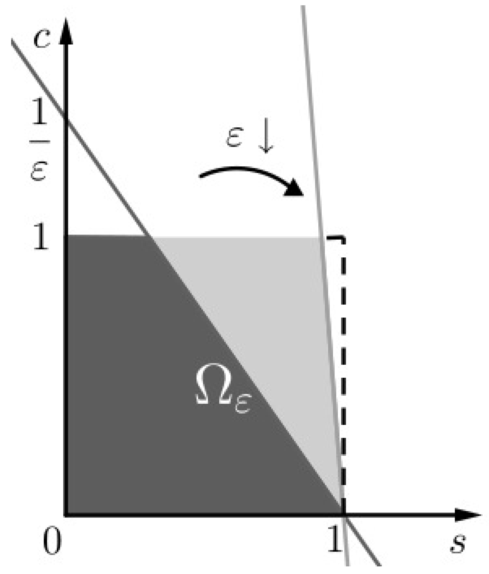
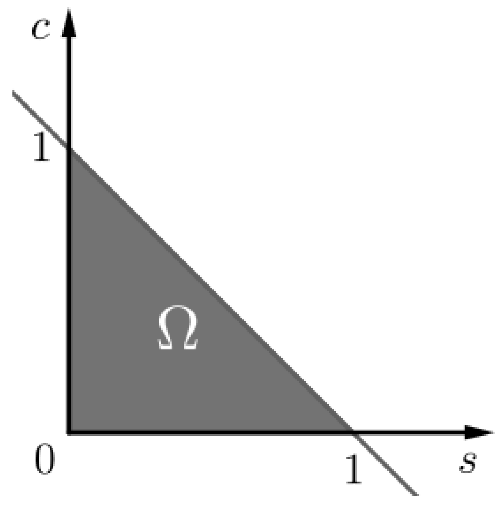
Figure 1. The invariant set ${\mathsf{\Omega }}_{\epsilon }$ of problem (SC_αs). We notice that ${\mathsf{\Omega }}_{\epsilon }\to {\left[0,1\right]}^2$ as $\epsilon \to 0^{+}$.

We study separately each of the two versions of (SC_αs) to find an inner and outer, respectively, approximation to the solution $\left(\left[S\right],\left[C\right]\right)$ of (SC), i.e., one approximation for times comparable to $t_1$ and another one for times comparable to $t_2$, respectively. In more detail:

• Looking at (SC) as a perturbed problem, with perturbation $\epsilon >0$ close to 0, we have the following information on (32a)

  $${\displaystyle \frac{\mathrm{d}{S}_{\alpha }}{\mathrm{d}{t}_{\alpha }}}=\underset{=O\left(\epsilon \right) \mathrm{uniformly} \mathrm{as} \epsilon \to 0^{+}}{\underbrace{\epsilon \left(\underset{\begin{array}{c}=O\left(1\right) \mathrm{uniformly} (\mathrm{with} \mathrm{respect} \mathrm{to} t_{\alpha }) \mathrm{as} \epsilon \to 0^{+},\\ \mathrm{since} \left(S_{\alpha },C_{\alpha },\right)=O\left(1\right) \mathrm{uniformly} \mathrm{as} \epsilon \to 0^{+},\\ \sin \mathrm{ce} \left(S_{\alpha },C_{\alpha }\right)\in {\mathsf{\Omega }}_{\epsilon } \forall \epsilon >0\end{array}}{\underbrace{-S_{\alpha }+\frac{\sigma }{1+\sigma }{S}_{\alpha }{C}_{\alpha }+\frac{\rho }{\left(1+\rho \right)\left(1+\sigma \right)}{C}_{\alpha }}}\right)}},$$

  as well as

  $$\underset{\begin{array}{c}=O\left(1\right) \mathrm{uniformly} \mathrm{as} \epsilon \to 0^{+},\\ \mathrm{when} t_{\alpha }=O\left(1\right) \mathrm{uniformly} \mathrm{as} \epsilon \to 0^{+},\\ \sin \mathrm{ce} S_{\alpha }=O\left(1\right) \mathrm{uniformly} \mathrm{as} \epsilon \to 0^{+}\\ \mathrm{combined} \mathrm{with} \mathrm{the} \mathrm{definition} \mathrm{of} \mathrm{the} \mathrm{derivative}\end{array}}{\underbrace{{\displaystyle \frac{\mathrm{d}{S}_{\alpha }}{\mathrm{d}{t}_{\alpha }}}}}=\underset{=O\left(\epsilon \right) \mathrm{uniformly} \mathrm{as} \epsilon \to 0^{+}}{\underbrace{\cdots }},$$

  thus

  $$\underset{\begin{array}{c}=O\left(\epsilon \right) \mathrm{uniformly} \mathrm{as} \epsilon \to 0^{+},\\ \mathrm{when} t_{\alpha }=O\left(1\right) \mathrm{uniformly} \mathrm{as} \epsilon \to 0^{+}\end{array}}{\underbrace{\frac{\mathrm{d}{S}_{\alpha }}{\mathrm{d}{t}_{\alpha }}}}.$$

  Thus, due to (28) it follows that:

  $$\frac{\mathrm{d}{S}_{\alpha }}{\mathrm{d}{t}_{\alpha }}\approx 0, \mathrm{when} \exists B>0 \mathrm{independent} \mathrm{of} \epsilon , \mathrm{such} \mathrm{that}: \left|t_{\alpha }\right|\le B,$$

  (34)

  and due to the initial condition of (SC_αs) we eventually have that:

  $$S_{\alpha }\approx \frac{{\left[S\right]}_0}{A_1}, \mathrm{when} \exists B>0: \left|t_{\alpha }\right|\le B.$$
  If we insert the above approximate equality in (32b), then the later becomes an approximate linear differential equation, the solution of which is:

  $$\begin{array}{cc}\hfill C_{\alpha }\approx \frac{\left(1+\sigma \right)S_{\alpha }}{1+\sigma S_{\alpha }}+\left({\displaystyle \frac{{\left[C\right]}_0}{\epsilon A_1}}-\frac{\left(1+\sigma \right)S_{\alpha }}{1+\sigma S_{\alpha }}\right)& exp\left\{-\frac{1+\sigma S_{\alpha }}{1+\sigma }{t}_{\alpha }\right\},\hfill \\ & \mathrm{when} \exists B>0: \left|t_{\alpha }\right|\le B,\hfill \end{array}$$

  given the initial condition of (SC_αs).
  Therefore, the inner approximation, $\left({\left[S\right]}_{\mathrm{in}},{\left[C\right]}_{\mathrm{in}}\right)$, of the solution $\left(\left[S\right],\left[C\right]\right)$ of (SC), i.e., the approximation for those t for which it holds that:

  $$\boxed{\exists B>0 \mathrm{independent} \mathrm{of} \epsilon , \mathrm{such} \mathrm{that}: \left|t\right|\le B{t}_1},$$

  is:

  $$\begin{array}{cc}\hfill {\left[S\right]}_{\mathrm{in}}& ={\left[S\right]}_0,\hfill \\ \hfill {\left[C\right]}_{\mathrm{in}}& =\frac{A_2{\left[S\right]}_0}{K_M+{\left[S\right]}_0}+\left({\left[C\right]}_0-\frac{A_2{\left[S\right]}_0}{K_M+{\left[S\right]}_0}\right)exp\left\{-k_1\left(K_M+{\left[S\right]}_0\right)t\right\}.\hfill \end{array}$$
• For (33b) we have that:

  $${\displaystyle \frac{\mathrm{d}{C}_{\alpha }}{\mathrm{d}{t}_{\alpha }}}=\underset{=O\left({\displaystyle \frac{1}{\epsilon }}\right) \mathrm{uniformly} \mathrm{as} \epsilon \to 0^{+}}{\underbrace{\frac{1}{\epsilon }\left(\underset{=O\left(1\right) \mathrm{uniformly} \mathrm{as} \epsilon \to 0^{+}}{\underbrace{S_{\alpha }-\frac{\sigma }{1+\sigma }{S}_{\alpha }{C}_{\alpha }-\frac{1}{1+\sigma }{C}_{\alpha }}}\right)}}$$

  as well as:

  $$\underset{\begin{array}{c}=O\left(1\right) \mathrm{uniformly} \mathrm{as} \epsilon \to 0^{+},\\ \mathrm{when} t_{\alpha }=O\left(1\right) \mathrm{uniformly} \mathrm{as} \epsilon \to 0^{+}\end{array}}{\underbrace{{\displaystyle \frac{\mathrm{d}{C}_{\alpha }}{\mathrm{d}{t}_{\alpha }}}}}=\underset{=O\left({\displaystyle \frac{1}{\epsilon }}\right) \mathrm{uniformly} \mathrm{as} \epsilon \to 0^{+}}{\underbrace{\cdots }},$$

  therefore, the stronger relation:

  $$\underset{\begin{array}{c}=O\left(\epsilon \right) \mathrm{uniformly} \mathrm{as} \epsilon \to 0^{+},\\ \mathrm{when} t_{\alpha }=O\left(1\right) \mathrm{uniformly} \mathrm{as} \epsilon \to 0^{+}\end{array}}{\underbrace{S_{\alpha }-\frac{\sigma }{1+\sigma }{S}_{\alpha }{C}_{\alpha }-\frac{1}{1+\sigma }{C}_{\alpha }}},$$

  holds. Thus, it follows that:

  $$\begin{array}{ccc}\hfill \epsilon \frac{\mathrm{d}{C}_{\alpha }}{\mathrm{d}{t}_{\alpha }}=S_{\alpha }-\frac{\sigma }{1+\sigma }& S_{\alpha }{C}_{\alpha }-\frac{1}{1+\sigma }{C}_{\alpha }\approx 0,\hfill & \\ & \mathrm{when} \exists B>0 \mathrm{independent} \mathrm{of} \epsilon , \mathrm{such} \mathrm{that}: \left|t_{\alpha }\right|\le B,\hfill \end{array}$$

  (35)

  i.e.:

  $$C_{\alpha }\approx \frac{\left(1+\sigma \right)S_{\alpha }}{1+\sigma S_{\alpha }}, \mathrm{when} \exists B>0 \mathrm{independent} \mathrm{of} \epsilon , \mathrm{such} \mathrm{that}: \left|t_{\alpha }\right|\le B.$$
  If we insert the above approximate equality in (33a), then the later becomes an approximate separable nonlinear differential equation, i.e.:

  $$\begin{array}{cc}\hfill \frac{\mathrm{d}{S}_{\alpha }}{\mathrm{d}{t}_{\alpha }}\approx -\frac{S_{\alpha }}{\left(1+\rho \right)\left(1+\sigma S_{\alpha }\right)},& \\ & \mathrm{when} \exists B>0 \mathrm{independent} \mathrm{of} \epsilon , \mathrm{such} \mathrm{that}: \left|t_{\alpha }\right|\le B,\hfill \end{array}$$

  (36)

  the solution of which is:

  $$S_{\alpha }\approx \frac{1}{\sigma }W\left(\sigma \ell exp\left\{\sigma \ell -\frac{1}{1+\rho }{t}_{\alpha }\right\}\right), \mathrm{when} \exists B>0: \left|t_{\alpha }\right|\le B,$$

  where W is the aforementioned Lambert function, and $\ell \ge 0$ is a constant that remains to be determined.
  Therefore, the outer approximation, $\left({\left[S\right]}_{\mathrm{out}},{\left[C\right]}_{\mathrm{out}}\right)$, of the solution $\left(\left[S\right],\left[C\right]\right)$ of (SC), i.e., the approximation for those t for which it holds that:

  $$\boxed{\exists B>0 \mathrm{independent} \mathrm{of} \epsilon , \mathrm{such} \mathrm{that}: \left|t\right|\le B{t}_2},$$

  is:

  $$\begin{array}{cc}\hfill {\left[S\right]}_{\mathrm{out}}& =K_{M}W\left(\frac{\ell A_1}{K_M}exp\left\{\frac{1}{K_M}\left(\ell A_1-k_2{A}_{2}t\right)\right\}\right),\hfill \\ \hfill {\left[C\right]}_{\mathrm{out}}& =\frac{A_{2}W\left(\frac{\ell A_1}{K_M}exp\left\{\frac{1}{K_M}\left(\ell A_1-k_2{A}_{2}t\right)\right\}\right)}{1+W\left(\frac{\ell A_1}{K_M}exp\left\{\frac{1}{K_M}\left(\ell A_1-k_2{A}_{2}t\right)\right\}\right)}.\hfill \end{array}$$

We can now utilize the matching technique in order to find a uniform approximation of the solution $\left(\left[S\right],\left[C\right]\right)$ of (SC) from the individual approximations $\left({\left[S\right]}_{\mathrm{in}},{\left[C\right]}_{\mathrm{in}}\right)$ and $\left({\left[S\right]}_{\mathrm{out}},{\left[C\right]}_{\mathrm{out}}\right)$. First, choosing a time scale between $t_1$ and $t_2$, e.g.:

$$\frac{t_1}{{\epsilon }^{\frac{1}{2}}}\in \left(t_1,t_2\right),$$

we find easily that the common limit resulting from the matching condition of the two individual solutions should be:

$$L:=\left({\left[S\right]}_0,\frac{A_2{\left[S\right]}_0}{K_M+{\left[S\right]}_0}\right).$$

Therefore:

$$\ell =\frac{{\left[S\right]}_0}{A_1}$$

and thus a uniform approximation $\left({\left[S\right]}_{\mathrm{un}},{\left[C\right]}_{\mathrm{un}}\right)$, of $\left(\left[S\right],\left[C\right]\right)$ is:

$$\left({\left[S\right]}_{\mathrm{un}},{\left[C\right]}_{\mathrm{un}}\right)=\left({\left[S\right]}_{\mathrm{in}},{\left[C\right]}_{\mathrm{in}}\right)+\left({\left[S\right]}_{\mathrm{out}},{\left[C\right]}_{\mathrm{out}}\right)-L,$$

i.e., in more detail:

$$\begin{array}{cc}\hfill {\left[S\right]}_{\mathrm{un}}& =K_{M}W\left(\frac{{\left[S\right]}_0}{K_M}exp\left\{\frac{1}{K_M}\left({\left[S\right]}_0-k_2{A}_{2}t\right)\right\}\right),\hfill \\ \hfill {\left[C\right]}_{\mathrm{un}}& =\frac{A_{2}W\left(\frac{{\left[S\right]}_0}{K_M}exp\left\{\frac{1}{K_M}\left({\left[S\right]}_0-k_2{A}_{2}t\right)\right\}\right)}{1+W\left(\frac{{\left[S\right]}_0}{K_M}exp\left\{\frac{1}{K_M}\left({\left[S\right]}_0-k_2{A}_{2}t\right)\right\}\right)}+\hfill \\ & +\left({\left[C\right]}_0-\frac{A_2{\left[S\right]}_0}{K_M+{\left[S\right]}_0}\right)exp\left\{-k_1\left(K_M+{\left[S\right]}_0\right)t\right\}.\hfill \end{array}$$

(37)

3.2. Total Substrate Approach

Since $\left(\left[S\right],\left[C\right]\right)\in {\mathsf{\Omega }}_1$, then $\left[T\right]\le A_1$, where $\left[T\right]$ is as in (15). Thus, we introduce, according to the third step, ${\mathfrak{A}}_3$, of algorithm ($\mathfrak{A}$), the dimensionless dependent variable

$$T_{\alpha }\left(t_{\alpha }\right):=\frac{1}{A_1}\left(\left[S\right]+\left[C\right]\right)\left(t_{\alpha }\right)=\left(S_{\alpha }+\epsilon C_{\alpha }\right)\left(t_{\alpha }\right).$$

The time scales $t_1$ and $t_2$ of the second step, ${\mathfrak{A}}_2$, of algorithm ($\mathfrak{A}$) have already been determined, thus (32) and (33) take the following forms:

• If $\boxed{t_{\alpha }={\displaystyle \frac{t}{t_1}}}$, then:

  $$\begin{array}{cc}\hfill {\displaystyle \frac{\mathrm{d}{T}_{\alpha }}{\mathrm{d}{t}_{\alpha }}}& =-\frac{\epsilon }{\left(1+\rho \right)\left(1+\sigma \right)}{C}_{\alpha },\hfill \end{array}$$

  (38a)

  $$\begin{array}{cc}\hfill {\displaystyle \frac{\mathrm{d}{C}_{\alpha }}{\mathrm{d}{t}_{\alpha }}}& =\frac{\epsilon \sigma }{1+\sigma }{C_{\alpha }}^2-\left(\frac{1}{1+\sigma }+\epsilon \right)C_{\alpha }-\frac{\sigma }{1+\sigma }{C}_{\alpha }{T}_{\alpha }+T_{\alpha }.\hfill \end{array}$$

  (38b)
• If $\boxed{t_{\alpha }={\displaystyle \frac{t}{t_2}}}$, then:

  $$\begin{array}{cc}\hfill {\displaystyle \frac{\mathrm{d}{T}_{\alpha }}{\mathrm{d}{t}_{\alpha }}}& =-\frac{1}{\left(1+\rho \right)\left(1+\sigma \right)}{C}_{\alpha },\hfill \end{array}$$

  (39a)

  $$\begin{array}{cc}\hfill {\displaystyle \frac{\mathrm{d}{C}_{\alpha }}{\mathrm{d}{t}_{\alpha }}}& =\frac{\sigma }{1+\sigma }{C_{\alpha }}^2-\left(\frac{1}{\epsilon \left(1+\sigma \right)}+1\right)C_{\alpha }-\frac{\sigma }{\epsilon \left(1+\sigma \right)}{C}_{\alpha }{T}_{\alpha }+\frac{1}{\epsilon }{T}_{\alpha }.\hfill \end{array}$$

  (39b)

So we have the following scaled problem:

$$\begin{array}{c}\mathit{Given} {\left[\mathit{S}\right]}_0,{\left[\mathit{C}\right]}_0,{\left[\mathit{P}\right]}_0\ge 0 \mathit{and} \epsilon >0, \mathit{we} \mathit{seek} \mathit{an} \mathit{interval} \mathcal{I}\subseteq \mathbb{R} \mathit{with} 0\in \mathcal{I}, \mathit{and}\\ \mathit{a} \mathit{function} \left({\mathit{T}}_{\alpha },{\mathit{C}}_{\alpha }\right):\mathcal{I}\to {\left[0,1\right]}^2, \mathit{such} \mathit{that} \left({\mathit{T}}_{\alpha },{\mathit{C}}_{\alpha }\right) \mathit{satisfies} \mathit{both}\left(38\right) \mathit{if}\\ {\mathit{t}}_{\alpha }={\displaystyle \frac{\mathit{t}}{{\mathit{t}}_1}}, \mathit{or}\left(39\right) \mathit{if} {\mathit{t}}_{\alpha }={\displaystyle \frac{\mathit{t}}{{\mathit{t}}_2}} \mathit{in} {\left(\mathcal{I}\setminus \left\{0\right\}\right)}^{\circ }, \mathit{and} \left({\mathit{T}}_{\alpha },{\mathit{C}}_{\alpha }\right)=\left({\displaystyle \frac{{\left[\mathit{S}\right]}_0}{{\mathit{A}}_1}}+{\displaystyle \frac{{\left[\mathit{C}\right]}_0}{\epsilon {\mathit{A}}_1}},{\displaystyle \frac{{\left[\mathit{C}\right]}_0}{\epsilon {\mathit{A}}_1}}\right),\\ \mathit{for} {\mathit{t}}_{\alpha }=0.\end{array}$$

(TC_αs)

Working as with problem (SC_αs), we conclude for problem (TC_αs) now, the following:

• (38a) gives that:

  $$\frac{\mathrm{d}{T}_{\alpha }}{\mathrm{d}{t}_{\alpha }}\approx 0, \mathrm{when} \exists B>0 \mathrm{independent} \mathrm{of} \epsilon , \mathrm{such} \mathrm{that}: \left|t_{\alpha }\right|\le B,$$

  and due to the initial condition of (TC_αs) we have that:

  $$T_{\alpha }\approx \frac{{\left[S\right]}_0}{A_1}+\frac{{\left[C\right]}_0}{\epsilon A_1}, \mathrm{when} \exists B>0: \left|t_{\alpha }\right|\le B.$$

  Inserting the above approximate equality into (38b), which in turn takes the following approximate form:

  $$\begin{array}{cc}\hfill \frac{\mathrm{d}{C}_{\alpha }}{\mathrm{d}{t}_{\alpha }}\approx -\left(\frac{\sigma }{1+\sigma }{T}_{\alpha }+\frac{1}{1+\sigma }\right)C_{\alpha }+T_{\alpha },& \\ & \mathrm{when} \exists B>0 \mathrm{independent} \mathrm{of} \epsilon , \mathrm{such} \mathrm{that}: \left|t_{\alpha }\right|\le B,\hfill \end{array}$$

  then the later becomes an approximate linear differential equation, the solution of which is:

  $$\begin{array}{cc}\hfill C_{\alpha }\approx \frac{\left(1+\sigma \right)T_{\alpha }}{1+\sigma T_{\alpha }}+\left({\displaystyle \frac{{\left[C\right]}_0}{\epsilon A_1}}-\frac{\left(1+\sigma \right)T_{\alpha }}{1+\sigma T_{\alpha }}\right)exp\left\{-\frac{1+\sigma T_{\alpha }}{1+\sigma }{t}_{\alpha }\right\},& \\ & \mathrm{when} \exists B>0: \left|t_{\alpha }\right|\le B,\hfill \end{array}$$

  given the initial condition of (TC_αs).
  Therefore, the inner approximation, $\left({\left[T\right]}_{\mathrm{in}},{\left[C\right]}_{\mathrm{in}}\right)$, of $\left(\left[T\right],\left[C\right]\right)$ is:

  $$\begin{array}{cc}\hfill {\left[T\right]}_{\mathrm{in}}& ={\left[T\right]}_0,\hfill \\ \hfill {\left[C\right]}_{\mathrm{in}}& =\frac{A_2{\left[T\right]}_0}{K_M+{\left[T\right]}_0}+\left({\left[C\right]}_0-\frac{A_2{\left[T\right]}_0}{K_M+{\left[T\right]}_0}\right)exp\left\{-k_1\left(K_M+{\left[T\right]}_0\right)t\right\},\hfill \end{array}$$

  where:

  $${\left[T\right]}_0:={\left[S\right]}_0+{\left[C\right]}_0.$$
• From (39b) we get that:

  $$\begin{array}{cc}\hfill \epsilon \left(\frac{\mathrm{d}{C}_{\alpha }}{\mathrm{d}{t}_{\alpha }}-\frac{\sigma }{1+\sigma }{C_{\alpha }}^2+C_{\alpha }\right)=-\frac{1}{1+\sigma }{C}_{\alpha }-\frac{\sigma }{1+\sigma }{C}_{\alpha }{T}_{\alpha }+T_{\alpha }\approx 0,& \\ & \mathrm{when} \exists B>0 \mathrm{independent} \mathrm{of} \epsilon , \mathrm{such} \mathrm{that}: \left|t_{\alpha }\right|\le B,\hfill \end{array}$$

  i.e.:

  $$C_{\alpha }\approx \frac{\left(1+\sigma \right)T_{\alpha }}{1+\sigma T_{\alpha }}, \mathrm{when} \exists B>0 \mathrm{independent} \mathrm{of} \epsilon , \mathrm{such} \mathrm{that}: \left|t_{\alpha }\right|\le B.$$

  If we insert the above approximate equality into (39a), then the later becomes an approximate separable nonlinear differential equation, namely:

  $$\begin{array}{cc}\hfill \frac{\mathrm{d}{T}_{\alpha }}{\mathrm{d}{t}_{\alpha }}\approx -\frac{T_{\alpha }}{\left(1+\rho \right)\left(1+\sigma T_{\alpha }\right)},& \\ & \mathrm{when} \exists B>0 \mathrm{independent} \mathrm{of} \epsilon , \mathrm{such} \mathrm{that}: \left|t_{\alpha }\right|\le B,\hfill \end{array}$$

  the solution of which is:

  $$T_{\alpha }\approx \frac{1}{\sigma }W\left(\sigma \ell exp\left\{\sigma \ell -\frac{1}{1+\rho }{t}_{\alpha }\right\}\right), \mathrm{when} \exists B>0: \left|t_{\alpha }\right|\le B,$$

  where $\ell \ge 0$ is a constant that remains to be determined. Therefore, the outer approximation $\left({\left[T\right]}_{\mathrm{out}},{\left[C\right]}_{\mathrm{out}}\right)$ of $\left(\left[T\right],\left[C\right]\right)$, is:

  $$\begin{array}{cc}\hfill {\left[T\right]}_{\mathrm{out}}& =K_{M}W\left(\frac{\ell A_1}{K_M}exp\left\{\frac{1}{K_M}\left(\ell A_1-k_2{A}_{2}t\right)\right\}\right),\hfill \\ \hfill {\left[C\right]}_{\mathrm{out}}& =\frac{A_{2}W\left(\frac{\ell A_1}{K_M}exp\left\{\frac{1}{K_M}\left(\ell A_1-k_2{A}_{2}t\right)\right\}\right)}{1+W\left(\frac{\ell A_1}{K_M}exp\left\{\frac{1}{K_M}\left(\ell A_1-k_2{A}_{2}t\right)\right\}\right)}.\hfill \end{array}$$

Finally, with a similar reasoning as for the uniform approximation of the solution of (SC), we have that:

$$\ell =\frac{{\left[T\right]}_0}{A_1}$$

and also that the uniform approximation, $\left({\left[T\right]}_{\mathrm{un}},{\left[C\right]}_{\mathrm{un}}\right)$, of $\left(\left[T\right],\left[C\right]\right)$ is:

$$\begin{array}{cc}\hfill {\left[T\right]}_{\mathrm{un}}& =K_{M}W\left(\frac{{\left[T\right]}_0}{K_M}exp\left\{\frac{1}{K_M}\left({\left[T\right]}_0-k_2{A}_{2}t\right)\right\}\right),\hfill \\ \hfill {\left[C\right]}_{\mathrm{un}}& =\frac{A_{2}W\left(\frac{{\left[T\right]}_0}{K_M}exp\left\{\frac{1}{K_M}\left({\left[T\right]}_0-k_2{A}_{2}t\right)\right\}\right)}{1+W\left(\frac{{\left[T\right]}_0}{K_M}exp\left\{\frac{1}{K_M}\left({\left[T\right]}_0-k_2{A}_{2}t\right)\right\}\right)}+\hfill \\ & +\left({\left[T\right]}_0-\frac{A_2{\left[T\right]}_0}{K_M+{\left[T\right]}_0}\right)exp\left\{-k_1\left(K_M+{\left[T\right]}_0\right)t\right\}.\hfill \end{array}$$

(40)

3.3. Conclusions

We showed that given (sQSSA) there is a $t_1>0$ such that:

$$\frac{\mathrm{d}\left[S\right]}{\mathrm{d}t}\approx 0, \mathrm{when} \exists B>0 \mathrm{independent} \mathrm{of} \epsilon , \mathrm{such} \mathrm{that}: \left|t\right|\le B{t}_1,$$

which arises directly from (34), as well as that there is a $t_2\gg t_1$ such that:

$$\frac{\mathrm{d}\left[C\right]}{\mathrm{d}t}\approx 0, \mathrm{when} \exists B>0 \mathrm{independent} \mathrm{of} \epsilon , \mathrm{such} \mathrm{that}: \left|t\right|\le B{t}_2,$$

which in turn results from (35).

In fact, due to (36) it holds that:

$$\frac{\mathrm{d}\left[S\right]}{\mathrm{d}t}\approx -\frac{k_2{A}_2\left[S\right]}{K_M+\left[S\right]}, \mathrm{when} \exists B>0: \left|t\right|\le B{t}_2.$$

Hence, we can conclude that:

$$\upsilon \approx \left\{\begin{array}{cc}0,\hfill & \mathrm{when} \exists B>0: \left|t\right|\le B{t}_1,\hfill \\ {\displaystyle \frac{k_2{A}_2\left[S\right]}{K_M+\left[S\right]}},\hfill & \mathrm{when} \exists B>0: \left|t\right|\le B{t}_2,\hfill \end{array}\right.$$

where $\upsilon$ is the rate of the chemical reaction with chemical Equation (1) (see Figure 2), i.e., nontrivial kinetics occur only in the outer layer (for t comparable to $t_2$). The above approximation for the outer layer is none other than the Michaelis–Menten approximation for the kinetics of the aforementioned chemical reaction, as already commented in (8).

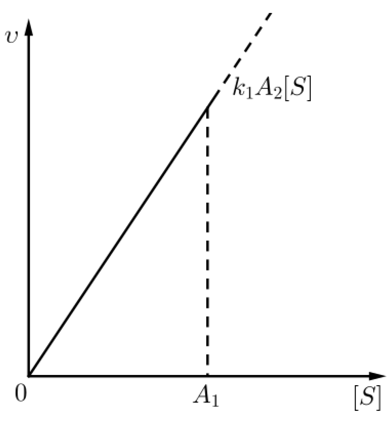
Figure 2. An approximation for the kinetics of the chemical reaction (1) given that (sQSSA) holds, for times in the outer layer.

Furthermore, comparing the approximate solution of the free substrate $\left({\left[S\right]}_{\mathrm{un}},{\left[C\right]}_{\mathrm{un}}\right)$ of (37) with the approximate solution of the total substrate $\left({\left[T\right]}_{\mathrm{un}},{\left[C\right]}_{\mathrm{un}}\right)$ of (40), these two should be in agreement. Indeed, it is sufficient to observe that:

$$\left[T\right]\approx \left[S\right],$$

as:

$$T_{\alpha }=S_{\alpha }+\epsilon C_{\alpha }\stackrel{\left(28\right)}{\approx }{S}_{\alpha }\Rightarrow T\approx S.$$

3.4. Numerical Verification

We numerically verify the above results, as shown in Figure 3, Figure 4 and Figure 5. For the numerical values of the constants and the initial conditions, we follow the work of Segel in 1988 [10]; these values are given in the following table .

Parameter	Value	Unit
$k_{-1}$	25	${\mathrm{s}}^{-1}$
$k_1$	$4\times {10}^6$	${\mathrm{M}}^{-1}{\mathrm{s}}^{-1}$
$k_2$	15	${\mathrm{s}}^{-1}$
${\left[S\right]}_0$	${10}^{-5}$	M
${\left[E\right]}_0$	${10}^{-8}$	M
${\left[C\right]}_0$	0	M
${\left[P\right]}_0$	0	M

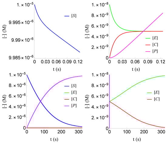
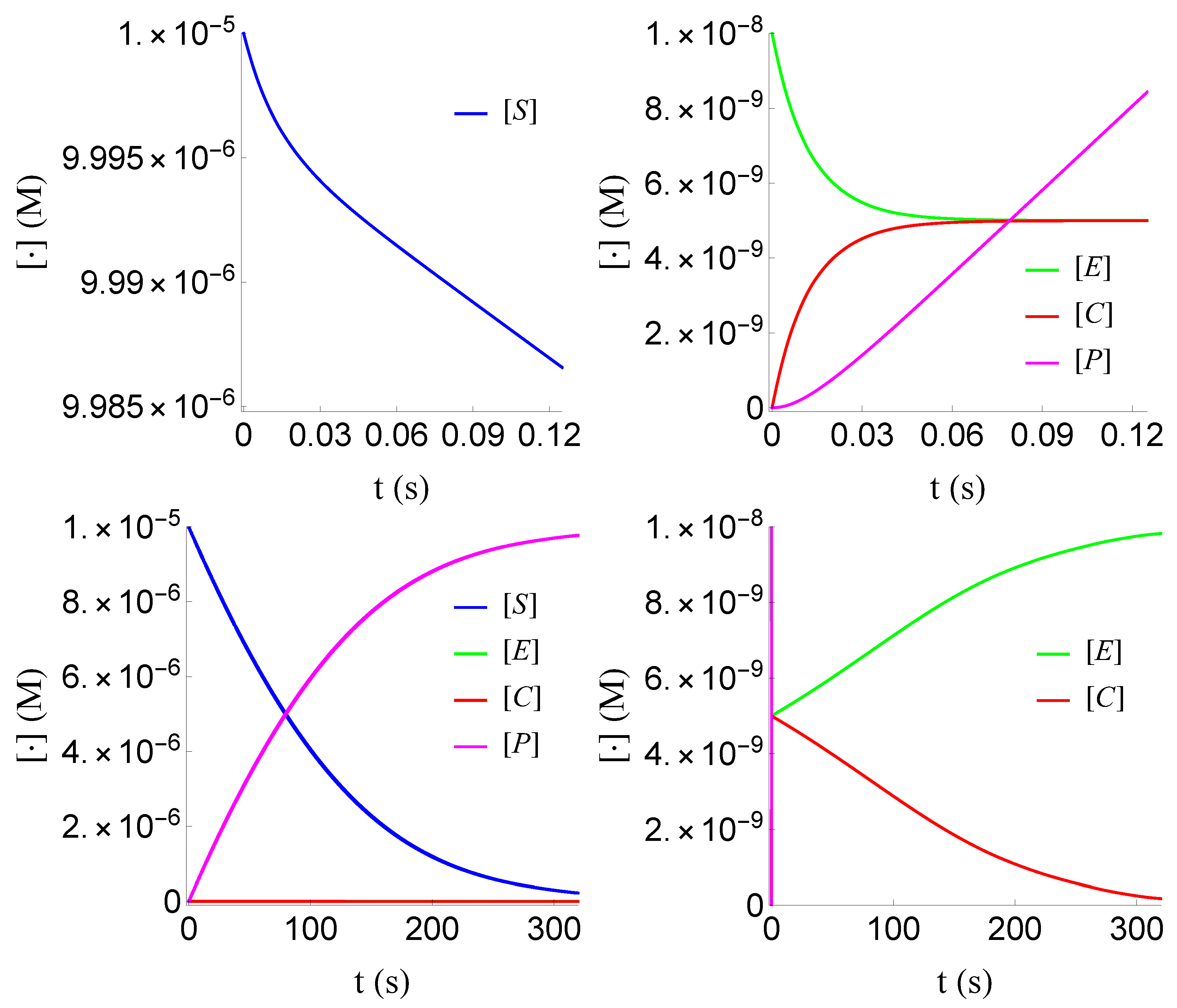
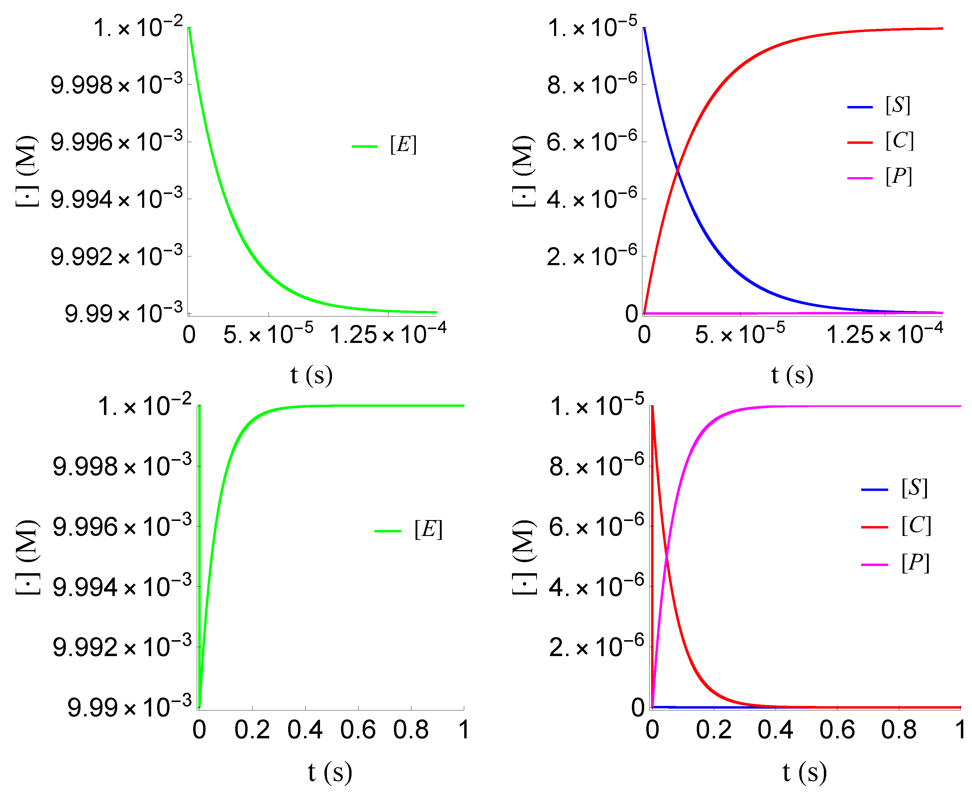
Figure 3. Plot of $\left[S\right]$, $\left[E\right]$, $\left[C\right]$ and $\left[P\right]$ of problem (SECP) for non-negative times, given that (sQSSA) holds. We see that $\left[S\right]$ and $\left[C\right]$ are of different order of magnitude, as well as that there are two distinct phases of the evolution of the phenomenon.

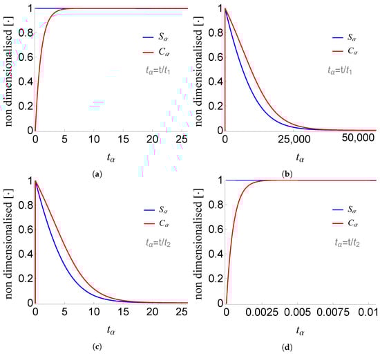
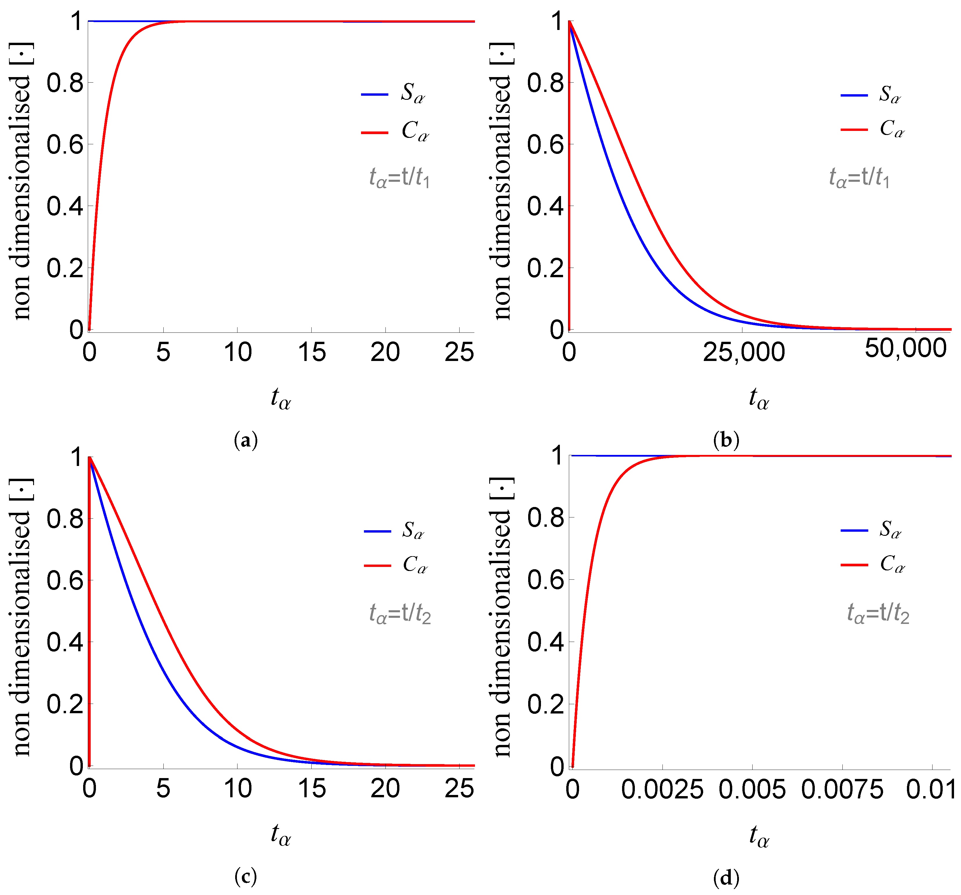
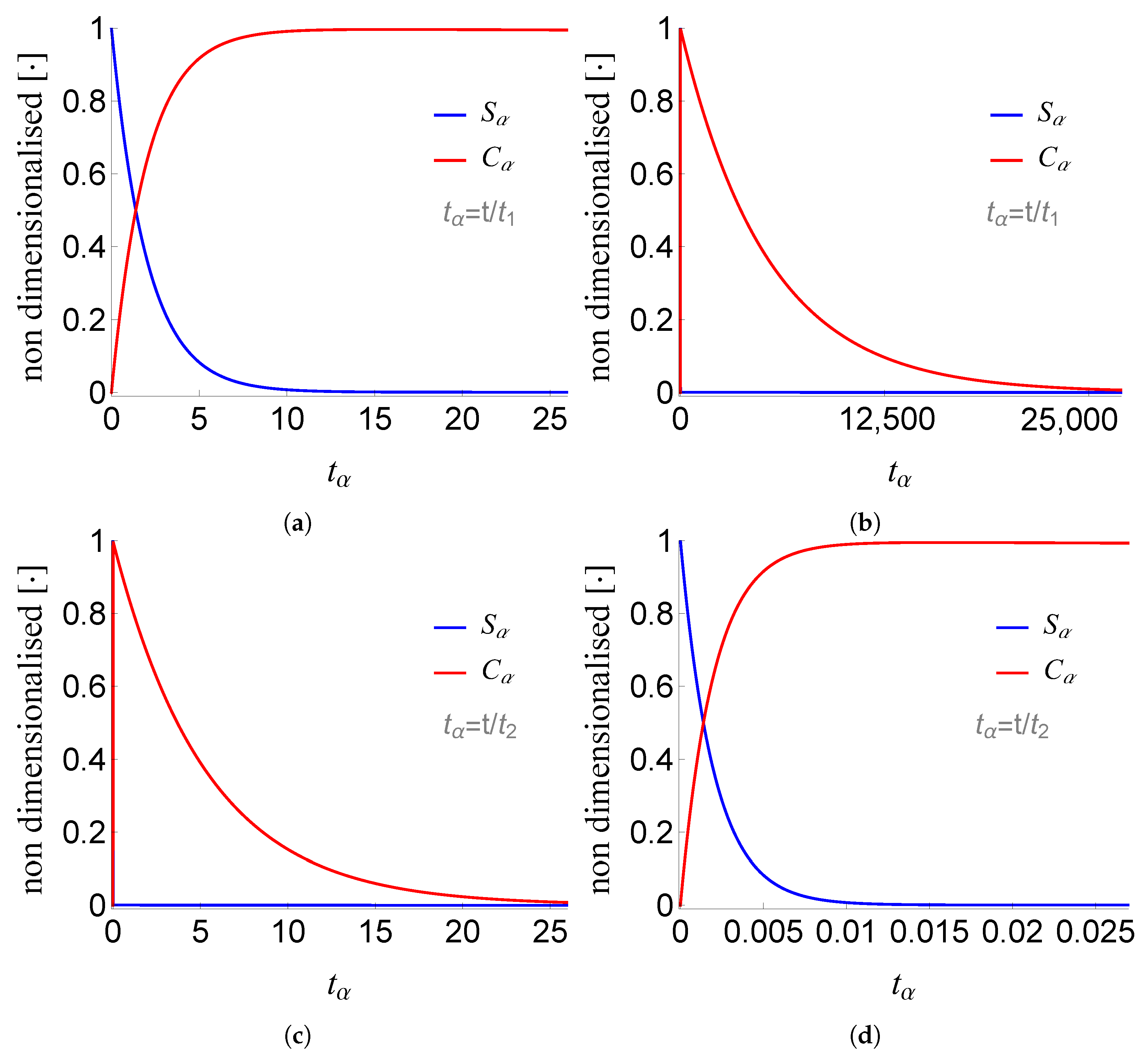
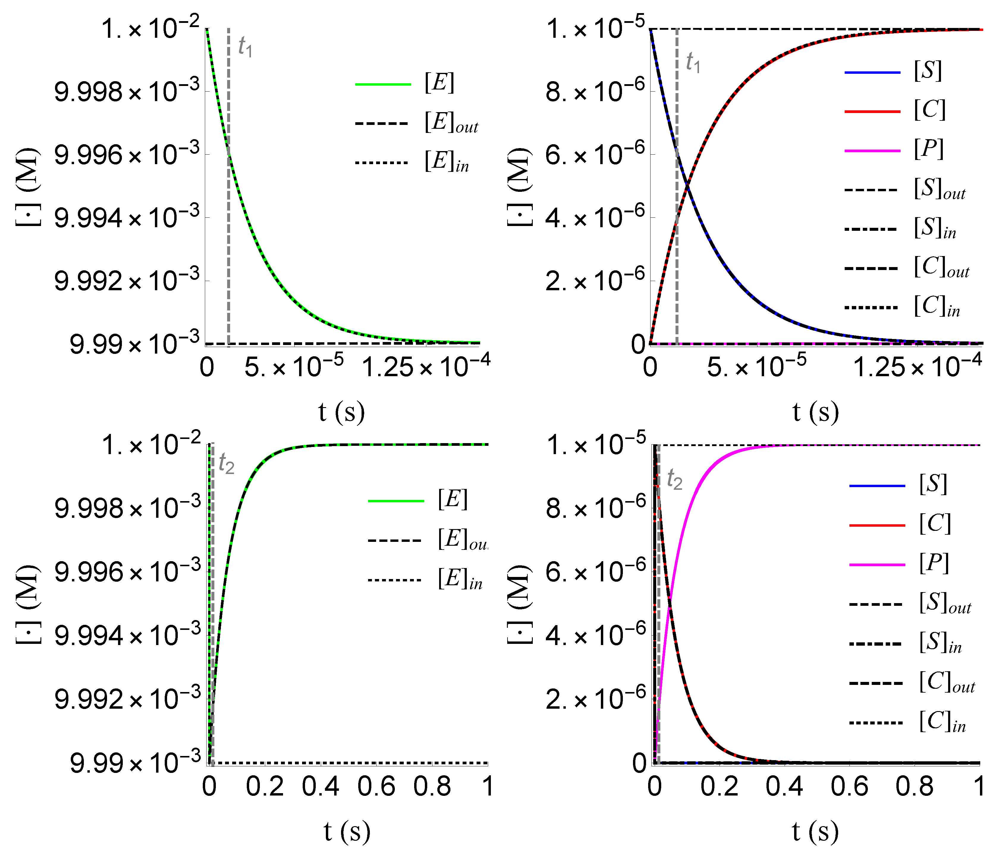
Figure 4. Plots of $S_{\alpha }$ and $C_{\alpha }$ of problem (SC_αs) for non-negative times, given that (sQSSA) holds. In (a) and (b) time is measured based on $t_1$, whereas in (c) and (d) based on $t_2$.

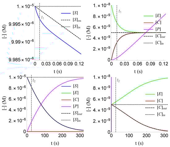
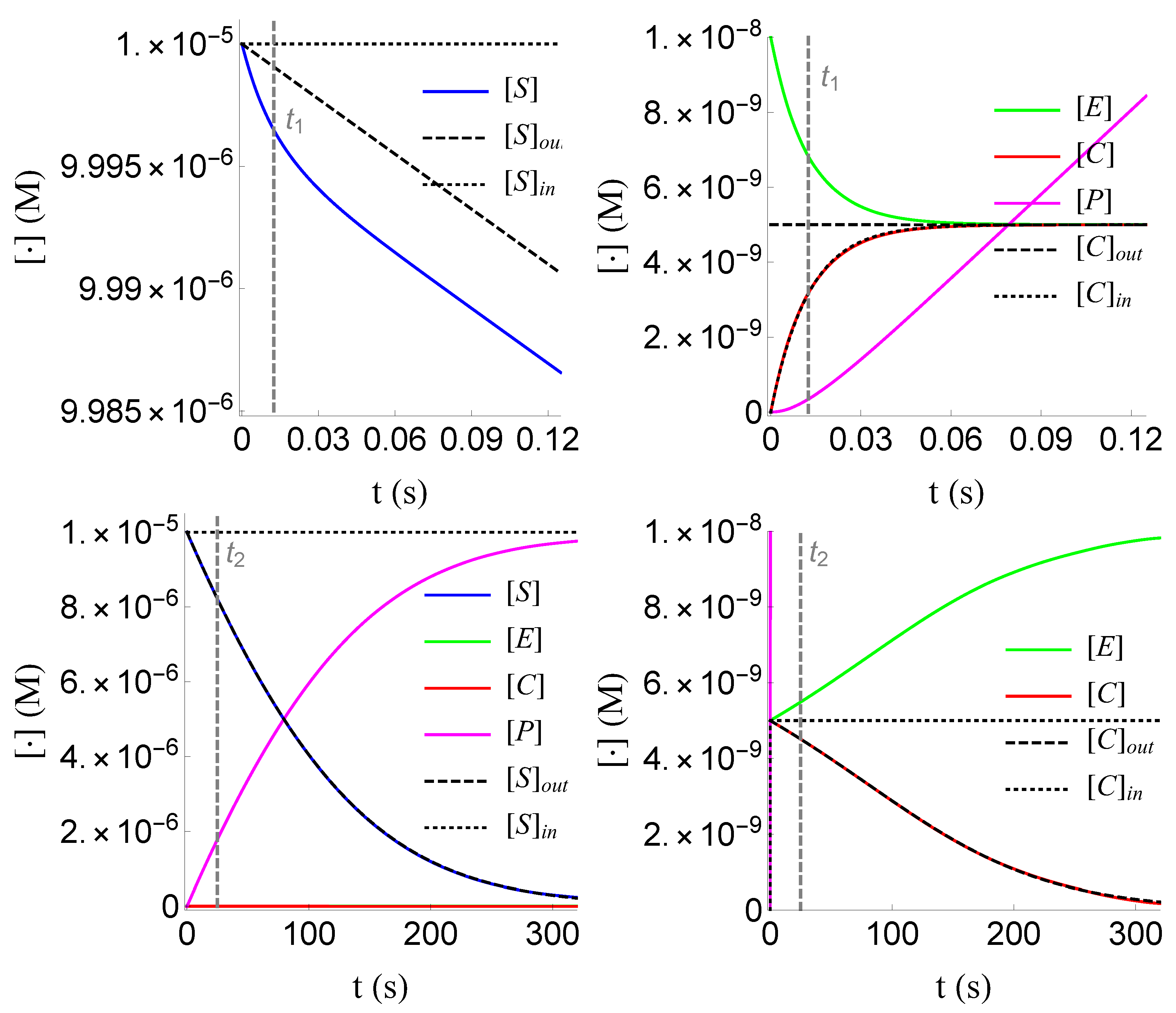
Figure 5. Plots of the inner and outer approximations of $\left[S\right]$ and $\left[C\right]$ of problem (SECP), for non-negative times, given that (sQSSA) holds.

In view of these:

$$K_M={\left[S\right]}_0=A_1 \mathrm{and} A_2={\left[E\right]}_0={10}^{-3}{\left[S\right]}_0={10}^{-3}{A}_1,$$

i.e.:

$$\epsilon =5\times {10}^{-4}$$

and:

$$t_1=1.25\times {10}^{-2} \mathrm{s} \mathrm{and} t_2=25 \mathrm{s}.$$

4. The Reverse Quasi-Steady-State Assumption

The reverse quasi-steady-state assumption is the following:

$$\boxed{A_1>0 \mathrm{and} A_2\gg K_M+A_1},$$

(rQSSA)

or, equivalently:

$$A_1>0, A_2\gg K_M \mathrm{and} A_2\gg A_1,$$

and given that this holds we study problem (SC).

We notice that the inequality $A_2\gg K_M+A_1$ of (rQSSA) is the reverse of the one corresponding to (sQSSA), hence the name of the first. As for the analysis of (sQSSA), here, as well, we consider two approaches for the study of case (rQSSA), the free substrate approach and the total substrate approach.

4.1. Free Substrate Approach

Using only (rQSSA) we will show that:

• Problem (SC), and therefore problem (SECP) as well, has inherently two time scales which we will determine. In particular, except for a short initial time interval where the enzymatic reaction with chemical Equation (1) is evolving with rate $\upsilon$, showing approximately linear behavior with respect to $\left[S\right]$, and $\upsilon \approx k_1{A}_2\left[S\right]$ as in (13), during the rest of the time the enzymatic reaction does not evolve, i.e., $\upsilon \approx 0$.
• There is a good uniform approximation in closed form to the solution of (SC), and therefore to (SECP) as well, which we will determine.

According to the second step, ${\mathfrak{A}}_2$, of algorithm ($\mathfrak{A}$), we use the dimensionless dependent variables:

$$S_{\alpha }\left(t_{\alpha }\right):=\frac{1}{A_1}\left[S\right]\left(\frac{t}{t_{*}}\right) \mathrm{and} C_{\alpha }\left(t_{\alpha }\right):=\frac{1}{A_4}\left[C\right]\left(\frac{t}{t_{*}}\right),$$

where we have chosen an arbitrary, for the time being, time scale $t_{*}>0$ for the scaling.

We notice, however, that given (rQSSA) it follows from (26) that:

$$\boxed{A_4=A_1}$$

and:

$$C_{\alpha }\left(t_{\alpha }\right)=\frac{1}{A_1}\left[C\right]\left(\frac{t}{t_{*}}\right).$$

A first conclusion is that the possible change of $\left[S\right]$ is comparable to the corresponding of $\left[C\right]$.

We set:

$$0\stackrel{\left(\mathit{rQSSA}\right)}{<}\eta :=\frac{A_1}{A_2}<\frac{K_M+A_1}{A_2}=\frac{1}{\epsilon }\stackrel{\left(\mathit{rQSSA}\right)}{\ll }1,$$

(41)

where $\epsilon$ is as in (27), i.e., equivalently:

$$0<\eta <\frac{1}{\epsilon }\approx 0,$$

(42)

and so (22) will take the following form:

$$\begin{array}{cc}\hfill {\displaystyle \frac{\mathrm{d}{S}_{\alpha }}{\mathrm{d}{t}_{\alpha }}}& =\frac{k_1\left(K_M+A_1\right)A_2}{A_1}{t}_{*}\left(-\frac{\sigma }{1+\sigma }{S}_{\alpha }+\frac{\eta \sigma }{1+\sigma }{S}_{\alpha }{C}_{\alpha }+\frac{\eta \rho }{\left(1+\rho \right)\left(1+\sigma \right)}{C}_{\alpha }\right),\hfill \end{array}$$

(43a)

$$\begin{array}{cc}\hfill {\displaystyle \frac{\mathrm{d}{C}_{\alpha }}{\mathrm{d}{t}_{\alpha }}}& =\frac{k_1\left(K_M+A_1\right)A_2}{A_1}{t}_{*}\left(\frac{\sigma }{1+\sigma }{S}_{\alpha }-\frac{\eta \sigma }{1+\sigma }{S}_{\alpha }{C}_{\alpha }-\frac{\eta }{1+\sigma }{C}_{\alpha }\right),\hfill \end{array}$$

(43b)

where $\sigma$ and $\rho$ are as in (30).

According to the third step, ${\mathfrak{A}}_3$, of algorithm ($\mathfrak{A}$), in view of (43) we define:

$$\frac{A_1}{k_1\left(K_M+A_1\right)A_2}=:t_1\stackrel{\left(41\right)}{\ll }\frac{t_1}{\eta }=\frac{1}{k_1\left(K_M+A_1\right)}=:t_2,$$

(44)

to conclude that:

$$t_{*}=t_1\Rightarrow \frac{k_1\left(K_M+A_1\right)A_2}{A_1}{t}_{*}=1 \mathrm{and} t_{*}=t_2\Rightarrow \frac{k_1\left(K_M+A_1\right)A_2}{A_1}{t}_{*}=\frac{1}{\eta },$$

so as (43) gets the following forms:

• If $\boxed{t_{\alpha }={\displaystyle \frac{t}{t_1}}}$, then:

  $$\begin{array}{cc}\hfill {\displaystyle \frac{\mathrm{d}{S}_{\alpha }}{\mathrm{d}{t}_{\alpha }}}& =-\frac{\sigma }{1+\sigma }{S}_{\alpha }+\frac{\eta \sigma }{1+\sigma }{S}_{\alpha }{C}_{\alpha }+\frac{\eta \rho }{\left(1+\rho \right)\left(1+\sigma \right)}{C}_{\alpha },\hfill \end{array}$$

  (45a)

  $$\begin{array}{cc}\hfill {\displaystyle \frac{\mathrm{d}{C}_{\alpha }}{\mathrm{d}{t}_{\alpha }}}& =\frac{\sigma }{1+\sigma }{S}_{\alpha }-\frac{\eta \sigma }{1+\sigma }{S}_{\alpha }{C}_{\alpha }-\frac{\eta }{1+\sigma }{C}_{\alpha }.\hfill \end{array}$$

  (45b)
• If $\boxed{t_{\alpha }={\displaystyle \frac{t}{t_2}}}$, then:

  $$\begin{array}{cc}\hfill {\displaystyle \frac{\mathrm{d}{S}_{\alpha }}{\mathrm{d}{t}_{\alpha }}}& =-\frac{\sigma }{\eta \left(1+\sigma \right)}{S}_{\alpha }+\frac{\sigma }{1+\sigma }{S}_{\alpha }{C}_{\alpha }+\frac{\rho }{\left(1+\rho \right)\left(1+\sigma \right)}{C}_{\alpha },\hfill \end{array}$$

  (46a)

  $$\begin{array}{cc}\hfill {\displaystyle \frac{\mathrm{d}{C}_{\alpha }}{\mathrm{d}{t}_{\alpha }}}& =\frac{\sigma }{\eta \left(1+\sigma \right)}{S}_{\alpha }-\frac{\sigma }{1+\sigma }{S}_{\alpha }{C}_{\alpha }-\frac{1}{1+\sigma }{C}_{\alpha }.\hfill \end{array}$$

  (46b)

Setting (see Figure 6):

$$\mathsf{\Omega }:=\left\{\left(s,c\right)\in {\left[0,1\right]}^2|s+c\le 1\right\},$$

the scaled version of (SC) will be as follows:

$$\begin{array}{c}\mathit{Given} {\left[\mathit{S}\right]}_0,{\left[\mathit{C}\right]}_0,{\left[\mathit{P}\right]}_0\ge 0 \mathit{and} \eta >0, \mathit{we} \mathit{seek} \mathit{an} \mathit{interval} \mathcal{I}\subseteq \mathbb{R} \mathit{with} 0\in \mathcal{I}, \mathit{and}\\ \mathit{a} \mathit{function} \left({\mathit{S}}_{\alpha },{\mathit{C}}_{\alpha }\right):\mathcal{I}\to \mathsf{\Omega }, \mathit{such} \mathit{that} \left({\mathit{S}}_{\alpha },{\mathit{C}}_{\alpha }\right) \mathit{satisfies} \mathit{both} \left(45\right) \mathit{if} {\mathit{t}}_{\alpha }={\displaystyle \frac{\mathit{t}}{{\mathit{t}}_1}}, \mathit{or}\\ \left(46\right) \mathit{if} {\mathit{t}}_{\alpha }={\displaystyle \frac{\mathit{t}}{{\mathit{t}}_2}} \mathit{in} {\left(\mathcal{I}\setminus \left\{0\right\}\right)}^{\circ }, \mathit{and} \left({\mathit{S}}_{\alpha },{\mathit{C}}_{\alpha }\right)=\left({\displaystyle \frac{{\left[\mathit{S}\right]}_0}{{\mathit{A}}_1}},{\displaystyle \frac{{\left[\mathit{C}\right]}_0}{{\mathit{A}}_1}}\right), \mathit{for} {\mathit{t}}_{\alpha }=0.\end{array}$$

(SC_αr)

Figure 6. The invariant set $\mathsf{\Omega }$ of problem (SC_αr).

We study each of two versions of (SC_αr) separately:

• From (45a), which due to (42) takes the approximate linear form:

  $$\frac{\mathrm{d}{S}_{\alpha }}{\mathrm{d}{t}_{\alpha }}\approx -\frac{\sigma }{1+\sigma }{S}_{\alpha }, \mathrm{when} \exists B>0 \mathrm{independent} \mathrm{of} \eta , \mathrm{such} \mathrm{that}: \left|t_{\alpha }\right|\le B,$$

  (47)

  we get, due to the initial condition of (SC_αr), that:

  $$S_{\alpha }\approx \frac{{\left[S\right]}_0}{A_1}exp\left\{-\frac{\sigma }{1+\sigma }{t}_{\alpha }\right\}, \mathrm{when} \exists B>0: \left|t_{\alpha }\right|\le B.$$

  If we insert the above approximate equality in (45b), which will now have the approximate form:

  $${\displaystyle \frac{\mathrm{d}{C}_{\alpha }}{\mathrm{d}{t}_{\alpha }}}\approx \frac{\sigma }{1+\sigma }{S}_{\alpha }, \mathrm{when} \exists B>0: \left|t_{\alpha }\right|\le B,$$

  then we get that:

  $$C_{\alpha }\approx \frac{{\left[C\right]}_0}{A_1}+\frac{{\left[S\right]}_0}{A_1}\left(1-exp\left\{-\frac{\sigma }{1+\sigma }{t}_{\alpha }\right\}\right), \mathrm{when} \exists B>0: \left|t_{\alpha }\right|\le B,$$

  given the initial condition of (SC_αr). Therefore, the inner approximation, $\left({\left[S\right]}_{\mathrm{in}},{\left[C\right]}_{\mathrm{in}}\right)$, of $\left(\left[S\right],\left[C\right]\right)$ is:

  $$\left({\left[S\right]}_{\mathrm{in}},{\left[C\right]}_{\mathrm{in}}\right)=\left({\left[S\right]}_{0}exp\left\{-k_1{A}_{2}t\right\},{\left[C\right]}_0+{\left[S\right]}_0\left(1-exp\left\{-k_1{A}_{2}t\right\}\right)\right).$$
• From (46a) we have that:

  $$\begin{array}{cc}\hfill \eta \left(\frac{\mathrm{d}{S}_{\alpha }}{\mathrm{d}{t}_{\alpha }}-\frac{\sigma }{1+\sigma }{S}_{\alpha }{C}_{\alpha }-\frac{\rho }{\left(1+\rho \right)\left(1+\sigma \right)}{C}_{\alpha }\right)=-\frac{\sigma }{1+\sigma }{S}_{\alpha }\approx 0,& \\ & \mathrm{when} \exists B>0 \mathrm{independent} \mathrm{of} \eta , \mathrm{such} \mathrm{that}: \left|t_{\alpha }\right|\le B,\hfill \end{array}$$

  (48)

  i.e.:

  $$S_{\alpha }\approx 0, \mathrm{when} \exists B>0: \left|t_{\alpha }\right|\le B,$$

  thus:

  $$\frac{\mathrm{d}{S}_{\alpha }}{\mathrm{d}{t}_{\alpha }}\approx 0, \mathrm{when} \exists B>0: \left|t_{\alpha }\right|\le B.$$

  If we insert the above approximate equality in the sum of (46a) and (46b), then the following approximate linear differential equation arises:

  $$\begin{array}{cc}\hfill \frac{\mathrm{d}{C}_{\alpha }}{\mathrm{d}{t}_{\alpha }}\approx -\frac{1}{\left(1+\rho \right)\left(1+\sigma \right)}{C}_{\alpha },& \\ & \mathrm{when} \exists B>0 \mathrm{independent} \mathrm{of} \eta , \mathrm{such} \mathrm{that}: \left|t_{\alpha }\right|\le B,\hfill \end{array}$$

  the solution of which is:

  $$C_{\alpha }\approx \ell exp\left\{-\frac{1}{(1+\rho )(1+\sigma )}{t}_{\alpha }\right\}, \mathrm{when} \exists B>0: \left|t_{\alpha }\right|\le B,$$

  where $\ell \ge 0$ a constant that remains to be determined. Therefore, the external approximation, $\left({\left[S\right]}_{\mathrm{out}},{\left[C\right]}_{\mathrm{out}}\right)$, of $\left(\left[S\right],\left[C\right]\right)$ is:

  $$\left({\left[S\right]}_{\mathrm{out}},{\left[C\right]}_{\mathrm{out}}\right)=\left(0,\ell A_{1}exp\left\{-k_{2}t\right\}\right).$$

Finally, as usual, we find that:

$$\ell =\frac{{\left[S\right]}_0}{A_1}+\frac{{\left[C\right]}_0}{A_1},$$

as well as that the uniform approximation, $\left({\left[S\right]}_{\mathrm{un}},{\left[C\right]}_{\mathrm{un}}\right)$, of $\left(\left[S\right],\left[C\right]\right)$ is:

$$\begin{array}{cc}\hfill {\left[S\right]}_{\mathrm{un}}& ={\left[S\right]}_{0}exp\left\{-k_1{A}_{2}t\right\},\hfill \\ \hfill {\left[C\right]}_{\mathrm{un}}& ={\left[C\right]}_{0}exp\left\{-k_{2}t\right\}+{\left[S\right]}_0\left(exp\left\{-k_{2}t\right\}-exp\left\{-k_1{A}_{2}t\right\}\right).\hfill \end{array}$$

(49)

4.2. Total Substrate Approach

Since $\left(\left[S\right],\left[C\right]\right)\in {\mathsf{\Omega }}_1$, we have that $\left[T\right]\le A_1$. Thus, we introduce, according to the second step, ${\mathfrak{A}}_2$, of algorithm ($\mathfrak{A}$), the dimensionless dependent variable:

$$T_{\alpha }\left(t_{\alpha }\right):=\frac{1}{A_1}\left(\left[S\right]+\left[C\right]\right)\left(t_{\alpha }\right)=\left(S_{\alpha }+C_{\alpha }\right)\left(t_{\alpha }\right).$$

The time scales $t_1$ and $t_2$ of the third step, ${\mathfrak{A}}_3$, of algorithm ($\mathfrak{A}$) have already been determined, thus (45) and (46) get the following forms:

• If $\boxed{t_{\alpha }={\displaystyle \frac{t}{t_1}}}$, then:

  $$\begin{array}{cc}\hfill {\displaystyle \frac{\mathrm{d}{T}_{\alpha }}{\mathrm{d}{t}_{\alpha }}}& =-\frac{\eta }{\left(1+\rho \right)\left(1+\sigma \right)}{C}_{\alpha },\hfill \end{array}$$

  (50a)

  $$\begin{array}{cc}\hfill {\displaystyle \frac{\mathrm{d}{C}_{\alpha }}{\mathrm{d}{t}_{\alpha }}}& =\frac{\eta \sigma }{1+\sigma }{C_{\alpha }}^2-\frac{\eta +\sigma }{1+\sigma }{C}_{\alpha }-\frac{\eta \sigma }{1+\sigma }{C}_{\alpha }{T}_{\alpha }+\frac{\sigma }{1+\sigma }{T}_{\alpha }.\hfill \end{array}$$

  (50b)
• If $\boxed{t_{\alpha }={\displaystyle \frac{t}{t_2}}}$, then:

  $$\begin{array}{cc}\hfill {\displaystyle \frac{\mathrm{d}{T}_{\alpha }}{\mathrm{d}{t}_{\alpha }}}& =-\frac{1}{\left(1+\rho \right)\left(1+\sigma \right)}{C}_{\alpha },\hfill \end{array}$$

  (51a)

  $$\begin{array}{cc}\hfill {\displaystyle \frac{\mathrm{d}{C}_{\alpha }}{\mathrm{d}{t}_{\alpha }}}& =\frac{\sigma }{1+\sigma }{C_{\alpha }}^2-\frac{\eta +\sigma }{\eta \left(1+\sigma \right)}{C}_{\alpha }-\frac{\sigma }{1+\sigma }{C}_{\alpha }{T}_{\alpha }+\frac{\sigma }{\eta \left(1+\sigma \right)}{T}_{\alpha }.\hfill \end{array}$$

  (51b)

So we have the following scaled problem:

$$\begin{array}{c}\mathit{Given} {\left[\mathit{S}\right]}_0,{\left[\mathit{C}\right]}_0,{\left[\mathit{P}\right]}_0\ge 0 \mathit{and} \eta >0, \mathit{we} \mathit{seek} \mathit{an} \mathit{interval} \mathcal{I}\subseteq \mathbb{R} \mathit{with} 0\in \mathcal{I}, \mathit{and}\\ \mathit{a} \mathit{function} \left({\mathit{T}}_{\alpha },{\mathit{C}}_{\alpha }\right):\mathcal{I}\to {\left[0,1\right]}^2, \mathit{such} \mathit{that} \left({\mathit{T}}_{\alpha },{\mathit{C}}_{\alpha }\right) \mathit{satisfies} \mathit{both} \left(50\right) \mathit{if}\\ {\mathit{t}}_{\alpha }={\displaystyle \frac{\mathit{t}}{{\mathit{t}}_1}}, \mathit{or} \left(51\right) \mathit{if} {\mathit{t}}_{\alpha }={\displaystyle \frac{\mathit{t}}{{\mathit{t}}_2}} \mathit{in} {\left(\mathcal{I}\setminus \left\{0\right\}\right)}^{\circ }, \mathit{and} \left({\mathit{T}}_{\alpha },{\mathit{C}}_{\alpha }\right)=\left({\displaystyle \frac{{\left[\mathit{T}\right]}_0}{{\mathit{A}}_1}},{\displaystyle \frac{{\left[\mathit{C}\right]}_0}{{\mathit{A}}_1}}\right), \mathit{for}\\ {\mathit{t}}_{\alpha }=0.\end{array}$$

(TC_αr)

Working as with problem (SC_αr), we conclude, now for problem (TC_αr), the following:

• (50a) gives that:

  $$\frac{\mathrm{d}{T}_{\alpha }}{\mathrm{d}{t}_{\alpha }}\approx 0, \mathrm{when} \exists B>0 \mathrm{independent} \mathrm{of} \eta , \mathrm{such} \mathrm{that}: \left|t_{\alpha }\right|\le B,$$

  and due to the initial condition of (TC_αr) we have that:

  $$T_{\alpha }\approx \frac{{\left[T\right]}_0}{A_1}, \mathrm{when} \exists B>0: \left|t_{\alpha }\right|\le B.$$

  If we insert the above approximate equality into (50b), which will now have the approximate linear form:

  $$\begin{array}{cc}\hfill {\displaystyle \frac{\mathrm{d}{C}_{\alpha }}{\mathrm{d}{t}_{\alpha }}}\approx -\frac{\sigma }{1+\sigma }{C}_{\alpha }+\frac{\sigma }{1+\sigma }{T}_{\alpha },& \\ & \mathrm{when} \exists B>0 \mathrm{independent} \mathrm{of} \eta , \mathrm{such} \mathrm{that}: \left|t_{\alpha }\right|\le B,\hfill \end{array}$$

  then we will get:

  $$C_{\alpha }\approx T_{\alpha }+\left(\frac{{\left[C\right]}_0}{A_1}-T_{\alpha }\right)exp\left\{-\frac{\sigma }{1+\sigma }{t}_{\alpha }\right\}, \mathrm{when} \exists B>0: \left|t_{\alpha }\right|\le B,$$

  given the initial condition (TC_αr).
  Therefore, the initial condition, $\left({\left[T\right]}_{\mathrm{in}},{\left[C\right]}_{\mathrm{in}}\right)$, of $\left(\left[T\right],\left[C\right]\right)$ is:

  $$\left({\left[T\right]}_{\mathrm{in}},{\left[C\right]}_{\mathrm{in}}\right)=\left({\left[T\right]}_0,{\left[T\right]}_0+\left({\left[C\right]}_0-{\left[T\right]}_0\right)exp\left\{-k_1{A}_{2}t\right\}\right).$$
• From (51b) we obtain that:;

  $$\begin{array}{cc}\hfill \eta \left(\frac{\mathrm{d}{C}_{\alpha }}{\mathrm{d}{t}_{\alpha }}-\frac{\sigma }{1+\sigma }{C_{\alpha }}^2+\frac{1}{1+\sigma }{C}_{\alpha }-\frac{\sigma }{1+\sigma }{C}_{\alpha }{T}_{\alpha }\right)=\frac{\sigma }{1+\sigma }\left(-C_{\alpha }+T_{\alpha }\right)\approx 0,& \\ & \mathrm{when} \exists B>0 \mathrm{independent} \mathrm{of} \eta , \mathrm{such} \mathrm{that}: \left|t_{\alpha }\right|\le B,\hfill \end{array}$$

  i.e.,

  $$T_{\alpha }\approx C_{\alpha }, \mathrm{when} \exists B>0 \mathrm{independent} \mathrm{of} \eta , \mathrm{such} \mathrm{that}: \left|t_{\alpha }\right|\le B.$$

  If we insert the above approximate equality in (51a), then the later becomes an approximate linear differential equation, which is none other than:

  $$\begin{array}{cc}\hfill \frac{\mathrm{d}{T}_{\alpha }}{\mathrm{d}{t}_{\alpha }}\approx -\frac{1}{\left(1+\rho \right)\left(1+\sigma \right)}{T}_{\alpha },& \\ & \mathrm{when} \exists B>0 \mathrm{independent} \mathrm{of} \eta , \mathrm{such} \mathrm{that}: \left|t_{\alpha }\right|\le B,\hfill \end{array}$$

  the solution of which is

  $$T_{\alpha }\approx \ell exp\left\{-\frac{1}{(1+\rho )(1+\sigma )}{t}_{\alpha }\right\}, \mathrm{when} \exists B>0: \left|t_{\alpha }\right|\le B,$$

  where $\ell \ge 0$ a constant that remains to be determined. Therefore, the outer approximation, $\left({\left[T\right]}_{\mathrm{out}},{\left[C\right]}_{\mathrm{out}}\right)$, of $\left(\left[T\right],\left[C\right]\right)$ is

  $$\begin{array}{c}\hfill \left({\left[T\right]}_{\mathrm{out}},{\left[C\right]}_{\mathrm{out}}\right)=\left(\ell A_{1}exp\left\{-k_{2}t\right\},\ell A_{1}exp\left\{-k_{2}t\right\}\right).\end{array}$$

Finally, as usually, we find that

$$\ell =\frac{{\left[T\right]}_0}{A_1},$$

as well as that the uniform approximation, $\left({\left[T\right]}_{\mathrm{un}},{\left[C\right]}_{\mathrm{un}}\right)$, of $\left(\left[T\right],\left[C\right]\right)$ is

$$\begin{array}{cc}\hfill {\left[T\right]}_{\mathrm{un}}& ={\left[T\right]}_{0}exp\left\{-k_{2}t\right\},\hfill \\ \hfill {\left[C\right]}_{\mathrm{un}}& ={\left[T\right]}_{0}exp\left\{-k_{2}t\right\}+\left({\left[C\right]}_0-{\left[T\right]}_0\right)exp\left\{-k_1{A}_{2}t\right\}.\hfill \end{array}$$

(52)

4.3. Conclusions

Although for the previous analysis it was used that $0<\eta \approx 0,$ i.e.,

$$A_1\ll A_2,$$

nevertheless we emphasize that also the relation:

$$K_M\ll A_2,$$

(53)

even though it does not directly appear in the appropriately scaled Equations (45) and (46) (as well as in (50) and (51)), it plays an essential role in distinguishing (rQSSA) from (sQSSA). Indeed, let:

$$K_{M}N=(1,1)A_2,$$

i.e.:

$$K_M\gg A_2, \mathrm{or} K_M\approx A_2.$$

Then, given that we have $A_1\ll A_2$, we conclude that:

$$\left\{\begin{array}{cc}{A}_2\ll K_M+A_1,\hfill & \mathrm{if} K_M\gg A_2\gg A_1, \mathrm{or}\hfill \\ A_2\approx K_M+A_1,\hfill & \mathrm{if} K_M\approx A_2\gg A_1.\hfill \end{array}\right.$$

The first case falls into (sQSSA), while the second represents neither (rQSSA) nor (sQSSA). We note that the above—easily explained—role of (53) in distinguishing the aforementioned assumptions, has been recently studied in a—rather complex—context of geometric singular perturbation theory (see, e.g., [24,25] and the references therein).

In addition, we showed that given (rQSSA) there is $t_1>0$ such that:

$$\frac{\mathrm{d}\left[S\right]}{\mathrm{d}t}\approx -k_1{A}_2\left[S\right], \mathrm{when} \exists B>0 \mathrm{independent} \mathrm{of} \eta , \mathrm{such} \mathrm{that}: \left|t\right|\le B{t}_1,$$

which arises directly from (47), as well as that there is $t_2\gg t_1$ such that;

$$\frac{\mathrm{d}\left[S\right]}{\mathrm{d}t}\approx \left[S\right]\approx 0, \mathrm{when} \exists B>0 \mathrm{independent} \mathrm{of} \eta , \mathrm{such} \mathrm{that}: \left|t\right|\le B{t}_2,$$

which in turn results from (48). i.e., we can conclude that:

$$\upsilon \approx \left\{\begin{array}{cc}{k}_1{A}_2\left[S\right],\hfill & \mathrm{when} \exists B>0: \left|t\right|\le B{t}_1,\hfill \\ 0,\hfill & \mathrm{when} \exists B>0: \left|t\right|\le B{t}_2,\hfill \end{array}\right.$$

where $\upsilon$ stands for the rate of the chemical reaction with chemical Equation (1), as we have already mentioned (see Figure 7), i.e., non trivial kinetics occur only in the inner layer (for t comparable to $t_1$).

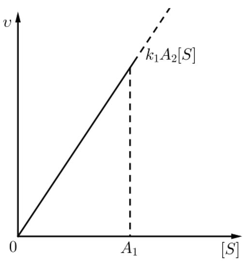
Figure 7. An approximation for the kinetics of the chemical reaction (1) given that (rQSSA) holds, for times in the inner layer.

Finally, comparing the approximate solution of the free substrate $\left({\left[S\right]}_{\mathrm{un}},{\left[C\right]}_{\mathrm{un}}\right)$ of (49) with the approximate solution of the total substrate $\left({\left[T\right]}_{\mathrm{un}},{\left[C\right]}_{\mathrm{un}}\right)$ of (52), we easily observe by definition in (15) that they are in agreement.

4.4. Numerical Verification

We numerically verify the above results, as shown in Figure 8, Figure 9 and Figure 10. For the numerical values of the constants and the initial conditions we follow the work of Segel in 1988 [10]; these values are given in the following table .

Parameter	Value	Unit
$k_{-1}$	25	s${}^{-1}$
$k_1$	$4\times {10}^6$	M${}^{-1}$s${}^{-1}$
$k_2$	15	s${}^{-1}$
${\left[S\right]}_0$	${10}^{-5}$	M
${\left[E\right]}_0$	${10}^{-2}$	M
${\left[C\right]}_0$	0	M
${\left[P\right]}_0$	0	M

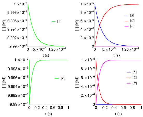
Figure 8. Plots of $\left[S\right]$, $\left[E\right]$, $\left[C\right]$ and $\left[P\right]$ of problem (SECP) for times, given that (rQSSA) holds. We see that $\left[S\right]$ and $\left[C\right]$ are of the same order of magnitude, as well as that there are two distinct phases of the evolution of the phenomenon.

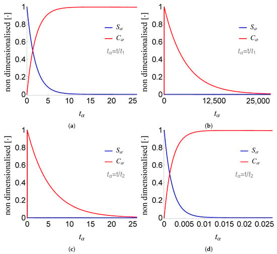
Figure 9. Plots of $S_{\alpha }$ and $C_{\alpha }$ of problem (SC_αr) for non-negative times, given that (rQSSA) holds. In (a) and (b) time is measured based on $t_1$, whereas (c) and (d) based on $t_2$.

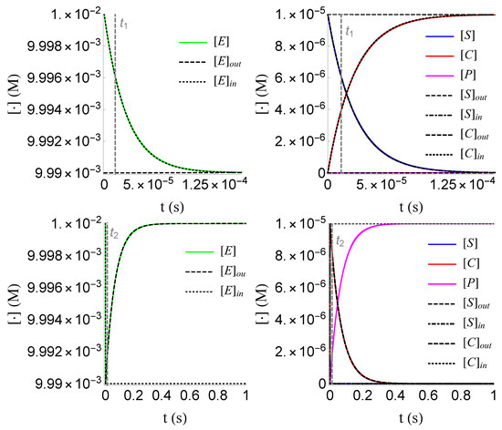
Figure 10. Plots of the inner and outer approximations of $\left[S\right]$, $\left[E\right]$ and $\left[C\right]$ of problem (SECP), for non-negative times, given that (sQSSA) holds. The inner and outer approximation of $\left[E\right]$ are given by the relations ${\left[E\right]}_{\mathrm{in}}=A_2-{\left[C\right]}_{\mathrm{in}}$ and ${\left[E\right]}_{\mathrm{out}}=A_2-{\left[C\right]}_{\mathrm{out}}$, respectively, due to (18).

In view of these,

$$K_M={\left[S\right]}_0=A_1 \mathrm{and} A_2={\left[E\right]}_0={10}^3{\left[S\right]}_0={10}^3{A}_1,$$

i.e.,

$$\epsilon =500, \frac{1}{\epsilon }=2\times {10}^{-3} \mathrm{and} \eta ={10}^{-3}$$

and

$$t_1=1.25\times {10}^{-5} \mathrm{s} \mathrm{and} t_2=1.25\times {10}^{-2} \mathrm{s}.$$

5. Discussion

• We repeatedly (i.e., Section 2.2, Section 3.1, Section 3.2, Section 4.1 and Section 4.2) employed the scaling algorithm ($\mathfrak{A}$) for the rigorous treatment of the quasi-steady-state assumption. We note that such an algorithm can be utilised in all problems having non-negative solutions in a bounded domain. Another typical such example is the simple classical $SIR$ problem of Epidemiology

  $$\begin{array}{cc}\hfill {\displaystyle \frac{\mathrm{d}S}{\mathrm{d}t}}& =-\beta SI,\hfill \\ \hfill {\displaystyle \frac{\mathrm{d}I}{\mathrm{d}t}}& =-\gamma I+\beta SI,\hfill \\ \hfill {\displaystyle \frac{\mathrm{d}R}{\mathrm{d}t}}& =\gamma I,\hfill \end{array}$$

  for $\beta ,\gamma >0$, where the feasible region is the set

  $$\left\{\left(s,i,r\right)\in {\left[0,N_0\right]}^3|s+i+r=N_0\right\},$$

  (first step, ${\mathfrak{A}}_1$, of algorithm ($\mathfrak{A}$)), hence every dependent variable, S, I and R, is scaled by $N_0$ (second step, ${\mathfrak{A}}_2$, of algorithm ($\mathfrak{A}$)), and the above system then becomes

  $$\begin{array}{cc}\hfill \frac{1}{\gamma }{\displaystyle \frac{\mathrm{d}{S}_{\alpha }}{\mathrm{d}t}}& =-{\displaystyle \frac{\beta N_0}{\gamma }}{S}_{\alpha }{I}_{\alpha },\hfill \\ \hfill \frac{1}{\gamma }{\displaystyle \frac{\mathrm{d}{I}_{\alpha }}{\mathrm{d}t}}& =-I_{\alpha }+{\displaystyle \frac{\beta N_0}{\gamma }}{S}_{\alpha }{I}_{\alpha },\hfill \\ \hfill \frac{1}{\gamma }{\displaystyle \frac{\mathrm{d}{R}_{\alpha }}{\mathrm{d}t}}& =I_{\alpha }.\hfill \end{array}$$

  By such an approach we naturally obtain the time scale to be ${\displaystyle \frac{1}{\gamma }}$ (third step, ${\mathfrak{A}}_3$, of algorithm ($\mathfrak{A}$)) and, using the well known non dimensionalized quantity

  $${\mathcal{R}}_0={\displaystyle \frac{\beta N_0}{\gamma }},$$

  the fully scaled equations finally get the form

  $$\begin{array}{cc}\hfill {\displaystyle \frac{\mathrm{d}{S}_{\alpha }}{\mathrm{d}{t}_{\alpha }}}& =-{\mathcal{R}}_0{S}_{\alpha }{I}_{\alpha },\hfill \\ \hfill {\displaystyle \frac{\mathrm{d}{I}_{\alpha }}{\mathrm{d}{t}_{\alpha }}}& =-I_{\alpha }+{\mathcal{R}}_0{S}_{\alpha }{I}_{\alpha },\hfill \\ \hfill {\displaystyle \frac{\mathrm{d}{R}_{\alpha }}{\mathrm{d}{t}_{\alpha }}}& =I_{\alpha }.\hfill \end{array}$$
• From the basic mathematical analysis of (SECP), we were able to generate in an elegant way the quantity $\epsilon$ that characterises both (sQSSA) and (rQSSA). Moreover, we determined, in a natural way, two pairs of distinctive time scales, each pair of which is characteristic for each one of the aforementioned two assumptions.
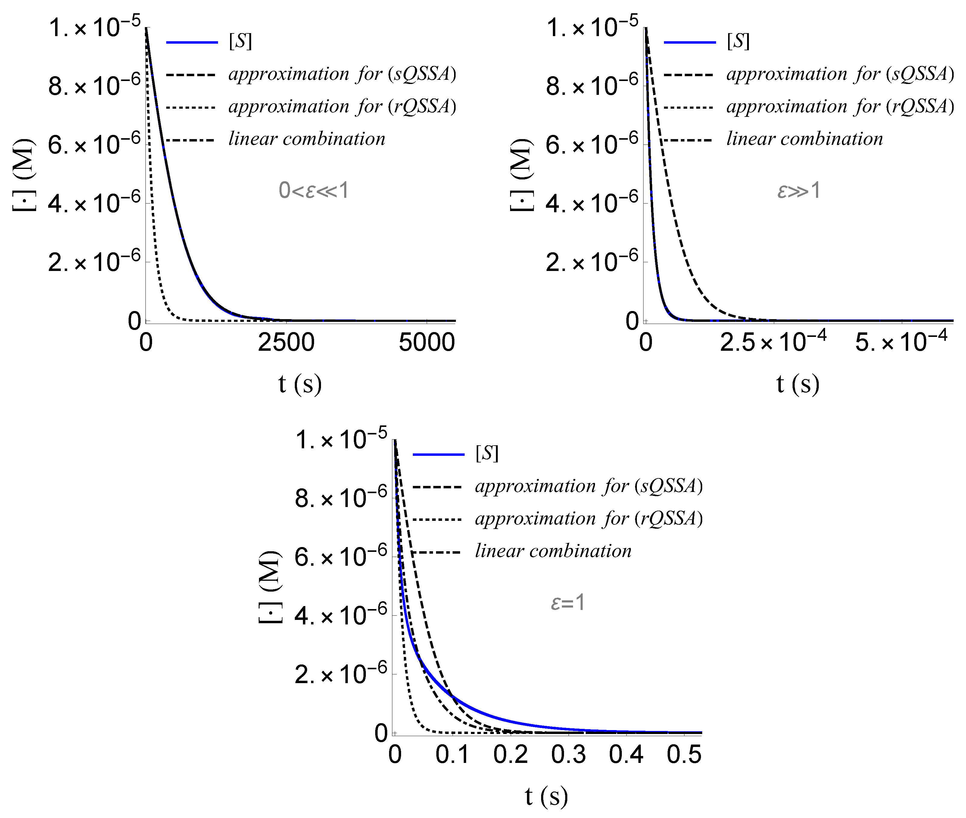
• We obtained a good approximation of the solution in closed form, for both the cases where $\epsilon \to 0^{+}$ and $\epsilon \to \infty$, which we can communally write as

  $$\frac{\epsilon }{1+\epsilon }\times \left(\mathrm{approximation} \mathrm{for} \epsilon \to \infty \right)+\left(1-\frac{\epsilon }{1+\epsilon }\right)\times \left(\mathrm{approximation} \mathrm{for} \epsilon \to 0^{+}\right).$$
  We emphasize that the above linear combination is far from being a good approximation of the solution for the case where $\epsilon \sim 1$, as it is illustrated in Figure 11. Such an approximation requires a much more sophisticated extrapolation technique, the study of which lies beyond the scope of the present work.
  

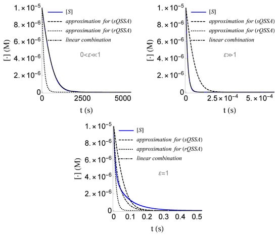  Figure 11. For a good approximation of the solution of (SECP) for the case where $\epsilon \sim 1$, a sophisticated extrapolation technique is required, than just a linear combination of the approximations of the solution for (sQSSA) and (rQSSA).

References

- Fischer, E. Einfluss der Configuration auf die Wirkung der Enzyme. Berichte Dtsch. Der Chem. Ges. 1894, 27, 2985–2993. [Google Scholar] [CrossRef] [Green Version]
- Brown, A.J. Enzyme action. J. Chem. Soc. 1902, 81, 373–388. [Google Scholar] [CrossRef] [Green Version]
- Henri, V. Über das gesetz der wirkung des invertins. Z. für Phys. Chem. 1902, 39, 194–216. [Google Scholar] [CrossRef]
- Henri, V. Lois Générales de l’Action des Diastases; Librairie Scientifique A. Hermann: Paris, France, 1903. [Google Scholar]
- Michaelis, L.; Menten, M.L. Die kinetik der invertinwirkung. Biochem. Z. 1913, 49, 333–369. [Google Scholar]
- Johnson, K.A.; Goody, R.S. The Original Michaelis Constant: Translation of the 1913 Michaelis-Menten Paper. Biochemistry 2011, 50, 8264–8269. [Google Scholar] [CrossRef] [PubMed] [Green Version]
- Van Slyke, D.D.; Cullen, G.E. The mode of Action of urease and of enzymes in general. J. Biol. Chem. 1914, 19, 141–180. [Google Scholar] [CrossRef]
- Briggs, G.E.; Haldane, J.B.S. A note on the kinetics of enzyme action. Biochem. J. 1925, 19, 338–339. [Google Scholar] [CrossRef] [PubMed] [Green Version]
- Lineweaver, H.; Burk, D. The determination of enzyme dissociation constants. J. Am. Chem. Soc. 1934, 56, 658–666. [Google Scholar] [CrossRef]
- Segel, L.A. On the validity of the steady state assumption of enzyme kinetics. Bull. Math. Biol. 1988, 50, 579–593. [Google Scholar] [CrossRef]
- Segel, L.A.; Slemrod, M. The quasi-steady-state assumption: A case study in perturbation. SIAM Rev. 1989, 31, 446–477. [Google Scholar] [CrossRef]
- Schnell, S.; Mendoza, C. Closed form solution for time-dependent enzyme kinetics. J. Theor. Biol. 1997, 187, 207–212. [Google Scholar] [CrossRef]
- Schnell, S.; Maini, P.K. Enzyme kinetics at high enzyme concentration. Bull. Math. Biol. 2000, 62, 483–499. [Google Scholar] [CrossRef] [PubMed] [Green Version]
- Borghans, J.A.M.; De Boer, R.J.; Segel, L.A. Extending the quasi-steady state approximation by changing variables. Bull. Math. Biol. 1996, 58, 43–63. [Google Scholar] [CrossRef] [PubMed]
- Logan, D.J. Applied Mathematics, 4th ed.; John Wiley & Sons: Hoboken, NJ, USA, 2013. [Google Scholar]
- Lin, C.C.; Segel, L.A. Mathematics Applied to Deterministic Problems in the Natural Sciences; SIAM: Philadelphia, PA, USA, 1988. [Google Scholar]
- Hale, J.K. Ordinary Differential Equations, 2nd ed.; Krieger Publishing Company: Malabar, FL, USA, 1980. [Google Scholar]
- Meiss, J.D. Differential Dynamical Systems, revised ed.; SIAM: Philadelphia, PA, USA, 2017. [Google Scholar]
- Pontryagin, L.S. Ordinary Differential Equations; Addison Wesley: Boston, MA, USA, 1962. [Google Scholar]
- Strogatz, S.H. Nonlinear Dynamics and Chaos: With Applications to Physics, Biology, Chemistry, and Engineering, 2nd ed.; CRC Press: Boca Raton, FL, USA, 2018. [Google Scholar]
- Bender, C.M.; Orszag, S.A. Advanced Mathematical Methods for Scientists and Engineers I: Asymptotic Methods and Perturbation Theory; Springer Science & Business Media: Berlin/Heidelberg, Germany, 2013. [Google Scholar]
- Holmes, M.H. Introduction to Perturbation Methods; Springer Science & Business Media: Berlin/Heidelberg, Germany, 2012. [Google Scholar]
- Voit, E.O.; Martens, H.A.; Omholt, S.W. 150 years of the mass action law. PLoS Comput. Biol. 2015, 11, e1004012. [Google Scholar] [CrossRef] [PubMed] [Green Version]
- Eilertsen, J.; Schnell, S.; Walcher, S. On the anti-quasi-steady-state conditions of enzyme kinetics. arXiv 2021, arXiv:2112.04098. [Google Scholar]
- Eilertsen, J.; Schnell, S. The quasi-steady-state approximations revisited: Timescales, small parameters, singularities, and normal forms in enzyme kinetics. Math. Biosci. 2020, 325, 108339. [Google Scholar] [CrossRef] [PubMed] [Green Version]
Publisher’s Note: MDPI stays neutral with regard to jurisdictional claims in published maps and institutional affiliations. |
© 2022 by the authors. Licensee MDPI, Basel, Switzerland. This article is an open access article distributed under the terms and conditions of the Creative Commons Attribution (CC BY) license (https://creativecommons.org/licenses/by/4.0/).