Abstract
In today’s world, the countries that have easy access to energy resources are economically strong, and thus, maintaining a better geopolitical position is important. Petroleum products such as gas and oil are currently the leading energy resources. Due to their excessive worth, the petroleum industries face many risks and security threats. Observing the nature of such problems, it is asserted that the complex bipolar fuzzy information is a better choice for modeling them. Keeping the said problem in mind, this article introduces the novel structure of complex bipolar fuzzy relation (CBFR), which is basically used to find out the relationships between complex bipolar fuzzy sets (CBFSs). Similarly, the types of CBFRs are also defined, which is helpful during the process of analyzing and interpreting the problem. Moreover, some useful results and interesting properties of the proposed structures are deliberated. Further, a new modeling technique based on the proposed structures is initiated, which is used to investigate the security risks to petroleum industries. Furthermore, a detailed comparative analysis proves the advantages and supremacy of CBFRs over other structures. Therefore, the results achieved by the proposed methods are substantially reliable, practical and complete.
Keywords:
fuzzy sets; bipolar fuzzy sets; complex bipolar fuzzy sets; complex bipolar fuzzy relation; oil and gas sectors; security of petroleum industries; terrorist attacks MSC:
03E99; 90B50
1. Introduction
In mathematics, modeling is the process of representing practical problems and events in a mathematical format or language. There are plenty of techniques for carrying out mathematical modeling. When it comes to modeling uncertainty, indistinctness and inaccuracy, fuzzy set theory and fuzzy logic are the right choices because they have the right tools for the said purpose. This theory was introduced by Zadeh [1] in 1965. A fuzzy set is a collection of objects that are assigned fuzzy value (real numbers between and , inclusively) mappings. This numerical value defies the partial membership of the elements to the fuzzy set. Afterward, this theory caught the attention of researchers worldwide. Today, the fuzzy set theory is mainly used for decision-making processes. Kandel and Byatt [2] wrote a research article on fuzzy sets (FSs), fuzzy statistics and fuzzy algebra. Robinson [3] described the fundamentals of FSs and their usages in geographic information systems. Yang et al. [4] showed the use of FSs in database acquisition. Kabir and Papadopoulos [5] reviewed the applications of FSs for safe and reliable engineering. Mardani et al. [6] applied FSs-based decision making (DM) to assess medical problems and healthcare. Mishra et al. [7] comprehended the fuzzy DM framework for choosing drugs to treat COVID-19 with mild symptoms, and Khalil et al. [8] proposed fuzzy logical algebra with its application to the effectiveness of medications for COVID-19.
Ramot et al. [9] reformed the structure of FSs by altering its membership mapping values from real numbers to complex numbers. The extended structure is called the complex FS (CFS). Hence, a CFS is a collection of objects that is assigned a complex valued mapping with a modulus less than or equal to . The complex numbers are more often written in exponential form. The coefficient of exponential function is called the amplitude term, whose value is a fuzzy number, and the exponent is called the phase term, which also takes on values from a unit interval . Due to its complex structure, a CFS can model multivariable problems. The phase term usually refers to phase-altering variables such as time phase or periodicity. A CFS is a generalization of FS, as the CFS with phase term value becomes an FS. Ma et al. [10] proposed a method that uses CFSs for prediction problems, i.e., multiple periodic factor prediction. Tamura et al. [11] first used FRs for pattern classification, and Yang and Shih [12] further extended it in cluster analysis. In 2003, Ramot et al. [13] formulated a complex FR (CFR) between two CFSs. Yazdanbakhsh and Dick [14] analyzed an organized review of CFSs and logic. Ali et al. [15] applied CFSs in the TOPSIS method. Nasir et al. [16] defined interval-valued CFRs and applied their method for studying the medical diagnoses and life expectancies of patients. Jan et al. [17,18,19] analyzed cybersecurity and cyber-threats using the extensions of CFRs.
Zhang [20] further generalized FSs and defined the concept of bipolar FSs (BFSs). A BFS is composed of objects carrying a pair of numbers; the positive membership mapping that takes on values form a unit interval and the negative membership mapping, which takes on the values from , thus allowing the modeling of objects that possess dual properties. Each of the membership mapping represents two different and opposing properties of an object. Zhang [21] also proposed the YinYang BFSs. Abdullah et al. [22] introduced the BF soft sets (BFSSs) and applied them in DM problems. Sarwar and Akram [23] offered the concept of bipolar fuzzy circuits and discussed their applications. Akram and Arshad [24] showed the bipolar fuzzy ELECTRE-I and TOPSIS methods for diagnosis. Lee and Hur [25] considered bipolar FRs (BFRs). Ali et al. [26] presented the attribute reductions of BFR decision systems. Alkouri et al. [27] extended BFSs to complex BFSs (CBFSs) with their applications. The advancement in the structure of CBFSs is the inclusion of complex valued positive and negative membership mappings. This improvement permitted the CBFS to model multidimensional uncertainty problems of periodic nature. Akram et al. [28] considered the solution of a CBF linear system. Gulistan et al. [29] applied CBFSs to a transport company, and Mahmood and Rehman [30] showed the applications of CBFSs in generalized similarity measures. Aliannezhadi et al. [31] showed an algorithm for the solution of linear programming-related problems of BFRs. Dutta and Doley [32] proposed a medical diagnosis under BFSs.
This article initiates complex bipolar fuzzy relations (CBFRs) as a generalization of CBFRs, CFRs and FRs. These concepts have similar structures as CBFSs—a pair of objects taking two complex values as their positive and negative membership mappings. This concept will help to find out the relation between CBFSs. Substituting phase terms equal to in CBFR makes it a BFR. When the negative membership mapping’s value is zero in a CBFR, then it becomes a CFR. For zero phase term and zero negative membership value, CBFR converts to a FR. Thus, a CBFR is a supreme tool that can handle all sorts of information. In addition, the Cartesian product between two CBFSs is also formulated. Furthermore, the types of CBFRs such as complex bipolar fuzzy reflexive relation, complex bipolar fuzzy irreflexive relation, complex bipolar fuzzy symmetric relation complex bipolar fuzzy antisymmetric relation, complex bipolar fuzzy transitive relation, complex bipolar fuzzy equivalence relation, complex bipolar fuzzy strict order relation, complex bipolar fuzzy complete relation, complex bipolar fuzzy partial order relation, complex bipolar fuzzy preorder relation, complex bipolar fuzzy linear order relation, inverse of a CBFR, and the complex bipolar fuzzy composite relation are defined. Moreover, the equivalence classes for complex bipolar fuzzy equivalence relation are defined. All of these definitions are supported by appropriate and palpable examples.
In the modern world, the economy of any country highly depends on energy resources. In the late 19th century, petroleum became the leading source of energy, which is used as fuel in vehicles and countless industrial machineries. Nations around the world tend to achieve power and strong geopolitical position. A country that has more access to energy resources also has better geopolitical position. They can dictate other nations by making advantageous policies to show their power. Since the petroleum industry adds importance and value to a nation’s economy, it has many threats and risks ranging from software-based attacks to attacks by terrorists. In this paper, the analysis of security measures and terrorist attacks on petroleum industries is carried out. For that reason, the CBFR is used to model the situation and achieve the best results. By using the techniques of translating practical problems to fuzzy values, the information of selected problems was converted into fuzzy information. Further, the applications of BFSs and CBFSs were learned by the works of Ref [19,20,26]. In short, the methodology of previous researchers is followed, but the modeling technique and methods of solutions are improved. This research has used the improved structure, which are CBFS and CBFR. The major benefit of this structure is that it takes the time factor into consideration, whereas the other structures do not discuss time. The advantages of the proposed structures are systematically described in further sections of the paper. Lastly, a comprehensive comparative study has been carried out among the proposed methods and the older methods. The method introduced in this article is stronger than other methods in all aspects. Further, it has the ability to deal with the information of FSs, CFSs and BFSs because it generalizes all of them. Moreover, it provides complete and meaningful results for the application problem.
The remainder of the paper is organized as: Section 2 reviews the fundamental concepts that provide a base for the proposed methods. Section 3 defines the novel concepts of CBFRs and their types. In addition, some interesting results have been achieved. An application of the proposed methods for security and threat analysis in petroleum industries is proposed in Section 4. A comprehensive and head-to-head comparison of the proposed method with other methods is carried out in Section 5. Finally, Section 6 concludes the paper.
2. Preliminaries
In this section, some of the fundamental and essential definitions are reviewed, such as fuzzy set (FS), complex FS (CFS), bipolar FS (BFS), complex BFS (CBFS), complex fuzzy relation (CFR) and the Cartesian product between two CFSs.
Definition 1.
[1] Suppose represents a universal set. Then, a fuzzy set (FS) on , denoted by , has the following organization
where is a representative mapping, known as the membership mapping and defined as .
Example 1.
is a fuzzy set.
Definition 2.
[9] Suppose represents a universal set. Then, a complex fuzzy set (CFS) on , denoted by , has the following organization
where and are representative mappings, known as amplitude term and phase term of membership mapping, respectively, and defined as and . Moreover, .
Example 2.
is a complex fuzzy set.
Definition 3.
[13] Let and be two CFSs in . The Cartesian product (CP) of and is defined as follows:
where and .
Definition 4.
[13] A complex fuzzy relation (CFR) between two CFSs is the subset of their CP.
Example 3.
and are the CFSs, and their CP is as follows:
Since by definition, the CFR between two CFSs is the subset of their CP, thus CFR is as
Definition 5.
[20] Suppose represents a universal set. Then, a bipolar fuzzy set (BFS) on , denoted by , has the following organization
where and are representative mappings, known as positive membership mapping and negative membership mapping, respectively, defined as and .
Example 4.
is a bipolar fuzzy set.
Definition 6.
[27] Suppose represents a universal set. Then, a complex bipolar fuzzy set (CBFS) on , denoted by , has the following organization
where , , and are representative mappings. and are known as amplitude term and phase term of positive membership mapping, respectively. and are known as amplitude term and phase term of negative membership mapping, respectively. These terms are defined as follows:
and , and . Moreover, .
Example 5.
is a complex bipolar fuzzy set.
3. Complex Bipolar Fuzzy Relations and Their Properties
This section contains the main contributions of the article. Here, the complex bipolar fuzzy relations (CBFRs) and its types are defined. A self-explanatory example is given for each definition. Moreover, some useful results and interesting properties of the proposed structures have been discussed.
Definition 7.
Let and be two CBFSs in . The CP of and is defined as follows:
where , , and .
Definition 8.
A complex bipolar fuzzy relation (CBFR) between two CBFSs is the subset of their CP.
Example 6.
is a CBFSs, and the CP is as follows:
Since, by definition, the CBFR between two CBFSs is the subset of their CP, CBFR is as follows:
Definition 9.
A complex bipolar fuzzy relation (CBFR) on a CBFS is said to be a complex bipolar fuzzy reflexive relation implies that .
Example 7.
Following the Cartesian product of CBFS in Example 6, the complex bipolar fuzzy reflexive relation is with
Definition 10.
A CBFR on a CBFS is said to be a complex bipolar fuzzy symmetric relation then implies that .
Example 8.
Following the Cartesian product of CBFS in Example 6, the complex bipolar fuzzy symmetric relation is with
Definition 11.
A CBFR on a CBFS is said to be a complex bipolar fuzzy transitive relation , then and imply that .
Example 9.
Following the Cartesian product of CBFS in Example 6, the complex bipolar fuzzy transitive relation is
Definition 12.
If a relation possesses the properties of complex bipolar fuzzy reflexive relation and complex bipolar fuzzy transitive relation, then is called a complex bipolar fuzzy preorder relation.
Example 10.
Following the Cartesian product of CBFS in Example 6, the complex bipolar fuzzy preorder relation is with
Definition 13.
If a relation possesses the properties of complex bipolar fuzzy reflexive relation, complex bipolar fuzzy symmetric relation and complex bipolar fuzzy transitive relation, then is called a complex bipolar fuzzy equivalence relation.
Example 11.
Following the Cartesian product of CBFS in Example 6, the complex bipolar fuzzy equivalence relation is
Definition 14.
A CBFR on a CBFS is said to be a complex bipolar fuzzy irreflexive relation if implies that .
Example 12.
Following the Cartesian product of CBFS in Example 6, the complex bipolar fuzzy irreflexive relation is
Definition 15.
If a relation possesses the properties of complex bipolar fuzzy irreflexive relation and complex bipolar fuzzy transitive relation, then is called a complex bipolar fuzzy strict order relation.
Example 13.
Following the Cartesian product of CBFS in Example 6, the complex bipolar fuzzy strict order relation is with
Definition 16.
A CBFR on a CBFS is said to be a complex bipolar fuzzy antisymmetric relation if then and imply that
Example 14.
Following the Cartesian product of CBFS in Example 6, the complex bipolar fuzzy antisymmetric relation is
Definition 17.
If a relation possesses the properties of complex bipolar fuzzy reflexive relation, complex bipolar fuzzy antisymmetric relation and complex bipolar fuzzy transitive relation, then is called a complex bipolar fuzzy partial order relation or complex bipolar fuzzy order relation.
Example 15.
Following the Cartesian product of CBFS in Example 6, the complex bipolar fuzzy partial order relation is with
Definition 18.
A CBFR on a CBFS is said to be a complex bipolar fuzzy complete relation if imply that either or .
Example 16.
Following the Cartesian product of CBFS in Example 6, the complex bipolar fuzzy complete relation is
Definition 19.
If a relation possesses the properties of complex bipolar fuzzy reflexive relation, complex bipolar fuzzy antisymmetric relation, complex bipolar fuzzy complete relation and complex bipolar fuzzy transitive relation, then is called a complex bipolar fuzzy linear order relation or complex bipolar fuzzy total relation.
Example 17.
Following the Cartesian product of CBFS in Example 6, the complex bipolar fuzzy linear order relation is with
Definition 20.
The complex bipolar fuzzy converse relation or complex bipolar fuzzy inverse relation, denoted by
, of a CBFR is given as
Example 18.
Consider the following CBFR on some CBFS with
The CBFR is the complex bipolar fuzzy inverse relation of with
Definition 21.
The complex bipolar fuzzy equivalence class of mod , where is a complex bipolar fuzzy equivalence relation on a CBFS , is given as
Example 19.
For a CBFS in Example 6, consider the following complex bipolar fuzzy equivalence relation
The complex bipolar fuzzy equivalence classes are given as follows:
Definition 22.
Let the complex bipolar fuzzy composite relations and on a CBFS be with and then
Then, is given as
Note that .
Example 20.
Consider the following CBFRs and on some CBFSs with
Then, , and . That is, .
Theorem 1.
Let be a universal set and be a CBFS on . Then, a CBFR on is a complex bipolar fuzzy symmetric relation .
Proof of Theorem 1.
First, suppose that , which implies the followings. According to Definition 20, i.e., for any complex bipolar fuzzy inverse relation, we have
Since , we have
Therefore, by the statement of theorem, is a complex bipolar fuzzy symmetric relation on . Conversely, assume that is a complex bipolar fuzzy symmetric relation on , then Definition 10 implies the following
However, by Definition 20, Equation (1) implies the following
Thus, by Equations (2) and (3), we have, . Hence, the assertion is proven. □
Theorem 2.
Let be a universal set and be a CBFS on . Then, a CBFR on is a complex bipolar fuzzy transitive relation .
Proof of Theorem 2.
First, suppose that is a complex bipolar fuzzy transitive relation on a CBFS . Let
Using Definition 11, we have and imply that
By Equations (4) and (5), we have .
Conversely, assume that
. Then, by Definition 22, we have and imply that
However, it is assumed that . Thus, .
Therefore, is a complex bipolar fuzzy transitive relation on a CBFS . □
Theorem 3.
Let be a universal set and be a CBFS on . Then, a CBFR on is a complex bipolar fuzzy equivalence relation .
Proof of Theorem 3.
Suppose that Then, Definition 10 implies that . Now, by using Definition 11, we have . In addition, Definition 22 implies that Therefore,
Conversely, assume that . By Definition 22, there must be such that and . However, is a complex bipolar fuzzy equivalence relation on . Therefore, is also a complex bipolar fuzzy transitive relation. Hence, it implies that . Thus, we have
Therefore, Equations (7) and (8) imply that . □
Theorem 4.
Let be a universal set and be a CBFS on . Then, the inverse complex bipolar fuzzy partial order relation on is a complex bipolar fuzzy partial order relation on .
Proof of Theorem 4.
As a complex bipolar fuzzy partial order relation on a CBFS , possesses the properties of complex bipolar fuzzy reflexive, antisymmetric and transitive relations. Since is a complex bipolar fuzzy reflexive relation, any implies that . Then, we have
Let and . Then, Definition 20 implies that and
Since is a complex bipolar fuzzy antisymmetric relation, we have
Let and . Then, Definition 20 implies that and
Since is a complex bipolar fuzzy transitive relation, we have
Hence, (10)–(12) prove that is a complex bipolar fuzzy partial order relation on . □
Theorem 5.
Let be a universal set and be a CBFS on . Then, a complex bipolar fuzzy equivalence relation on implies that .
Proof of Theorem 5.
Suppose that and . This implies that . By Definition 11, we have .
As a result,
By using Definition 10 for , we obtain . Likewise, assume that , which implies that . By using Definition 11, we have .
As a result,
Thus, (13) and (14) imply that .
Conversely, suppose that with which implies that
and . Using Definition 10, we have.
Now, for and , Definition 11 implies that .
Hence, the proof is complete. □
4. Application
In this section, the concepts introduced in the previous section will be used to model and evaluate the security problems faced by the petroleum industries.
4.1. Security Risks to the Petroleum Industries
Every nation on the geographic map tends to attain power. In other words, they want to gain a strong geopolitical position. In order to achieve these goals, the countries need to work out some practices based on essential policies. One of the major aims is access to energy resources. The nations that have more access to resources of energy have a better geopolitical position because they use certain energy policies to achieve economic advantages. These nations make other nations reliant, which is the indication of their power. Water energy, coal, solar energy, wind energy, petroleum (oil and gas), nuclear energy, biomass plants, etc., are some of the energy resources. On an international scale, petroleum has been the most traded product since the late 1800s. Today, it is used as the primary fuel for industrial machinery.
Since petroleum is such a treasure, these industries face many security risks. In this application, terrorist attacks against the petroleum industry and the management of these attacks will remain the primary discussion. International terrorists, irrespective of politics and societies, choose to target the petroleum industries. There are several cases of such terrorist attacks, for example, The Flute [33], ULFA attacking the pipelines in Assam [34], pipeline sabotage in Iraq [34] and attacks by the EPS in Mexico. In Section 4.2, these terrorist attacks are discussed. Section 4.3. provides the details for possible securities to cope with these attacks. Finally, Section 4.4. applies the proposed methods to provide the mathematical arguments for these terrorist attacks and their management.
4.2. Terrorist Attacks
Before stating the capabilities of terrorists, we feel the urge to discuss the cycle of petroleum, starting with its extraction from the wells to its consumption or combustion. The whole process has been divided into the following five stages (Figure 1):
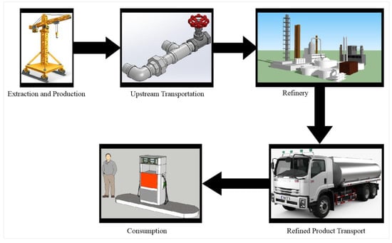
Figure 1.
Cycle of petroleum products.
- Extraction and production: After exploration, the site for drilling/mining is determined. Then, the process of extraction begins. This process is time-consuming and costly. Numerous measurements, experiments, sampling, drilling and boring wells are required to approve the existence of the natural resource. There are many obstacles in the said process, which are somewhat removed by modern machineries.
- Crude oil transportation: Crude oil needs to be transferred from wells to a refinery or storage facilities. After successful extraction of raw petroleum from the Earth, the best mode of transportation is determined. There are several factors influencing the means of transportation, such as geography, infrastructure and cost implications. Crude oil can be transported through various means, which are briefly described in Table 1. Since, pipelines are the most commonly used option to transport the crude oil, it is not only the cheapest but also a safe way for transporting petroleum from upstream to refinery and then from refinery to downstream. Thus, this application will consider the pipelines for the mathematical analysis.
 Table 1. Means of transportation of oil and gas.
 - Refinery: A refinery is an industrial plant that refines/transforms the crude oil into different pure and perfect energy products, which can be used as fuels, such as heating oils, gasoline, petrol and diesel. These refineries also serve as secondary storage for petroleum products.
- Refined product transport: Once the crude oil and raw petroleum is refined, the final and pure products are ready to be distributed. Therefore, the commodities are moved to their destined storages. The options of transport are similar to the upstream transportation. Natural gas uses pipelines and petrol/diesel are mostly moved by oil tankers.
- Consumption: Finally, the ultimate products are delivered to the consumers; i.e., filling stations, houses, factories, industries, etc. The consumers burn these resources to fulfill their energy requirements.
As we are now familiar with the complete cycle and all the stages of the process, it is convenient to discuss terrorist attacks. Table 2 gives the abbreviations and the mathematical values of these attacks for mathematical analysis. The assignation of the fuzzy values to these risk factors is an essential technique. In order to do so, the risks are deeply studied and the situations of different companies are carefully analyzed. Then, on the basis of these expert observations, each of the factors are assigned a value. These values describe different aspects of a factor. The proposed model is elegant and supple in that its numerical values can be representative of diverse characteristics. In this paper, the threat and hazard levels have been characterized by these values. Further explanations will be provided in the calculation sections.
Table 2.
Abbreviation and mathematical values for Terrorist attacks.
- a.
- Attack on Exploration Site
Explorations and developments are often sited in faraway areas, where communication to the authorities, transportation networks and related security setups are poor. Thus, it is difficult to stop an outside invasion. In the case of state-served security for shielding the site, attackers usually outnumber these forces, since these terrorists typically belong to the surrounding groups. These attacks also require relatively small amounts of explosives, which allows a single person to bring such things simultaneously. Thus, such sites are attractive targets for them. These terrorists can use vehicles, UAVs and speedboats. Thus, they are capable of performing organized attacks on these isolated locations.
These terrorists can possibly coordinate a wide range of attacks. Some possible attacks are listed below:
- Murder or kidnap the employees;
- Suicide attacks (vehicle bombs);
- Cover attacks;
- Destruction of pipelines;
- Destroying communication systems;
- Hijacking fuel carrying vehicles.
- b.
- Attack on Transport
Tankers are comparatively easy targets for the terrorists. They aim to attack ships at sea because of the following reasons:
- Limited onboard security countermeasures to discourage potential attackers such as high-powered sirens or pressured water hoses;
- The availability of security crew is reasonably low;
- The freight onboard is an ecologically harmful and inflammable product;
- The support accessible from external securities is only with extensive time delays.
- c.
- Attack on Refinery
In the cycle of petroleum fuels, a refinery is the most valuable asset. Its security is the utmost necessity for a continuous operation. The refining capacities are extended to the limits in numerous countries. The greatest security challenges for a refinery are due to the following reasons:
- Refinery covers a large area;
- Complex operations;
- Substantial flow of material and people, i.e., external contractors and staff.
The national authorities and managing crew of the refinery acknowledge its worth. Henceforth, they provide a number of security layers around it.
- d.
- Attack on Offshore Platform
The offshore platforms are part of the national framework of critical infrastructure. Hence, they are given greater physical security. However, a fighter ship with superior operational and technical capabilities cannot hold off a terrorist attack, and it is vulnerable to a suicide terrorist boat attack.
- e.
- Attack on Retailing Sector
When the final products are refined in the refinery from the crude oil, they are distributed to the trading sectors. Since these products are highly inflammable and hazardous; thus, they are the most vulnerable assets to attacks. Trucks and vehicles (railcars) carrying these fuels are visible in traffic flows. The attack against a stationary target is comparatively easier than performing an attack against a moving target, as these vehicles have many episodes of parking, loading and unloading, which lead to smooth attacks. Moreover, the sale and purchase points (storage region and filling stations) are physically insecure and are located in highly populated areas. Due to great population density and the explosive nature of gas and fuels, any terrorist attack might have major consequences. Henceforth, such weak (defenseless) points are attractive targets for attackers. Additionally, considering the risk of an ill use of trucks carrying fuel tanks, they could be used as an explosive weapon, which can easily destroy a building. The fire afterward will have additional consequences. Thus, there is high possibility of huge destruction.
4.3. Recommended Security Measures
As the petroleum industries face growing security threats and attacks, it is recommended to counter these threats by engaging in a two-pronged global initiative, i.e., merging the features of operational security and strategic security.
- Strategic Security
Terrorists are expected to organize strong tactical attacks, such as attacking a few components of the petroleum cycle and responding aggressively to security crew. Thus, all the assets of petroleum cycle (extraction to distribution) should be secured. It must be considered a national strategic concern. Some of the recommended physical security practices are discussed below:
- Make organizations stronger through government security agencies and first responders. For mathematical analysis, this strategy will be denoted by .
- Diminish the possibility of successful terrorist attack by advanced, technical and operational security methods. This strategy will be denoted by .
- In order to shrink the chances of terrorist attacks, carry out continuous security drills and exercises at all levels. This strategy will be symbolized by .
- In order to minimize the inside terrorizations and strengthen the company’s resilience, it is required to adopt the culture of corporate security. This strategy will be symbolized by for mathematical purposes.
- Update and evaluate the security tactics and strategies to counter the risks. Mathematically, it will be represented by .
- A regular assessment of risk and threat should be carried out in order to identify the risks in case of a changing environment. will be used to represent this strategy in calculations.
Similar to the construction rules of Table 2, Table 3 is constructed, which sets the security techniques and allocates them into certain fuzzy numbers. These fuzzy numbers are representatives of security and weakness levels. The values assigned to these securities greatly depend on the analysis of circumstances and expert observation of the securities in different scenarios. Based on these careful observations, the values are professionally assigned after being translated into fuzzy theory.
Table 3.
Mathematical values for security techniques.
- Operational Security
Currently, to minimize security threats and risks, major struggles are being made to achieve stronger assessment and security abilities:
- g.
- Development of high technology (denoted by ): Robotic helicopters, automatic weaponized UAVs, wrapping the pipelines with carbon fiber for protection, use of modern geographic and satellite monitoring data systems combined with sets of ground-based data for integrated 3D-vulnerability assessment, application of alarms with seismic sensors for providing instant warning to response teams.
- h.
- Logistics (denoted by ): Maintaining a sufficient inventory of custom-built replacement parts, shortening the repair time after an attack, solidification of physical security at serious interchanges, better physical access control, encrypted communication, layered and restricted access for reaching areas of a higher value, instantaneous monitoring of vehicle data.
- i.
- Training and Policy (denoted by OS3): Execution of industrial corporate security awareness programs for the development of a security policy, facilitating all the workers with security training and security strategies. Strategies to identify insider, global marketing, and communication of security as a defensive tool.
4.4. Fuzzy Mathematical Analysis
The algorithm for carrying out the proposed method is depicted in Figure 2.
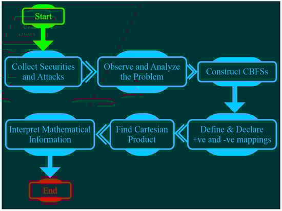
Figure 2.
Algorithm for the proposed method.
In order to perform a mathematical analysis based on the proposed methods, a set of securities and a set of terrorist attacks are constructed. In previous subsections, Table 2 and Table 3 describe the sets and , respectively. Additionally, the values of positive and negative membership mappings are also assigned. Hence,
In set , the values of positive membership mappings indicate the security levels, and the values of negative membership mappings indicate the weakness levels. Each value is represented by a complex number in an exponential form. The amplitude terms specify the partial membership of the elements to the set, i.e., the higher values of positive membership amplitude terms show that the security provided is strong and vice versa, whereas the higher value of negative membership amplitude terms show the weakness levels of security practices and vice versa. Moreover, the phase terms refer to the duration or time phase. Hence, these values describe the specifications of security with respect to the time phase. In case of positive values, the numbers closer to are considered high and those near are said to be low. In contrast, the negative membership values are higher when they are close to and lower when closer to .
Similar is the case with the set of attacks . The value of positive membership mapping of an attack represents the level of threat and strength of that attack with respect to some time frame. Conversely, the values of negative membership mapping characterize the level of danger, hazard or disaster that can happen due to those attacks. Again, the value of amplitude terms shows the strength and weakness of said properties that are possessed by an attack. The phase terms refer to time phase. The higher values of amplitude terms in positive membership mappings are signs of extreme attacks and vice versa, while the higher values of amplitude terms in negative membership mappings point toward the ability to achieve higher damage and destruction and vice versa. The rules of higher and lower values are the same as for the set of securities S.
Now, the Cartesian product is found to study the relationships of these attacks against the recommended security types. The Cartesian product is presented in Table 4, which is obtained by using Definition 8.
Table 4.
Cartesian product between the sets of securities and attacks: .
.
The above table shows the Cartesian product between the set of securities and the set of terrorist attacks . Both of the sets are CBFSs; thus, their Cartesian product is a CBFR. Each member of is in the form of a pair of elements. The first element in each pair belongs to the set of securities, and the second element belongs to the set of terrorist attacks. The relation between the elements of a pair is described through the numerical values, i.e., values of positive and negative membership mappings. Due to their complex nature, the values are complex numbers written in exponential form. The positive membership mapping represents the level of security provided by a particular security against a certain attack. For example, the pair tells the relations between security of high-tech development and the terrorist attack on a refinery. Its positive membership mapping takes values to mean the security level of high-tech development against an attack on a refinery, and the negative membership mapping explains the vulnerability of the said security system to other attacks after being attacked.
The amplitude term with the higher value (closer to ) of a positive membership mapping tells that the security level provided by the first element against the attack in the ordered pair is great, and the lower value of positive membership mapping (near ) shows that the security strategy cannot hold the particular attack. Alternatively, the amplitude term with higher value (close to ) of a negative membership mapping tells that the level of vulnerability of the security system, after being hit by a terrorist attack (mentioned in the order pair), is high, and the lower value of amplitude term of negative membership mapping (near ) shows that the exposure of that security system is low. The phase terms refer to the time phase. For better understanding, let us interpret the relation . The value of positive membership mapping tells that high-tech development provides higher security of or for half a month (in the case when the time phase is a month) against an attack of terrorists on an exploration site, whereas the value of negative membership puts forward that, after an attack on a refinery, the defending high-tech development system weakens up to for a 10th of a month, i.e., 3 days. In the same way, the numerical results of every relation can be interpreted.
The proposed modeling method provides a possible solution for security issues for the oil and gas industries. The authorities can think of several securities and assume different attack types. The proposed method has the capability of suggesting the best security strategy for particular sites against specific attacks. Furthermore, the repair time and the time of high alerts after an attack can be predicted. Conversely, a question arises on the validity of the results achieved by the proposed modeling method when they are applied to large data. The outcomes obtained in this article can be verified by an ample discussion and systematic analysis. In application, we only apply the proposed model to the data for the security problems faced by petroleum industries. In this case, if the data size increases, the proposed model is still applicable. Hence, the working of this model and solution methods are impeccable for any size of data. Moreover, the contribution of this research, particularly the models and the mathematical techniques, is to provide advantages to the industries and help them build a secure industrial system. The industries might provide a small amount of data, which can be manually manipulated using the proposed method. However, if an industry offers big data, then a computer-based program and algorithm will be required to carry out the operations to achieve the obligatory results.
The validity of the proposed methodology and given structures is experimentally shown in the coming section by a deep comparative study. Here, the practical world problems are analyzed carefully and modeled through fuzzy information. Initially, the information is converted to the fuzzy numerical form by standard methodology, as used by Zhang [19,20], Lee and Hur [24], Alkouri et al. [26] and Ref [31,32]. Then, for solving fuzzy information, the CBFSs and CBFRs are selected to fulfill the requirement of a strong fuzzy structure and tool. Next, we present the detailed comparison and head-to-head advantages of the selected model and structures in the following section.
5. Comparative Analysis
This section compares the proposed method with the other methods in the literature such as fuzzy sets, complex fuzzy sets and bipolar fuzzy sets. Each comparison is carried out in a separate section. For a fair match, the above application is solved using other methods and structures.
5.1. Comparison with Fuzzy Sets and Relations
According to Definition 1, the structure of an FS is composed of an element and an associated membership mapping. We define the two sets and , representing the securities and terrorist attacks, respectively.
In set , the values of membership mappings indicate the security levels. Each value is represented by a real number between and . The higher values of membership mappings show the higher levels of security being provided and vice versa. The numbers closer to are considered high, and those near are said to be low, since in the standard fuzzy modeling methods, the membership mappings can be set to represent some features of an entity. Henceforth, by following these regulations, the value of membership mapping of an attack in a set is used to characterize the level of threat and strength of that attack. The higher value of membership mapping points toward an extreme attack and vice versa.
Now, in an environment of FSs, the Cartesian product is found to study the relationships of these attacks against the recommended security types. The Cartesian product is presented in Table 5.
Table 5.
Cartesian product in a fuzzy environment.
Cartesian product between the set of securities and the set of terrorist attacks is given by the above table. The relation between the elements of a pair is described through the values of membership mappings. The membership mapping represents the level of security provided by a particular security against a certain attack. For example, tells the relations between security of “evaluation of security tactics” and the terrorist attack on an offshore platform. Its membership mapping value determines that the security level of the “evaluation of security tactics” against an attack on an offshore platform is .
Remark 1:
The modeling abilities of an FS are imperfect for the solution of the problem of interest because the structure of an FS lacks the negative membership mapping and uses the real valued fuzzy numbers. The major downsides are that FSs cannot represent the time phase and the level of vulnerability of a security.
5.2. Comparison with Bipolar Fuzzy Sets and Relations
Definition 5 states that the structure of a BFS includes an element that is assigned a couple of fuzzy numbers, known as positive membership mapping and negative membership mapping. Two sets and , representing the securities and terrorist attacks, respectively, are defined as
The values of positive membership mappings represent the security levels of securities in set . The values of negative membership mappings represent the weakness levels of that security system. The higher values of positive membership mappings (closer to ) show the higher levels of security being provided and vice versa. The higher values of negative membership mappings (closer to 0) show great weakness of security and vice versa.
The values of positive membership mappings represent the threat levels of terrorist attacks in set , and the values of negative membership mappings represent the destruction capacity of an attack.
To find out the relationships of attacks and the recommended security types in the environment of BFSs, the Cartesian product is found, which is given by Table 6.
Table 6.
Cartesian product in a bipolar fuzzy environment.
In the above table, the positive membership mapping represents the security level that a certain security provides against a specific attack. For example, translates as the security given by the “evaluation of security tactics” against a terrorist attack on an offshore platform is 62.5%, and this security system weakens up to after such an attack.
Remark 2:
Similar to FSs, the modeling abilities of BFS are also incomplete and do not give a detailed solution. The structure of BFSs does not carry complex valued mappings, which restricts it to a model of a single-variable problem. It provides some useful information such as the security levels and vulnerability of those securities but fails to discuss the time phase, which places the BFSs and relation back.
5.3. Comparison with Complex Fuzzy Sets and Relations
As stated by Definition 2, the elements of CFS are assigned a complex valued number, called the membership mapping. Let us construct the sets and of securities and terrorist attacks, respectively.
The membership mapping of security specifies the security levels with respect to time phase, since the values of membership mappings are complex numbers written in exponential form. Thus, each value has two parts: amplitude term refers to the level of security and the phase term refers to the time phase. The values of amplitude and phase term are considered higher when close to 1 and lower as they approach 0. The membership mapping of an attack in specifies the level of threat of that attack with respect to the time phase. The higher values are an indication of a dangerous attack and vice versa.
Now, the Cartesian product S × A is established in Table 7. It will be interpreted to analyze the relationships among the recommended security types and the terrorist attacks.
Table 7.
Cartesian product in a complex fuzzy environment.
Here, the elements of the Cartesian product have complex valued membership mappings. The relation between a security and an attack describes the level of security against a specific attack, which is designated by the membership mapping’s value. For example, expresses the relation between the security named, “evaluation of security tactics” and the terrorist attack on an offshore platform. The amplitude term’s value of membership mapping is , which states that the said security tactic can provide safety against an attack on an offshore platform. The phase term’s value is , which is equivalent to days (when the time phase is a month). Therefore, the relation infers that “evaluation of security tactics” has a capacity of coping with an “attack on refinery” up to days.
Remark 3:
The major drawback of CFSs and relations is the absence of negative membership mapping. Therefore, it is incapable of solving the problem of interest up to required standards. This concept does not specify the weakness of securities, vulnerability of security strategies after being hit by attackers, or the capacity of damage by an attack.
Different methods have resulted in different numerical values. Thus, it is difficult to compare these methods without any standard, which makes the ranking of these methods problematic. Therefore, a fundamental rule for the classification and ranking of fuzzy methods is generally based on the domain and range of that particular structure. In other words, the structure is considered to be superior if it consists of more mappings to represent different features and a greater domain and range of numerical values. In fuzzy theory, a superior structure always generalizes other inferior frameworks, which means that a better method has the ability to handle the information in several fuzzy frameworks. Now, by following these standards, some conclusive remarks for the above analysis are given below. To conclude this comparative analysis, Table 8 is constructed, which shows a head-to-head comparison among all these structures, including the proposed method.
Table 8.
A structural and technical comparison among different frameworks.
From Table 8, it is clear that the structure of CBFRs is the most powerful versus the others, and thus the proposed method that is based on CBFRs is the supreme modeling technique. All of the other methods have failed to produce the required results. The method initiated in this research develops some useful results. Future plans include programming and automated algorithms for the proposed methods. It will not only improve the practicality of the method, but it will also validate the outcomes of different methods.
6. Conclusions
In this article, a new concept of Cartesian product between complex bipolar fuzzy sets (CBFSs) was introduced. Moreover, the complex bipolar fuzzy relations (CBFR) were defined, which are based on the concept of the Cartesian product. These relations were used to study the relationships between two sets in the environments of complex bipolar fuzzy information, bipolar fuzzy information, complex fuzzy information and fuzzy information. Likewise, the complex bipolar fuzzy equivalence relation, complex bipolar fuzzy partial order relation, complex bipolar fuzzy linear order relation, complex bipolar fuzzy composite relation and numerous other types of CBFRs were defined with easy-to-follow examples. Further, the equivalence classes for complex bipolar fuzzy equivalence relation were also deliberated.
Additionally, the proposed methods were used to model the security issues that the petroleum industries encounter. Particularly, terrorist attacks and their counter measures were analyzed using CBFRs. Consequently, the proposed model and the analysis of security problems in the oil and gas sectors mathematically verified the efficiency of some security techniques. As a result, it is recommended to apply the combination of strategic securities and operational securities to tackle terrorist attacks and minimize their consequences. The advantage of using CBFRs is that it offers the ability to model time variables along with a variable of interest. Likewise, it also discusses the dual properties of an object. Furthermore, the proposed modeling technique was compared to other fuzzy modeling techniques. Thus, the proposed methods were confirmed to be more superior and efficient. In the future, the extended versions of the proposed methods will be formed that could produce some interesting structures. Further, the intelligent algorithms and programs would be generated for these structures to enrich their modeling capabilities, and thus, they will be more applicable.
Author Contributions
Conceptualization, A.N., N.J. and D.P.; methodology, A.N., N.J. and M.-S.Y.; software, A.N. and S.U.K.; validation, D.P. and D.M.; formal analysis, M.-S.Y., D.M. and S.U.K.; investigation, A.N., N.J., M.-S.Y. and D.P.; resources, D.M. and S.U.K.; data curation, A.N., N.J. and S.U.K.; writing—original draft preparation, A.N., N.J., and D.M.; writing—review and editing, N.J., M.-S.Y. and D.P.; visualization, D.P., D.M. and S.U.K.; supervision, M.-S.Y. and D.P.; project administration, A.N. and N.J.; funding acquisition, M.-S.Y. All authors have read and agreed to the published version of the manuscript.
Funding
This research was funded in part by the Ministry of Science and technology (MOST) of Taiwan under grant MOST-110-2118-M-033-003.
Data Availability Statement
Not applicable.
Conflicts of Interest
The authors declare no conflict of interest.
References
- Zadeh, L.A. Fuzzy sets. Inf. Control. 1965, 8, 338–353. [Google Scholar] [CrossRef] [Green Version]
- Kandel, A.; Byatt, W.J. Fuzzy sets, fuzzy algebra, and fuzzy statistics. Proc. IEEE 1978, 66, 1619–1639. [Google Scholar] [CrossRef]
- Robinson, V.B. A perspective on the fundamentals of fuzzy sets and their use in geographic information systems. Trans. GIS 2003, 7, 3–30. [Google Scholar] [CrossRef]
- Yang, M.S.; Hung, W.L.; Chang-Chien, S.J. On a similarity measure between LR-type fuzzy numbers and its application to database acquisition. Int. J. Intell. Syst. 2005, 20, 1001–1016. [Google Scholar] [CrossRef]
- Kabir, S.; Papadopoulos, Y. A review of applications of fuzzy sets to safety and reliability engineering. Int. J. Approx. Reason. 2018, 100, 29–55. [Google Scholar] [CrossRef]
- Mardani, A.; Hooker, R.E.; Ozkul, S.; Yifan, S.; Nilashi, M.; Sabzi, H.Z.; Fei, G.C. Application of decision making and fuzzy sets theory to evaluate the healthcare and medical problems: A review of three decades of research with recent developments. Expert Syst. Appl. 2019, 137, 202–231. [Google Scholar] [CrossRef]
- Mishra, A.R.; Rani, P.; Krishankumar, R.; Ravichandran, K.S.; Kar, S. An extended fuzzy decision-making framework using hesitant fuzzy sets for the drug selection to treat the mild symptoms of Coronavirus Disease 2019 (COVID-19). Appl. Soft Comput. 2021, 103, 107155. [Google Scholar] [CrossRef]
- Khalil, S.; Hassan, A.; Alaskar, H.; Khan, W.; Hussain, A. Fuzzy logical algebra and study of the effectiveness of medications for COVID-19. Mathematics 2021, 9, 2838. [Google Scholar] [CrossRef]
- Ramot, D.; Milo, R.; Friedman, M.; Kandel, A. Complex fuzzy sets. IEEE Trans Fuzzy Syst. 2002, 10, 171–186. [Google Scholar] [CrossRef]
- Ma, J.; Zhang, G.; Lu, J. A method for multiple periodic factor prediction problems using complex fuzzy sets. IEEE Trans. Fuzzy Syst. 2011, 20, 32–45. [Google Scholar]
- Tamura, S.; Higuchi, S.; Tanaka, K. Pattern classification based on fuzzy relations. IEEE Trans. Syst. Man Cybern. 1971, SMC-1, 61–66. [Google Scholar] [CrossRef] [Green Version]
- Yang, M.S.; Shih, H.M. Cluster analysis based on fuzzy relations. Fuzzy Sets Syst. 2001, 120, 197–212. [Google Scholar] [CrossRef]
- Ramot, D.; Friedman, M.; Langholz, G.; Kandel, A. Complex fuzzy logic. IEEE Trans. Fuzzy Syst. 2003, 11, 450–461. [Google Scholar] [CrossRef]
- Yazdanbakhsh, O.; Dick, S. A systematic review of complex fuzzy sets and logic. Fuzzy Sets Syst. 2018, 338, 1–22. [Google Scholar] [CrossRef]
- Ali, Z.; Mahmood, T.; Yang, M.S. TOPSIS method based on complex spherical fuzzy sets with Bonferroni mean operators. Mathematics 2020, 8, 1739. [Google Scholar] [CrossRef]
- Nasir, A.; Jan, N.; Gumaei, A.; Khan, S.U. Medical diagnosis and life span of sufferer using interval valued complex fuzzy relations. IEEE Access 2021, 9, 93764–93780. [Google Scholar] [CrossRef]
- Jan, N.; Nasir, A.; Alhilal, M.S.; Khan, S.U.; Pamucar, D.; Alothaim, A. Investigation of cyber-security and cyber-crimes in oil and gas sectors using the innovative structures of complex intuitionistic fuzzy relations. Entropy 2021, 23, 1112. [Google Scholar] [CrossRef]
- Nasir, A.; Jan, N.; Gumaei, A.; Khan, S.U.; Albogamy, F.R. Cybersecurity against the loopholes in industrial control systems using interval-valued complex intuitionistic fuzzy relations. Appl. Sci. 2021, 11, 7668. [Google Scholar] [CrossRef]
- Nasir, A.; Jan, N.; Gwak, J.; Khan, S.U. Investigation of financial track records by using some novel concepts of complex q-rung orthopair fuzzy information. IEEE Access 2021, 9, 152857–152877. [Google Scholar] [CrossRef]
- Zhang, W.R. Bipolar fuzzy sets and relations: A computational framework for cognitive modeling and multiagent decision analysis. In Proceedings of the First International Joint Conference of the North American Fuzzy Information Processing Society Biannual Conference, NAFIPS/IFIS/NASA’94, San Antonio, TX, USA, 18–21 December 1994; 1994; pp. 305–309. [Google Scholar]
- Zhang, W.R.; Zhang, L. YinYang bipolar logic and bipolar fuzzy logic. Inf. Sci. 2004, 165, 265–287. [Google Scholar] [CrossRef]
- Abdullah, S.; Aslam, M.; Ullah, K. Bipolar fuzzy soft sets and its applications in decision making problem. J. Intell. Fuzzy Syst. 2014, 27, 729–742. [Google Scholar] [CrossRef] [Green Version]
- Sarwar, M.; Akram, M. Bipolar fuzzy circuits with applications. J. Intell. Fuzzy Syst. 2018, 34, 547–558. [Google Scholar] [CrossRef]
- Akram, M.; Arshad, M. Bipolar fuzzy TOPSIS and bipolar fuzzy ELECTRE-I methods to diagnosis. Comput. Appl. Math. 2020, 39, 7. [Google Scholar] [CrossRef]
- Lee, J.G.; Hur, K. Bipolar fuzzy relations. Mathematics 2019, 7, 1044. [Google Scholar] [CrossRef] [Green Version]
- Ali, G.; Akram, M.; Alcantud, J.C.R. Attributes reductions of bipolar fuzzy relation decision systems. Neural Comput. Appl. 2020, 32, 10051–10071. [Google Scholar] [CrossRef]
- Alkouri, A.U.M.; Massa’deh, M.O.; Ali, M. On bipolar complex fuzzy sets and its application. J. Intell. Fuzzy Syst. 2020, 39, 383–397. [Google Scholar] [CrossRef]
- Akram, M.; Ali, M.; Allahviranloo, T. Solution of complex bipolar fuzzy linear system. In International Online Conference on Intelligent Decision Science; Springer: Cham, Switzerland, 2020; Volume 1301, pp. 899–927. [Google Scholar]
- Gulistan, M.; Yaqoob, N.; Elmoasry, A.; Alebraheem, J. Complex bipolar fuzzy sets: An application in a transport’s company. J. Intell. Fuzzy Syst. 2021, 40, 3981–3997. [Google Scholar] [CrossRef]
- Mahmood, T.; Rehman, U.U. A novel approach towards bipolar complex fuzzy sets and their applications in generalized similarity measures. Int. J. Intell. Syst. 2022, 37, 535–567. [Google Scholar] [CrossRef]
- Aliannezhadi, S.; Molai, A.A. A new algorithm for solving linear programming problems with bipolar fuzzy relation equation constraints. Iran. J. Numer. Anal. Optim. 2021, 11, 407–435. [Google Scholar]
- Dutta, P.; Doley, D. Medical diagnosis under uncertain environment through bipolar-valued fuzzy sets. In Computer Vision and Machine Intelligence in Medical Image Analysis; Springer: Singapore, 2020; pp. 127–135. [Google Scholar]
- Oil, Terrorism and Drugs Intermingle in Colombia. IAGS Energy Security. 5 August 2003. Available online: http://www.iags.org/n0805032.htm (accessed on 22 January 2022).
- Luft, G. Pipeline sabotage is terrorist’s weapon of choice. Pipeline Gas J. 2005, 232, 42–44. [Google Scholar]
Publisher’s Note: MDPI stays neutral with regard to jurisdictional claims in published maps and institutional affiliations. |
© 2022 by the authors. Licensee MDPI, Basel, Switzerland. This article is an open access article distributed under the terms and conditions of the Creative Commons Attribution (CC BY) license (https://creativecommons.org/licenses/by/4.0/).