
Stochastic Triad Topology Based Particle Swarm Optimization for Global Numerical Optimization

 ,
, 
Abstract
1. Introduction
- (1)
- A stochastic triad topology is employed to connect the personal best position of each particle and two different personal best positions randomly selected from those of the rest particles to select guiding exemplars for particles to update. Different from existing studies [22,37], which only utilize the topologies to determine the best position to replace the social exemplar, namely gbest, in the classical PSO (with another guiding exemplar as the personal best position of the particle), the proposed STTPSO utilizes the stochastic triad topology to select the best one and computes the mean position of the triad best positions as the two guiding exemplars to direct the update of each particle. Since the topology is stochastic, it is likely that different particles preserve different guiding exemplars. As a result, the learning diversity of particles can be largely promoted, and thus the probability of the swarm escaping from local areas can be promoted.
- (2)
- An archive is maintained to store the obsolete personal best positions and then is combined with the personal best positions of all particles in the current generation to form the triad topologies for particles. In this way, valuable historical information can be utilized to direct the update of particles, which is helpful for improving swarm diversity.
- (3)
- A random restart strategy is designed by randomly initializing a solution with a small probability. However, instead of employing this restart strategy on the swarm, we utilize it on the archive. That is to say, a randomly initialized solution is inserted into the archive with a small probability. In this way, the swarm diversity can be promoted without significant sacrifice of convergence speed.
- (4)
- A dynamic strategy for the acceleration coefficients is devised to alleviate the sensitivity of STTPSO. Instead of utilizing fixed values for the two acceleration coefficients, this paper randomly samples the two acceleration coefficients based on the Gaussian distribution with the mean value set as the classical setting of the two coefficients and a small deviation. With this dynamic strategy, different particles can have different settings, and thus the learning diversity can be further promoted.
2. Related Works
2.1. Basic PSO
2.2. Advanced Learning Strategies for PSO

| Category | Methods | Characteristics | ||
|---|---|---|---|---|
| Topology-based Methods | Static Topology | Full Topology | PSO [6,7] | Each particle can only communicate with fixed peers. The learning diversity of particles is limited. |
| Ring Topology | MRTPSO [26], GGL-PSOD [56] | |||
| Pyramid Topology | PMKPSO [27] | |||
| Star Topology | PSO-Star [29,55] | |||
| Von Neumann Topology | PSO-Von-Neumann [29] | |||
| Hybrid Topology | XPSO [23] | |||
| Dynamic Topology | Dynamic Topology | DNSPSO [28], DMSPSO [15], SPSO [22] | Each particle communicates with dynamic peers. The learning diversity of particles is high. | |
| Dynamic Size Topology | RPSO [16] | |||
| Exemplar construction-based Methods | Random Construction | CLPSO_LS [14], CLPSO [17], HCLPSO [25], TCSPSO [19] | Randomly recombine dimensions of personal best positions. The exemplar construction efficiency is low, but it consumes no fitness evaluations in exemplar construction. | |
| Operator-based Construction | MPSOEG [24], GLPSO [18] | Recombine dimensions of personal best positions based evolutionary operators in other EAs. The exemplar construction efficiency is high, but it consumes many fitness evaluations in exemplar construction | ||
| Orthogonal Recombination | OLPSO [37] | Recombine dimensions of personal best positions based on orthogonal experimental design. The exemplar construction efficiency is high, but it consumes a lot of fitness evaluation in exemplar construction | ||
3. Stochastic Triad Topology-Based Particle Swarm Optimization
3.1. Stochastic Triad Topology
Remark
- (1)
- Unlike existing studies that use the random topologies to determine only one guiding exemplar to replace the social exemplar (gbest) in the classical PSO [6,7], the proposed STTPSO utilizes the stochastic triad topology for each particle to select the best one among the triad personal best positions and computes the mean position of these pbests as the two guiding exemplars to direct the update of this particle. In this way, due to the randomness of the triad topology, not only the diversity of the first exemplar is promoted largely, but also the diversity of the second exemplar is promoted to a large extent. Therefore, the learning diversity of particles is improved, which is beneficial for enhancing the chance of escaping from local areas for the swarm.
- (2)
- Unlike existing studies that change the random topology structure every generation, this paper adaptively changes the triad topology structure based on the evolution state of each particle. In particular, we record stagnation times of each particle (xi), which is actually the number of continuous generations where the personal best position (pbesti) of the particle remains unchanged. When such a number exceeds a predefined threshold stopmax, the triad topology structure is reconstructed by randomly reselecting two different personal best positions from those of other particles. In this way, the triad topology structure of each particle is changed asynchronously, which guarantees the learning effectiveness of particles.
3.2. Dynamic Acceleration Coefficients
3.3. Historical Information Utilization
3.4. Random Restart Strategy
3.5. Overall Procedure
| Algorithm 1: The pseudocode of STTPSO |
| Input: swarm size PS, maximum fitness evaluations FEmax, maximum stagnation times stopmax, restart probability pm; |
| 1: Initialize PS particles randomly and calculate their fitness; |
| 2: Set fes = PS, and set the archive empty; |
| 3: Randomly select two different personal best positions (pbestr1 and pbestr2) from the personal best positions of |
| other particles and the archive for each particle to form the associated triad topology; |
| 4: Set the stagnation time stopi = 0 (1 ≤ i ≤ PS) for each particle; |
| 5: While (fes ≤ FEmax) do |
| 6: For i = 1:PS do |
| 7: Compute w according to Equation (3); |
| 8: Randomly sample c1 and c2 from Gaussian(1.49618,0.1); |
| 9: If c1 < c2 then |
| 10: Swap c1 and c2; |
| 11: End If |
| 12: Update xi and vi according to Equations (2) and (4); |
| 13: Calculate the fitness of the updated xi: f(xi) and fes + = 1; |
| 14: If f(xi) < f(pbesti) then |
| 15: Put pbesti in the archive and set stopi = 0; |
| 16: pbesti = xi; |
| 17: Else |
| 18: stopi += 1; |
| 19: End If |
| 20: If stopi >= stopmax then |
| Reselect two different personal best positions (pbestr1 and pbestr2) from those of other particles and |
| 21: the archive for xi to form the associated triad topology; |
| 22: End If |
| 23: End For |
| 24: If rand(0, 1) < pm then |
| 25: Randomly initialize a solution and store it into the archive; |
| 26: End If |
| 27: End While |
| 28: Obtain the global best solution gbest and its fitness f(gbest); |
| Output: f(gbest) and gbest |
4. Experiments
4.1. Experimental Setup
4.2. Comparison with State-of-the-Art PSO Variants
- (1)
- According to the Friedman test results as shown in the last row, STTPSO achieves the lowest rank among all eight algorithms and its rank value (1.86) is much smaller than those (at least 2.55) of the seven compared algorithms. This demonstrates that STTPSO achieves the best overall performance on the 30-D CEC 2017 benchmark functions, and presents significant superiority over the seven compared algorithms.
- (2)
- The second last row of Table 2 shows that STTPSO is significantly superior to the compared algorithms on at least 21 problems except for XPSO, and only presents inferior performance on, at most, five problems. Compared with XPSO, STTPSO obtains significantly better performance on 18 problems, while only performing worse than XPSO on three problems.
- (3)
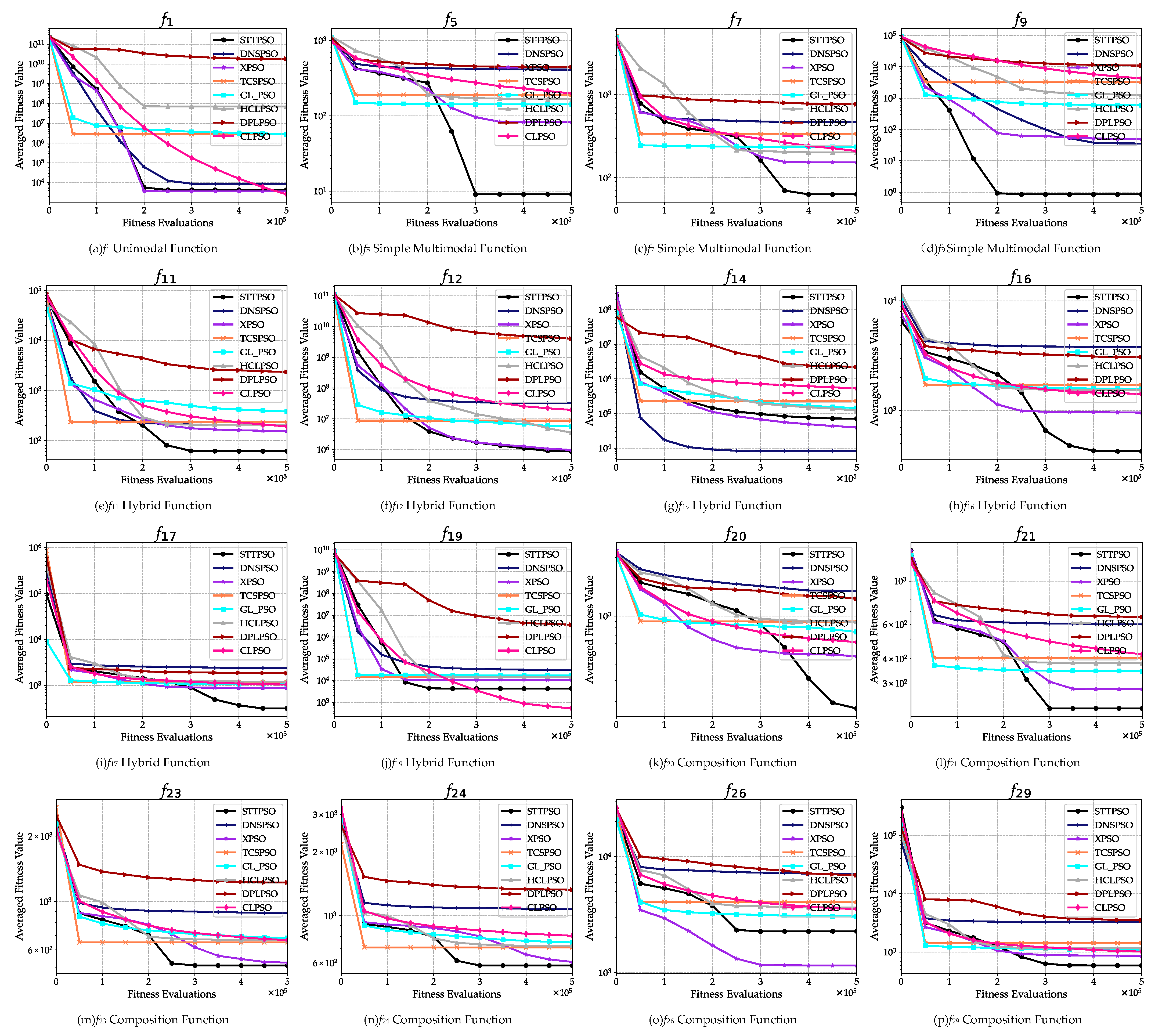
- In terms of the comparison results on different types of optimization problems, STTPSO achieves highly competitive performance with all the compared algorithms on the two unimodal problems. In particular, it shows significant dominance to DNSPSO and DPLPSO both on the two problems. In terms of the six simple multimodal problems, except for DNSPSO, STTPSO shows significantly better performance than the other six compared algorithms on all these problems. Compared with DNSPSO, STTPSO presents significant superiority on five problems and shows inferiority on only one problem. Regarding the 10 hybrid problems, STTPSO shows much better performance than DPLPSO on all 10 problems. Compared with DNSPSO, TCSPSO, and HCLPSO, STTPSO obtains significantly better performance on seven, six, and seven problems, respectively, and only shows inferiority to them on, at most, two problems. In comparison with XPSO, GLPSO, and CLPSO, STTPSO achieves no worse performance on at least seven problems and displays inferiority to them on, at most, three problems. Concerning the 11 composition problems, STTPSO outperforms the seven compared algorithms on at least nine problems, and only shows inferiority on, at most, two problems. In particular, STTPSO significantly outperforms both TCSPSO and GLPSO on all these problems and obtains much better performance than both HCLPSO and DPLPSO on 10 problems with no inferiority to them on all the 11 problems. Overall, it is demonstrated that STTPSO shows promise in solving various kinds of problems and particularly obtains good performance on complicated problems, such as multimodal problems, hybrid problems, and composition problems.
- (1)
- According to the Friedman test results shown in the last row, STTPSO achieves the lowest rank. This indicates that STTPSO still achieves the best overall performance on the whole 50-D CEC 2017 benchmark set. In particular, except for XPSO, its rank value (2.17) is much smaller than those (at least 4.14) of the other six compared algorithms. This demonstrates that STTPSO displays significantly better overall performance than the six compared algorithms.
- (2)
- From the perspective of the Wilcoxon rank sum test, as shown in the second to last row, STTPSO achieves significantly better performance than the seven compared algorithms on at least 19 problems and shows inferiority to them on, at most, five problems. In particular, compared with DNSPSO, TCSPSO, GLPSO, and CLPSO, STTPSO significantly dominates them all on 23 problems. In comparison with DPLPSO, STTPSO presents significant superiority on all the 29 problems.
- (3)
- In terms of different types of optimization problems, STTPSO achieves highly competitive performance with the seven compared state-of-the-art PSO variants regarding the two unimodal problems. Particularly, STTPSO defeats DPLPSO concerning these two problems. On the six simple multimodal problems, STTPSO performs much better than the seven compared algorithms on at least five problems. In particular, STTPSO presents significant dominance to XPSO, TCSPSO, GLPSO, DPLPSO, and CLPSO on all the six problems. Regarding the 10 hybrid problems, except for XPSO, STTPSO is significantly superior to the seven compared algorithms on at least seven problems, and shows inferiority on, at most, three problems. In particular, STTPSO significantly outperforms DPLPSO on all the 10 problems and obtains significantly better performance than DNSPSO on nine problems. Concerning the 11 composition problems, STTPSO displays significantly better performance than the seven state-of-the-art PSO variants on at least eight problems, and performs worse than them on, at most, two problems. Particularly, STTPSO shows significant dominance to DPLPSO on all the 11 problems and obtains much better performance than both TCSPSO and GLPSO on 10 problems. Overall, it is still demonstrated that STTPSO is a promising approach for problem optimization and displays its sound optimization ability in solving complicated optimization problems, such as multimodal problems, hybrid problems, and composition problems.
- (1)
- According to the Friedman test results, STTPSO achieves the lowest rank among all algorithms. This verifies that STTPSO still obtains the best overall performance on the 100-D CEC 2017 benchmark set. In particular, its rank value (1.52) is much smaller than those (at least 2.72) of the seven compared algorithms. This further demonstrates that STTPSO displays significant dominance to the seven compared algorithms. Together with the observations on the 30-D and 50-D CEC 2017 benchmark set, we can see that STTPSO consistently performs the best on the CEC 2017 benchmark set with different dimension sizes among all eight algorithms, and consistently presents its significant superiority to the seven compared algorithms on the benchmark set with the three dimension sizes. Therefore, it is demonstrated that STTPSO preserves a good scalability to solve optimization problems.
- (2)
- Regarding the Wilcoxon rank sum test, from the second to last row, it is observed that STTPSO achieves significantly better performance than the seven compared algorithms on at least 20 problems and shows inferiority to them on, at most, four problems. In particular, STTPSO outperforms DPLPSO significantly on all the 29 problems, and obtains much better performance than TCSPSO, GLPSO, HCLPSO, and CLPSO on 24, 24, 26, and 27 problems, respectively.
- (3)
- With respect to the optimization performance on different types of optimization problems, STTPSO obtains highly competitive or even much better performance than the seven compared algorithms on the two unimodal problems. Particularly, STTPSO shows significant dominance to DPLPSO and CLPSO on the two problems. As for the six simple multimodal problems, except for DNSPSO, STTPSO exhibits significant superiority to the other six compared algorithms on all these six problems. Competed with DNSPSO, STTPSO also shows much better performance on five problems. In terms of the 10 hybrid problems, except for XPSO, STTPSO is significantly superior to the other six compared algorithms on at least seven problems. Compared with XPSO, STTPSO illustrates significantly better performance on five problems and does not show inferiority on any of the problems. In particular, it is discovered that STTPSO is significantly better than HCLPSO and DPLPSO on all the 10 problems. Regarding the 11 composition problems, except for DNSPSO, STTPSO achieves much better performance than the other six compared algorithms on at least nine problems. Compared with DNSPSO, it still performs much better on seven problems. Particularly, STTPSO shows significant superiority to DPLPSO on all the 11 problems, and obtains much better performance than TCSPSO, GLPSO, and CLPSO on 10 problems and shows no inferiority to the three compared methods on these kinds of problems. Overall, it is demonstrated that STTPSO is still effective at solving optimization problems, especially complicated problems, such as multimodal problems, hybrid problems, and composition problems.
4.3. Deep Investigation on STTPSO
4.3.1. Effectiveness of the Reformulation of the Stochastic Triad Topology
4.3.2. Effectiveness of the Additional Archive and the Proposed Random Restart Strategy
4.3.3. Effectiveness of the Dynamic Acceleration Coefficients
5. Conclusions
Author Contributions
Funding
Conflicts of Interest
References
- Li, L.; Chang, L.; Gu, T.; Sheng, W.; Wang, W. On the Norm of Dominant Difference for Many-Objective Particle Swarm Optimization. IEEE Trans. Cybern. 2021, 51, 2055–2067. [Google Scholar] [CrossRef] [PubMed]
- Xia, X.; Gui, L.; Yu, F.; Wu, H.; Wei, B.; Zhang, Y.L.; Zhan, Z.H. Triple Archives Particle Swarm Optimization. IEEE Trans. Cybern. 2020, 50, 4862–4875. [Google Scholar] [CrossRef] [PubMed]
- Liu, W.; Wang, Z.; Yuan, Y.; Zeng, N.; Hone, K.; Liu, X. A Novel Sigmoid-Function-Based Adaptive Weighted Particle Swarm Optimizer. IEEE Trans. Cybern. 2021, 51, 1085–1093. [Google Scholar] [CrossRef] [PubMed]
- Yang, Q.; Hua, L.; Gao, X.; Xu, D.; Lu, Z.; Jeon, S.-W.; Zhang, J. Stochastic Cognitive Dominance Leading Particle Swarm Optimization for Multimodal Problems. Mathematics 2022, 10, 761. [Google Scholar] [CrossRef]
- Yang, Q.; Chen, W.-N.; Zhang, J. Probabilistic Multimodal Optimization. In Metaheuristics for Finding Multiple Solutions; Springer: Berlin/Heidelberg, Germany, 2021; pp. 191–228. [Google Scholar]
- Eberhart, R.; Kennedy, J. A New Optimizer Using Particle Swarm Theory. In Proceedings of the International Symposium on Micro Machine and Human Science, Nagoya, Japan, 4–6 October 1995; pp. 39–43. [Google Scholar]
- Shi, Y.; Eberhart, R.C. Empirical Study of Particle Swarm Optimization. In Proceedings of the Congress on Evolutionary Computation, Washington, DC, USA, 6–9 July 1999; pp. 1945–1950. [Google Scholar]
- Tsekouras, G.E.; Tsimikas, J.; Kalloniatis, C.; Gritzalis, S. Interpretability Constraints for Fuzzy Modeling Implemented by Constrained Particle Swarm Optimization. IEEE Trans. Fuzzy Syst. 2018, 26, 2348–2361. [Google Scholar] [CrossRef]
- Lin, C.; Chen, C.; Lin, C. Efficient Self-Evolving Evolutionary Learning for Neurofuzzy Inference Systems. IEEE Trans. Fuzzy Syst. 2008, 16, 1476–1490. [Google Scholar]
- Yang, Q.; Chen, W.N.; Gu, T.; Jin, H.; Mao, W.; Zhang, J. An Adaptive Stochastic Dominant Learning Swarm Optimizer for High-Dimensional Optimization. IEEE Trans. Cybern. 2022, 52, 1960–1976. [Google Scholar] [CrossRef]
- Zhang, X.; Du, K.J.; Zhan, Z.H.; Kwong, S.; Gu, T.L.; Zhang, J. Cooperative Coevolutionary Bare-Bones Particle Swarm Optimization with Function Independent Decomposition for Large-Scale Supply Chain Network Design with Uncertainties. IEEE Trans. Cybern. 2020, 50, 4454–4468. [Google Scholar] [CrossRef]
- Chen, W.N.; Tan, D.Z.; Yang, Q.; Gu, T.; Zhang, J. Ant Colony Optimization for the Control of Pollutant Spreading on Social Networks. IEEE Trans. Cybern. 2020, 50, 4053–4065. [Google Scholar] [CrossRef]
- Ge, Q.; Guo, C.; Jiang, H.; Lu, Z.; Yao, G.; Zhang, J.; Hua, Q. Industrial Power Load Forecasting Method Based on Reinforcement Learning and PSO-LSSVM. IEEE Trans. Cybern. 2022, 52, 1112–1124. [Google Scholar] [CrossRef]
- Cao, Y.; Zhang, H.; Li, W.; Zhou, M.; Zhang, Y.; Chaovalitwongse, W.A. Comprehensive Learning Particle Swarm Optimization Algorithm With Local Search for Multimodal Functions. IEEE Trans. Evol. Comput. 2019, 23, 718–731. [Google Scholar] [CrossRef]
- Liang, J.J.; Suganthan, P.N. Dynamic Multi-swarm Particle Swarm Optimizer. In Proceedings of the IEEE Swarm Intelligence Symposium, Pasadena, CA, USA, 8–10 June 2005; pp. 124–129. [Google Scholar]
- Mirjalili, S.; Lewis, A. Obstacles and Difficulties for Robust Benchmark Problems: A Novel Penalty-based Robust Optimisation Method. Inf. Sci. 2016, 328, 485–509. [Google Scholar] [CrossRef]
- Liang, J.J.; Qin, A.K.; Suganthan, P.N.; Baskar, S. Comprehensive Learning Particle Swarm Optimizer for Global Optimization of Multimodal Functions. IEEE Trans. Evol. Comput. 2006, 10, 281–295. [Google Scholar] [CrossRef]
- Gong, Y.-J.; Li, J.-J.; Zhou, Y.; Li, Y.; Chung, H.S.-H.; Shi, Y.-H.; Zhang, J. Genetic Learning Particle Swarm Optimization. IEEE Trans. Cybern. 2015, 46, 2277–2290. [Google Scholar] [CrossRef] [PubMed]
- Zhang, X.; Liu, H.; Zhang, T.; Wang, Q.; Wang, Y.; Tu, L. Terminal Crossover and Steering-based Particle Swarm Optimization Algorithm with Disturbance. Appl. Soft Comput. 2019, 85, 105841. [Google Scholar] [CrossRef]
- Liu, Z.; Nishi, T. Strategy Dynamics Particle Swarm Optimizer. Inf. Sci. 2022, 582, 665–703. [Google Scholar] [CrossRef]
- Kennedy, J.; Mendes, R. Population Structure and Particle Swarm Performance. In Proceedings of the Congress on Evolutionary Computation, Honolulu, HI, USA, 12–17 May 2002; pp. 1671–1676. [Google Scholar]
- Clerc, M. Beyond Standard Particle Swarm Optimisation. Int. J. Swarm Intell. Res. 2010, 1. [Google Scholar] [CrossRef]
- Xia, X.; Gui, L.; He, G.; Wei, B.; Zhang, Y.; Yu, F.; Wu, H.; Zhan, Z.-H. An Expanded Particle Swarm Optimization Based on Multi-exemplar and Forgetting Ability. Inf. Sci. 2020, 508, 105–120. [Google Scholar] [CrossRef]
- Karim, A.A.; Isa, N.A.M.; Lim, W.H. Modified Particle Swarm Optimization with Effective Guides. IEEE Access 2020, 8, 188699–188725. [Google Scholar] [CrossRef]
- Lynn, N.; Suganthan, P.N. Heterogeneous Comprehensive Learning Particle Swarm Optimization with Enhanced Exploration and Exploitation. Swarm Evol. Comput. 2015, 24, 11–24. [Google Scholar] [CrossRef]
- Yue, C.; Qu, B.; Liang, J. A Multiobjective Particle Swarm Optimizer Using Ring Topology for Solving Multimodal Multiobjective Problems. IEEE Trans. Evol. Comput. 2018, 22, 805–817. [Google Scholar] [CrossRef]
- Chakraborty, A.; Ray, K.S.; Dutta, S.; Bhattacharyya, S.; Kolya, A. Species Inspired PSO based Pyramid Match Kernel Model (PMK) for Moving Object Motion Tracking. In Proceedings of the Fourth International Conference on Research in Computational Intelligence and Communication Networks, Kolkata, India, 22–23 November 2018; pp. 152–157. [Google Scholar]
- Nianyin, Z.; Zidong, W.; Weibo, L.; Hong, Z.; Kate, H.; Xiaohui, L. A Dynamic Neighborhood-based Switching Particle Swarm Optimization Algorithm. IEEE Trans. Cybern. 2020, 8, 701–717. [Google Scholar]
- Vazquez, J.C.; Valdez, F. Fuzzy Logic for Dynamic Adaptation in PSO with Multiple Topologies. In Proceedings of the 2013 Joint IFSA World Congress and NAFIPS Annual Meeting, Edmonton, AB, Canada, 24–28 June 2013; pp. 1197–1202. [Google Scholar]
- Liu, Q.; Wei, W.; Yuan, H.; Zhan, Z.-H.; Li, Y. Topology Selection for Particle Swarm Optimization. Inf. Sci. 2016, 363, 154–173. [Google Scholar] [CrossRef]
- Lin, W.; Bo, Y.; Jeff, O. Particle Swarm Optimization Using Dynamic Tournament Yopology. Appl. Soft Comput. 2016, 48, 584–596. [Google Scholar]
- Xia, X.; Gui, L.; Zhan, Z.-H. A Multi-swarm Particle Swarm Optimization Algorithm based on Dynamical Topology and Purposeful Detecting. Appl. Soft Comput. 2018, 67, 126–140. [Google Scholar] [CrossRef]
- Zou, J.; Deng, Q.; Zheng, J.; Yang, S. A Close Neighbor Mobility Method Using Particle Swarm Optimizer for Solving Multimodal Optimization Problems. Inf. Sci. 2020, 519, 332–347. [Google Scholar] [CrossRef]
- Parrott, D.; Xiaodong, L. Locating and Tracking Multiple Dynamic Optima by a Particle Swarm Model Using Speciation. IEEE Trans. Evol. Comput. 2006, 10, 440–458. [Google Scholar] [CrossRef]
- Cervantes, A.; Galvan, I.M.; Isasi, P. AMPSO: A New Particle Swarm Method for Nearest Neighborhood Classification. IEEE Trans. Syst. Man Cybern. Part B Cybern. 2009, 39, 1082–1091. [Google Scholar] [CrossRef]
- Janson, S.; Middendorf, M. A Hierarchical Particle Swarm Optimizer and Its Adaptive Variant. IEEE Trans. Syst. Man Cybern. Part B Cybern. 2005, 35, 1272–1282. [Google Scholar] [CrossRef]
- Zhan, Z.; Zhang, J.; Li, Y.; Shi, Y. Orthogonal Learning Particle Swarm Optimization. IEEE Trans. Evol. Comput. 2011, 15, 832–847. [Google Scholar] [CrossRef]
- Chen, S.; Hong, X.; Harris, C.J. Particle Swarm Optimization Aided Orthogonal Forward Regression for Unified Data Modeling. IEEE Trans. Evol. Comput. 2010, 14, 477–499. [Google Scholar] [CrossRef]
- Yang, Q.; Chen, W.N.; Yu, Z.; Gu, T.; Li, Y.; Zhang, H.; Zhang, J. Adaptive Multimodal Continuous Ant Colony Optimization. IEEE Trans. Evol. Comput. 2017, 21, 191–205. [Google Scholar] [CrossRef]
- Yang, Q.; Chen, W.N.; Li, Y.; Chen, C.L.P.; Xu, X.M.; Zhang, J. Multimodal Estimation of Distribution Algorithms. IEEE Trans. Cybern. 2017, 47, 636–650. [Google Scholar] [CrossRef] [PubMed]
- Yang, Q.; Li, Y.; Gao, X.-D.; Ma, Y.-Y.; Lu, Z.-Y.; Jeon, S.-W.; Zhang, J. An Adaptive Covariance Scaling Estimation of Distribution Algorithm. Mathematics 2021, 9, 3207. [Google Scholar] [CrossRef]
- Wei, F.F.; Chen, W.N.; Yang, Q.; Deng, J.; Zhang, J. A Classifier-Assisted Level-Based Learning Swarm Optimizer for Expensive Optimization. IEEE Trans. Evol. Comput. 2020, 25, 219–233. [Google Scholar] [CrossRef]
- Yang, Q.; Chen, W.N.; Gu, T.; Zhang, H.; Yuan, H.; Kwong, S.; Zhang, J. A Distributed Swarm Optimizer with Adaptive Communication for Large-Scale Optimization. IEEE Trans. Cybern. 2020, 50, 3393–3408. [Google Scholar] [CrossRef]
- Wu, G.; Mallipeddi, R.; Suganthan, P.N. Problem Definitions and Evaluation Criteria for The CEC 2017 Competition on Constrained Real-Parameter Optimization; Technical Report; National University of Defense Technology: Changsha, China; Kyungpook National University: Daegu, Korea; Nanyang Technological University: Singapore, 2017; pp. 1–16. [Google Scholar]
- Shen, Y.; Wei, L.; Zeng, C.; Chen, J. Particle Swarm Optimization with Double Learning Patterns. Comput. Intell. Neurosci. 2016, 2016, 6510303. [Google Scholar] [CrossRef]
- Xie, H.-Y.; Yang, Q.; Hu, X.-M.; Chen, W.N. Cross-generation Elites Guided Particle Swarm Optimization for large scale optimization. In Proceedings of the IEEE Symposium Series on Computational Intelligence, Athens, Greece, 6–9 December 2016; pp. 1–8. [Google Scholar]
- Yang, Q.; Chen, W.N.; Gu, T.; Zhang, H.; Deng, J.D.; Li, Y.; Zhang, J. Segment-Based Predominant Learning Swarm Optimizer for Large-Scale Optimization. IEEE Trans. Cybern. 2017, 47, 2896–2910. [Google Scholar] [CrossRef]
- Hesam, V.; Naser, S.H.; Mahsa, S. A Hybrid Generalized Reduced Gradient-based Particle Swarm Optimizer for Constrained Engineering Optimization Problems. J. Comput. Civ. Eng. 2021, 5, 86–119. [Google Scholar]
- Riaan, B.; Engelbrecht, A.P.; van den Bergh, F. A Niching Particle Swarm Optimizer. In Proceedings of the Asia-Pacific Conference on Simulated Evolution and Learning, Orchid Country Club, Singapore, 18–22 November 2002; pp. 692–696. [Google Scholar]
- Yousri, D.; Thanikanti, S.B.; Allam, D.; Ramachandaramurthy, V.K.; Eteiba, M.B. Fractional Chaotic Ensemble Particle Swarm Optimizer for Identifying the Single, Double, and Three Diode Photovoltaic Models’ Parameters. Energy 2020, 195, 116979. [Google Scholar] [CrossRef]
- Chen, X.; Tianfield, H.; Du, W. Bee-foraging Learning Particle SwarmOptimization. Appl. Soft Comput. 2021, 102, 107134. [Google Scholar] [CrossRef]
- Zhan, Z.-H.; Shi, L.; Tan, K.C.; Zhang, J. A Survey on Evolutionary Computation for Complex Continuous optimization. Artif. Intell. Rev. 2021, 55, 59–110. [Google Scholar] [CrossRef]
- Tao, X.; Li, X.; Chen, W.; Liang, T.; Qi, L. Self-Adaptive Two Roles Hybrid Learning Strategies-based Particle Swarm Optimization. Inf. Sci. 2021, 578. [Google Scholar] [CrossRef]
- Xu, G.; Zhao, X.; Wu, T.; Li, R.; Li, X. An Elitist Learning Particle Swarm Optimization with Scaling Mutation and Ring Topology. IEEE Access 2018, 6, 78453–78470. [Google Scholar] [CrossRef]
- Kennedy, J. Small Worlds and Mega-minds: Effects of Neighborhood Topology on Particle Swarm Performance. In Proceedings of the Congress on Evolutionary Computation, Washington, DC, USA, 6–9 July 1999; Volume 1933, pp. 1931–1938. [Google Scholar]
- Lin, A.; Sun, W.; Yu, H.; Wu, G.; Tang, H. Global Genetic Learning Particle Swarm Optimization with Diversity Enhancement by Ring Topology. Swarm Evol. Comput. 2019, 44, 571–583. [Google Scholar] [CrossRef]
- Turkey, M.; Poli, R. A Model for Analysing the Collective Dynamic Behaviour and Characterising the Exploitation of Population-Based Algorithms. Evol. Comput. 2014, 22, 159–188. [Google Scholar] [CrossRef]
- Zhang, J.; Sanderson, A.C. JADE: Adaptive Differential Evolution with Optional External Archive. IEEE Trans. Evol. Comput. 2009, 13, 945–958. [Google Scholar] [CrossRef]
- Djellali, H.; Ghoualmi, N. Improved Chaotic Initialization of Particle Swarm applied to Feature Selection. In Proceedings of the International Conference on Networking and Advanced Systems, Annaba, Algeria, 26–27 June 2019; pp. 1–5. [Google Scholar]
- Watanabe, M.; Ihara, K.; Kato, S.; Sakuma, T. Initialization Effects for PSO Based Storage Assignment Optimization. In Proceedings of the Global Conference on Consumer Electronics, Kyoto, Japan, 12–15 October 2021; pp. 494–495. [Google Scholar]
- Wang, C.J.; Fang, H.; Wang, C.; Daneshmand, M.; Wang, H. A Novel Initialization Method for Particle Swarm Optimization-based FCM in Big Biomedical Data. In Proceedings of the IEEE International Conference on Big Data, Santa Clara, CA, USA, 29 October–1 November 2015; pp. 2942–2944. [Google Scholar]
- Farooq, M.U.; Ahmad, A.; Hameed, A. Opposition-based Initialization and A Modified Pattern for Lnertia Weight (IW) in PSO. In Proceedings of the IEEE International Conference on INnovations in Intelligent SysTems and Applications, Gdynia, Poland, 3–5 July 2017; pp. 96–101. [Google Scholar]
- Guo, J.; Tang, S. An Improved Particle Swarm Optimization with Re-initialization Mechanism. In Proceedings of the International Conference on Intelligent Human-Machine Systems and Cybernetics, Hangzhou, China, 26–27 August 2009; pp. 437–441. [Google Scholar]

| Algorithm | D | Parameter Settings | |
|---|---|---|---|
| STTPSO | 30 | PS = 300 | AS = PS/2; w = 0.9~0.4; c~N(1.49618,0.1); pm = 0.01; stopmax = 30 |
| 50 | PS = 300 | ||
| 100 | PS = 300 | ||
| DNSPSO | 30 | PS = 50 | w = 0.4~0.9; k = 5; F = 0.5; CR = 0.9; |
| 50 | PS = 50 | ||
| 100 | PS = 60 | ||
| XPSO | 30 | PS = 100 | η = 0.2; Stagmax = 5; p = 0.5; σ = 0.1 |
| 50 | PS = 150 | ||
| 100 | PS = 150 | ||
| TCSPSO | 30 | PS = 50 | w = 0.9~0.4; c1 = c2 = 2 |
| 50 | PS = 50 | ||
| 100 | PS = 50 | ||
| GLPSO | 30 | PS = 40 | w = 0.7298; c = 1.49618; pm = 0.1; sg = 7 |
| 50 | PS = 40 | ||
| 100 | PS = 50 | ||
| HCLPSO | 30 | PS = 160 | w = 0.99~0.2; c1 = 2.5~0.5; c2 = 0.5~2.5; c = 3~1.5 |
| 50 | PS = 180 | ||
| 100 | PS = 180 | ||
| DPLPSO | 30 | PS = 40 | c1 = c2 = 2; L = 50 |
| 50 | PS = 40 | ||
| 100 | PS = 40 | ||
| CLPSO | 30 | PS = 40 | Pc = 0.05~0.5 |
| 50 | PS = 40 | ||
| 100 | PS = 40 | ||
| f | Category | Quality | STTPSO | DNSPSO | XPSO | TCSPSO | GLPSO | HCLPSO | DPLPSO | CLPSO |
|---|---|---|---|---|---|---|---|---|---|---|
| f1 | Unimodal Functions | Median | 1.19 × 10³ | 1.95 × 10⁵ | 2.26 × 10³ | 3.20 × 10³ | 2.30 × 10³ | 5.49 × 10³ | 2.64 × 10⁹ | 1.52 × 10² |
| Mean | 2.10 × 10³ | 2.11 × 10⁵ | 4.05 × 10³ | 3.66 × 10³ | 3.06 × 10³ | 8.65 × 10³ | 2.87 × 10⁹ | 3.88 × 10² | ||
| Std | 2.28 × 10³ | 1.30 × 10⁵ | 4.72 × 10³ | 4.08 × 10³ | 2.42 × 10³ | 7.34 × 10³ | 1.11 × 10⁹ | 7.31 × 10² | ||
| p-value | - | 1.83 × 10⁻⁶+ | 2.17 × 10−1= | 1.95 × 10−1= | 5.85 × 10−2= | 8.55 × 10⁻⁵+ | 1.83 × 10⁻⁶+ | 7.84 × 10⁻⁵− | ||
| f3 | Median | 1.52 × 10⁴ | 1.51 × 10⁵ | 6.26 × 10⁻² | 9.94 × 10³ | 1.14 × 10⁻¹³ | 4.54 × 101 | 3.91 × 10⁴ | 4.30 × 10⁴ | |
| Mean | 1.53 × 10⁴ | 1.54 × 10⁵ | 7.91 × 10⁻¹ | 1.15 × 10⁴ | 1.33 × 10⁻¹³ | 6.87 × 101 | 3.87 × 10⁴ | 4.41 × 10⁴ | ||
| Std | 4.39 × 10³ | 3.37 × 10⁴ | 2.00 × 100 | 3.68 × 10³ | 5.36 × 10⁻¹⁴ | 8.17 × 101 | 8.36 × 10³ | 1.00 × 10⁴ | ||
| p-value | - | 1.83 × 10⁻⁶+ | 1.83 × 10⁻⁶− | 2.51 × 10⁻⁴− | 1.83 × 10⁻⁶− | 1.83 × 10⁻⁶− | 1.83 × 10⁻⁶+ | 1.83 × 10⁻⁶+ | ||
| f1–3 | w/t/l | - | 2/0/0 | 0/1/1 | 0/1/1 | 0/1/1 | 1/0/1 | 2/0/0 | 1/0/1 | |
| f4 | Simple Multimodal Functions | Median | 8.47 × 101 | 2.54 × 101 | 1.24 × 10² | 1.30 × 10² | 1.47 × 10² | 8.56 × 101 | 7.62 × 10² | 9.09 × 101 |
| Mean | 8.48 × 101 | 2.56 × 101 | 1.20 × 10² | 1.32 × 10² | 1.48 × 10² | 8.73 × 101 | 7.99 × 10² | 9.12 × 101 | ||
| Std | 3.74 × 10⁻¹ | 1.07 × 100 | 2.71 × 101 | 4.84 × 101 | 4.27 × 101 | 7.92 × 100 | 1.86 × 10² | 1.57 × 100 | ||
| p-value | - | 1.83 × 10⁻⁶− | 3.56 × 10⁻⁵+ | 3.89 × 10⁻⁵+ | 4.97 × 10⁻⁶+ | 7.84 × 10⁻⁵+ | 1.83 × 10⁻⁶+ | 1.82 × 10⁻⁶+ | ||
| f5 | Median | 4.98 × 100 | 2.04 × 10² | 4.18 × 101 | 8.56 × 101 | 6.77 × 101 | 6.45 × 101 | 2.00 × 10² | 7.66 × 101 | |
| Mean | 4.71 × 100 | 2.03 × 10² | 4.38 × 101 | 8.92 × 101 | 6.68 × 101 | 6.77 × 101 | 1.93 × 10² | 7.52 × 101 | ||
| Std | 1.96 × 100 | 1.25 × 101 | 1.58 × 101 | 2.54 × 101 | 1.96 × 101 | 1.67 × 101 | 3.28 × 101 | 6.69 × 100 | ||
| p-value | - | 1.83 × 10⁻⁶+ | 1.83 × 10⁻⁶+ | 1.83 × 10⁻⁶+ | 1.82 × 10⁻⁶+ | 1.82 × 10⁻⁶+ | 1.83 × 10⁻⁶+ | 1.83 × 10⁻⁶+ | ||
| f6 | Median | 1.14 × 10⁻¹³ | 1.87 × 10⁻¹ | 3.82 × 10⁻³ | 8.01 × 10⁻¹ | 6.34 × 10⁻³ | 1.62 × 10⁻⁴ | 2.97 × 101 | 2.66 × 10⁻⁶ | |
| Mean | 1.12 × 10⁻⁷ | 1.91 × 10⁻¹ | 1.50 × 10⁻² | 1.04 × 100 | 9.69 × 10⁻³ | 2.41 × 10⁻³ | 2.98 × 101 | 2.86 × 10⁻⁶ | ||
| Std | 2.91 × 10⁻⁷ | 5.92 × 10⁻² | 3.82 × 10⁻² | 1.15 × 100 | 8.77 × 10⁻³ | 5.85 × 10⁻³ | 5.82 × 100 | 1.90 × 10⁻⁶ | ||
| p-value | - | 1.83 × 10⁻⁶+ | 1.83 × 10⁻⁶+ | 1.82 × 10⁻⁶+ | 1.83 × 10⁻⁶+ | 1.83 × 10⁻⁶+ | 1.82 × 10⁻⁶+ | 1.83 × 10⁻⁶+ | ||
| f7 | Median | 3.44 × 101 | 2.36 × 10² | 7.94 × 101 | 1.45 × 10² | 9.75 × 101 | 1.06 × 10² | 2.90 × 10² | 9.23 × 101 | |
| Mean | 3.46 × 101 | 2.33 × 10² | 8.17 × 101 | 1.42 × 10² | 9.86 × 101 | 1.01 × 10² | 2.88 × 10² | 9.05 × 101 | ||
| Std | 1.12 × 100 | 1.69 × 101 | 1.81 × 101 | 2.87 × 101 | 1.53 × 101 | 1.86 × 101 | 2.45 × 101 | 7.88 × 100 | ||
| p-value | - | 1.83 × 10⁻⁶+ | 1.83 × 10⁻⁶+ | 1.83 × 10⁻⁶+ | 1.83 × 10⁻⁶+ | 1.83 × 10⁻⁶+ | 1.83 × 10⁻⁶+ | 1.83 × 10⁻⁶+ | ||
| f8 | Median | 3.98 × 100 | 2.01 × 10² | 3.83 × 101 | 9.55 × 101 | 5.97 × 101 | 5.66 × 101 | 1.94 × 10² | 8.09 × 101 | |
| Mean | 4.15 × 100 | 2.02 × 10² | 3.98 × 101 | 9.33 × 101 | 6.08 × 101 | 6.35 × 101 | 1.90 × 10² | 8.18 × 101 | ||
| Std | 1.67 × 100 | 1.03 × 101 | 1.37 × 101 | 2.22 × 101 | 1.65 × 101 | 2.08 × 101 | 3.20 × 101 | 9.86 × 100 | ||
| p-value | - | 1.82 × 10⁻⁶+ | 1.82 × 10⁻⁶+ | 1.83 × 10⁻⁶+ | 1.83 × 10⁻⁶+ | 1.83 × 10⁻⁶+ | 1.82 × 10⁻⁶+ | 1.83 × 10⁻⁶+ | ||
| f9 | Median | 5.69 × 10⁻¹⁴ | 1.50 × 100 | 1.45 × 100 | 3.01 × 10² | 5.98 × 101 | 4.90 × 101 | 1.27 × 10³ | 6.58 × 10² | |
| Mean | 5.69 × 10⁻¹⁴ | 2.09 × 100 | 2.73 × 100 | 3.85 × 10² | 7.13 × 101 | 8.90 × 101 | 1.50 × 10³ | 6.76 × 10² | ||
| Std | 5.69 × 10⁻¹⁴ | 1.39 × 100 | 3.44 × 100 | 3.36 × 10² | 4.83 × 101 | 1.49 × 10² | 6.80 × 10² | 2.80 × 10² | ||
| p-value | - | 1.83 × 10⁻⁶+ | 1.82 × 10⁻⁶+ | 1.83 × 10⁻⁶+ | 1.83 × 10⁻⁶+ | 1.83 × 10⁻⁶+ | 1.82 × 10⁻⁶+ | 1.83 × 10⁻⁶+ | ||
| f4–9 | w/t/l | - | 5/0/1 | 6/0/0 | 6/0/0 | 6/0/0 | 6/0/0 | 6/0/0 | 6/0/0 | |
| f10 | Hybrid Functions | Median | 1.81 × 10³ | 6.21 × 10³ | 2.80 × 10³ | 2.98 × 10³ | 3.26 × 10³ | 2.87 × 10³ | 6.39 × 10³ | 3.00 × 10³ |
| Mean | 2.82 × 10³ | 5.90 × 10³ | 2.62 × 10³ | 2.97 × 10³ | 3.23 × 10³ | 2.90 × 10³ | 6.33 × 10³ | 2.94 × 10³ | ||
| Std | 1.82 × 10³ | 1.01 × 10³ | 6.13 × 10² | 4.22 × 10² | 8.64 × 10² | 5.17 × 10² | 4.47 × 10² | 2.77 × 10² | ||
| p-value | - | 4.50 × 10⁻⁶+ | 5.37 × 10−1= | 7.89 × 10−1= | 2.41 × 10−1= | 8.69 × 10−1= | 1.83 × 10⁻⁶+ | 8.53 × 10−1= | ||
| f11 | Median | 1.79 × 101 | 9.12 × 101 | 8.01 × 101 | 1.16 × 10² | 7.24 × 101 | 1.09 × 10² | 4.10 × 10² | 1.21 × 10² | |
| Mean | 2.79 × 101 | 9.19 × 101 | 8.63 × 101 | 1.18 × 10² | 7.82 × 101 | 1.08 × 10² | 4.23 × 10² | 1.16 × 10² | ||
| Std | 2.33 × 101 | 8.54 × 100 | 4.60 × 101 | 4.27 × 101 | 3.83 × 101 | 4.49 × 101 | 1.19 × 10² | 1.72 × 101 | ||
| p-value | - | 1.83 × 10⁻⁶+ | 9.77 × 10⁻⁶+ | 4.50 × 10⁻⁶+ | 1.68 × 10⁻⁵+ | 3.03 × 10⁻⁶+ | 1.83 × 10⁻⁶+ | 2.02 × 10⁻⁶+ | ||
| f12 | Median | 5.38 × 10⁴ | 5.52 × 10⁷ | 2.64 × 10⁴ | 1.86 × 10⁵ | 1.13 × 10⁶ | 2.39 × 10⁵ | 1.55 × 10⁸ | 1.74 × 10⁶ | |
| Mean | 6.09 × 10⁴ | 6.25 × 10⁷ | 1.93 × 10⁵ | 5.12 × 10⁵ | 3.35 × 10⁶ | 2.55 × 10⁵ | 1.77 × 10⁸ | 2.01 × 10⁶ | ||
| Std | 3.97 × 10⁴ | 2.90 × 10⁷ | 5.57 × 10⁵ | 6.68 × 10⁵ | 4.39 × 10⁶ | 1.70 × 10⁵ | 9.46 × 10⁷ | 1.11 × 10⁶ | ||
| p-value | - | 1.83 × 10⁻⁶+ | 2.17 × 10−1= | 1.36 × 10⁻⁵+ | 1.72 × 10⁻⁵+ | 8.88 × 10⁻⁶+ | 1.83 × 10⁻⁶+ | 1.83 × 10⁻⁶+ | ||
| f13 | Median | 5.18 × 10³ | 1.32 × 10⁶ | 7.54 × 10³ | 8.24 × 10³ | 7.23 × 10³ | 6.10 × 10⁴ | 6.71 × 10⁶ | 3.39 × 10³ | |
| Mean | 1.10 × 10⁴ | 1.52 × 10⁶ | 9.83 × 10³ | 3.28 × 10⁵ | 1.19 × 10⁴ | 3.80 × 10⁴ | 2.47 × 10⁷ | 3.40 × 10³ | ||
| Std | 1.11 × 10⁴ | 7.16 × 10⁵ | 1.02 × 10⁴ | 1.14 × 10⁶ | 1.45 × 10⁴ | 2.64 × 10⁴ | 7.42 × 10⁷ | 1.42 × 10³ | ||
| p-value | - | 1.83 × 10⁻⁶+ | 9.34 × 10−1= | 4.59 × 10−1= | 1.00 × 100= | 2.26 × 10⁻⁵+ | 1.83 × 10⁻⁶+ | 1.14 × 10⁻²− | ||
| f14 | Median | 3.89 × 10³ | 1.90 × 10² | 3.75 × 10³ | 3.49 × 10⁴ | 1.66 × 10³ | 1.43 × 10⁴ | 1.20 × 10⁵ | 4.42 × 10⁴ | |
| Mean | 6.63 × 10³ | 1.93 × 10² | 5.36 × 10³ | 5.20 × 10⁴ | 3.38 × 10⁴ | 1.55 × 10⁴ | 1.66 × 10⁵ | 4.93 × 10⁴ | ||
| Std | 6.41 × 10³ | 2.22 × 101 | 4.38 × 10³ | 7.90 × 10⁴ | 7.81 × 10⁴ | 9.99 × 10³ | 2.35 × 10⁵ | 3.41 × 10⁴ | ||
| p-value | - | 1.83 × 10⁻⁶− | 2.49 × 10−1= | 5.93 × 10⁻⁴+ | 9.51 × 10−1= | 2.51 × 10⁻⁴+ | 4.08 × 10⁻⁶+ | 4.50 × 10⁻⁶+ | ||
| f15 | Median | 3.91 × 10³ | 4.24 × 10⁴ | 1.61 × 10³ | 1.08 × 10⁴ | 5.46 × 10³ | 8.96 × 10³ | 1.28 × 10⁴ | 4.08 × 10² | |
| Mean | 7.84 × 10³ | 4.70 × 10⁴ | 3.59 × 10³ | 1.33 × 10⁴ | 8.80 × 10³ | 1.35 × 10⁴ | 2.61 × 10⁴ | 4.59 × 10² | ||
| Std | 8.32 × 10³ | 2.04 × 10⁴ | 4.74 × 10³ | 1.04 × 10⁴ | 8.48 × 10³ | 1.22 × 10⁴ | 3.16 × 10⁴ | 2.45 × 10² | ||
| p-value | - | 1.83 × 10⁻⁶+ | 8.04 × 10−2= | 3.41 × 10⁻²+ | 7.89 × 10−1= | 4.38 × 10⁻²+ | 2.33 × 10⁻³+ | 3.34 × 10⁻⁶− | ||
| f16 | Median | 2.22 × 101 | 1.88 × 10³ | 5.70 × 10² | 8.65 × 10² | 8.49 × 10² | 7.46 × 10² | 1.57 × 10³ | 6.61 × 10² | |
| Mean | 5.93 × 101 | 1.87 × 10³ | 5.33 × 10² | 8.54 × 10² | 8.21 × 10² | 7.11 × 10² | 1.52 × 10³ | 6.24 × 10² | ||
| Std | 6.79 × 101 | 1.61 × 10² | 1.96 × 10² | 2.56 × 10² | 2.22 × 10² | 2.08 × 10² | 2.55 × 10² | 1.64 × 10² | ||
| p-value | - | 1.83 × 10⁻⁶+ | 1.83 × 10⁻⁶+ | 1.83 × 10⁻⁶+ | 1.83 × 10⁻⁶+ | 1.83 × 10⁻⁶+ | 1.83 × 10⁻⁶+ | 1.83 × 10⁻⁶+ | ||
| f17 | Median | 4.48 × 101 | 8.55 × 10² | 1.64 × 10² | 3.18 × 10² | 2.02 × 10² | 3.12 × 10² | 4.36 × 10² | 1.96 × 10² | |
| Mean | 4.69 × 101 | 8.68 × 10² | 1.45 × 10² | 2.96 × 10² | 2.28 × 10² | 3.22 × 10² | 4.31 × 10² | 1.88 × 10² | ||
| Std | 1.01 × 101 | 1.21 × 10² | 8.08 × 101 | 1.44 × 10² | 1.38 × 10² | 1.54 × 10² | 1.50 × 10² | 6.59 × 101 | ||
| p-value | - | 1.83 × 10⁻⁶+ | 4.97 × 10⁻⁶+ | 1.83 × 10⁻⁶+ | 3.34 × 10⁻⁶+ | 1.83 × 10⁻⁶+ | 1.83 × 10⁻⁶+ | 1.83 × 10⁻⁶+ | ||
| f18 | Median | 1.87 × 10⁵ | 1.88 × 10⁵ | 9.24 × 10⁴ | 1.41 × 10⁵ | 1.68 × 10⁴ | 1.90 × 10⁵ | 8.67 × 10⁵ | 1.87 × 10⁵ | |
| Mean | 2.64 × 10⁵ | 2.16 × 10⁵ | 1.46 × 10⁵ | 2.78 × 10⁵ | 1.23 × 10⁵ | 2.05 × 10⁵ | 1.03 × 10⁶ | 2.46 × 10⁵ | ||
| Std | 2.51 × 10⁵ | 8.08 × 10⁴ | 1.27 × 10⁵ | 2.93 × 10⁵ | 4.87 × 10⁵ | 1.47 × 10⁵ | 8.56 × 10⁵ | 1.55 × 10⁵ | ||
| p-value | - | 1.00 × 100= | 5.58 × 10−2= | 9.18 × 10−1= | 1.20 × 10⁻⁴− | 9.34 × 10−1= | 6.60 × 10⁻⁵+ | 9.18 × 10−1= | ||
| f19 | Median | 5.77 × 10³ | 1.95 × 10³ | 3.65 × 10³ | 7.66 × 10³ | 2.99 × 10³ | 1.31 × 10⁴ | 1.52 × 10⁴ | 1.05 × 10² | |
| Mean | 1.10 × 10⁴ | 2.25 × 10³ | 4.56 × 10³ | 1.49 × 10⁴ | 7.89 × 10³ | 1.63 × 10⁴ | 3.47 × 10⁴ | 1.35 × 10² | ||
| Std | 1.32 × 10⁴ | 1.04 × 10³ | 4.83 × 10³ | 1.58 × 10⁴ | 1.05 × 10⁴ | 1.76 × 10⁴ | 7.74 × 10⁴ | 8.36 × 101 | ||
| p-value | - | 2.86 × 10⁻³− | 3.78 × 10⁻²− | 3.24 × 10−1= | 3.34 × 10−1= | 2.94 × 10−1= | 1.80 × 10⁻²+ | 1.83 × 10⁻⁶− | ||
| f10–19 | w/t/l | - | 7/1/2 | 3/6/1 | 6/4/0 | 4/5/1 | 7/3/0 | 10/0/0 | 5/2/3 | |
| f | Category | Quality | STTPSO | DNSPSO | XPSO | TCSPSO | GLPSO | HCLPSO | DPLPSO | CLPSO |
| f20 | Composition Functions | Median | 3.72 × 101 | 3.50 × 10² | 1.74 × 10² | 3.84 × 10² | 1.96 × 10² | 2.13 × 10² | 3.66 × 10² | 1.94 × 10² |
| Mean | 4.65 × 101 | 3.87 × 10² | 1.84 × 10² | 3.70 × 10² | 2.16 × 10² | 2.09 × 10² | 4.00 × 10² | 1.89 × 10² | ||
| Std | 3.35 × 101 | 1.20 × 10² | 6.75 × 101 | 1.39 × 10² | 1.01 × 10² | 1.04 × 10² | 1.28 × 10² | 6.57 × 101 | ||
| p-value | - | 1.83 × 10⁻⁶+ | 2.48 × 10⁻⁶+ | 1.83 × 10⁻⁶+ | 3.69 × 10⁻⁶+ | 5.48 × 10⁻⁶+ | 1.83 × 10⁻⁶+ | 3.69 × 10⁻⁶+ | ||
| f21 | Median | 2.12 × 10² | 4.04 × 10² | 2.35 × 10² | 2.81 × 10² | 2.66 × 10² | 2.75 × 10² | 4.02 × 10² | 2.88 × 10² | |
| Mean | 2.13 × 10² | 4.04 × 10² | 2.38 × 10² | 2.84 × 10² | 2.67 × 10² | 2.76 × 10² | 4.00 × 10² | 2.83 × 10² | ||
| Std | 3.76 × 100 | 9.54 × 100 | 1.05 × 101 | 2.25 × 101 | 2.07 × 101 | 1.25 × 101 | 2.25 × 101 | 2.53 × 101 | ||
| p-value | - | 1.83 × 10⁻⁶+ | 1.83 × 10⁻⁶+ | 1.83 × 10⁻⁶+ | 1.82 × 10⁻⁶+ | 1.82 × 10⁻⁶+ | 1.82 × 10⁻⁶+ | 2.47 × 10⁻⁶+ | ||
| f22 | Median | 1.00 × 10² | 6.38 × 10³ | 1.00 × 10² | 1.05 × 10² | 1.00 × 10² | 1.02 × 10² | 5.79 × 10² | 2.06 × 10² | |
| Mean | 1.00 × 10² | 6.29 × 10³ | 4.30 × 10² | 1.70 × 10³ | 1.02 × 10² | 8.37 × 10² | 5.92 × 10² | 8.25 × 10² | ||
| Std | 0.00 × 100 | 7.48 × 10² | 9.91 × 10² | 1.75 × 10³ | 3.08 × 100 | 1.49 × 10³ | 1.44 × 10² | 1.18 × 10³ | ||
| p-value | - | 1.82 × 10⁻⁶+ | 3.82 × 10⁻³+ | 1.43 × 10⁻⁴+ | 1.63 × 10⁻³+ | 4.67 × 10⁻⁴+ | 1.83 × 10⁻⁶+ | 1.83 × 10⁻⁶+ | ||
| f23 | Median | 3.85 × 10² | 5.83 × 10² | 3.99 × 10² | 4.44 × 10² | 4.26 × 10² | 4.53 × 10² | 6.77 × 10² | 4.46 × 10² | |
| Mean | 3.86 × 10² | 5.87 × 10² | 3.98 × 10² | 4.47 × 10² | 4.33 × 10² | 4.51 × 10² | 6.84 × 10² | 4.45 × 10² | ||
| Std | 7.70 × 100 | 3.62 × 101 | 1.15 × 101 | 2.85 × 101 | 3.02 × 101 | 2.02 × 101 | 4.57 × 101 | 1.09 × 101 | ||
| p-value | - | 1.83 × 10⁻⁶+ | 6.89 × 10⁻⁴+ | 1.82 × 10⁻⁶+ | 2.24 × 10⁻⁶+ | 1.83 × 10⁻⁶+ | 1.83 × 10⁻⁶+ | 1.83 × 10⁻⁶+ | ||
| f24 | Median | 4.60 × 10² | 6.68 × 10² | 4.70 × 10² | 5.37 × 10² | 4.88 × 10² | 5.35 × 10² | 7.32 × 10² | 5.60 × 10² | |
| Mean | 4.61 × 10² | 6.82 × 10² | 4.73 × 10² | 5.38 × 10² | 4.99 × 10² | 5.39 × 10² | 7.37 × 10² | 5.60 × 10² | ||
| Std | 8.66 × 100 | 4.48 × 101 | 2.40 × 101 | 5.08 × 101 | 3.90 × 101 | 2.34 × 101 | 3.79 × 101 | 1.66 × 101 | ||
| p-value | - | 1.83 × 10⁻⁶+ | 1.28 × 10⁻²+ | 2.24 × 10⁻⁶+ | 2.06 × 10⁻⁵+ | 1.83 × 10⁻⁶+ | 1.82 × 10⁻⁶+ | 1.83 × 10⁻⁶+ | ||
| f25 | Median | 3.87 × 10² | 3.79 × 10² | 3.91 × 10² | 4.14 × 10² | 4.09 × 10² | 3.89 × 10² | 6.00 × 10² | 3.89 × 10² | |
| Mean | 3.87 × 10² | 3.78 × 10² | 3.92 × 10² | 4.12 × 10² | 4.04 × 10² | 3.89 × 10² | 6.18 × 10² | 3.89 × 10² | ||
| Std | 2.06 × 10⁻¹ | 1.04 × 100 | 4.86 × 100 | 1.56 × 101 | 1.24 × 101 | 8.23 × 100 | 8.24 × 101 | 5.62 × 10⁻¹ | ||
| p-value | - | 1.77 × 10⁻⁶− | 6.65 × 10⁻⁶+ | 1.83 × 10⁻⁶+ | 1.82 × 10⁻⁶+ | 1.74 × 10⁻²+ | 1.83 × 10⁻⁶+ | 1.78 × 10⁻⁶+ | ||
| f26 | Median | 1.47 × 10³ | 3.28 × 10³ | 3.00 × 10² | 2.32 × 10³ | 1.94 × 10³ | 2.04 × 10³ | 1.61 × 10³ | 1.85 × 10³ | |
| Mean | 1.49 × 10³ | 3.45 × 10³ | 6.97 × 10² | 2.23 × 10³ | 1.92 × 10³ | 1.82 × 10³ | 1.95 × 10³ | 1.58 × 10³ | ||
| Std | 1.09 × 10² | 4.89 × 10² | 6.06 × 10² | 6.97 × 10² | 4.77 × 10² | 6.36 × 10² | 1.02 × 10³ | 4.70 × 10² | ||
| p-value | - | 1.83 × 10⁻⁶+ | 3.56 × 10⁻⁵− | 1.97 × 10⁻⁴+ | 1.67 × 10⁻⁴+ | 1.52 × 10⁻²+ | 1.92 × 10−1= | 1.88 × 10−1= | ||
| f27 | Median | 5.13 × 10² | 5.00 × 10² | 5.36 × 10² | 5.61 × 10² | 5.48 × 10² | 5.14 × 10² | 8.09 × 10² | 5.11 × 10² | |
| Mean | 5.18 × 10² | 5.00 × 10² | 5.35 × 10² | 5.61 × 10² | 5.50 × 10² | 5.16 × 10² | 8.19 × 10² | 5.10 × 10² | ||
| Std | 1.40 × 101 | 0.00 × 100 | 1.10 × 101 | 1.95 × 101 | 1.28 × 101 | 1.59 × 101 | 5.73 × 101 | 4.56 × 100 | ||
| p-value | - | 2.24 × 10⁻⁶− | 9.31 × 10⁻⁵+ | 2.87 × 10⁻⁶+ | 2.48 × 10⁻⁶+ | 8.05 × 10−1= | 1.82 × 10⁻⁶+ | 1.70 × 10⁻²− | ||
| f28 | Median | 4.08 × 10² | 5.00 × 10² | 4.03 × 10² | 4.40 × 10² | 4.72 × 10² | 4.55 × 10² | 8.24 × 10² | 4.74 × 10² | |
| Mean | 3.79 × 10² | 5.00 × 10² | 3.86 × 10² | 4.51 × 10² | 4.51 × 10² | 4.48 × 10² | 8.80 × 10² | 4.83 × 10² | ||
| Std | 5.79 × 101 | 0.00 × 100 | 6.85 × 101 | 5.21 × 101 | 7.00 × 101 | 3.48 × 101 | 1.61 × 10² | 2.88 × 101 | ||
| p-value | - | 1.81 × 10⁻⁶+ | 7.76 × 10−1= | 3.73 × 10⁻⁴+ | 1.72 × 10⁻³+ | 1.54 × 10⁻⁴+ | 1.83 × 10⁻⁶+ | 2.02 × 10⁻⁶+ | ||
| f29 | Median | 4.84 × 10² | 1.66 × 10³ | 5.66 × 10² | 8.62 × 10² | 7.74 × 10² | 6.92 × 10² | 1.34 × 10³ | 6.58 × 10² | |
| Mean | 5.11 × 10² | 1.56 × 10³ | 5.88 × 10² | 9.05 × 10² | 8.17 × 10² | 6.98 × 10² | 1.34 × 10³ | 6.46 × 10² | ||
| Std | 7.29 × 101 | 2.89 × 10² | 9.03 × 101 | 1.86 × 10² | 2.37 × 10² | 1.56 × 10² | 2.29 × 10² | 7.20 × 101 | ||
| p-value | - | 1.83 × 10⁻⁶+ | 2.95 × 10⁻⁴+ | 1.83 × 10⁻⁶+ | 1.72 × 10⁻⁵+ | 1.30 × 10⁻⁵+ | 1.83 × 10⁻⁶+ | 7.33 × 10⁻⁶+ | ||
| f30 | Median | 4.19 × 10³ | 4.00 × 10⁴ | 8.04 × 10³ | 1.20 × 10⁴ | 9.45 × 10³ | 7.39 × 10³ | 1.96 × 10⁶ | 1.27 × 10⁴ | |
| Mean | 5.03 × 10³ | 6.20 × 10⁴ | 9.78 × 10³ | 1.80 × 10⁴ | 2.08 × 10⁴ | 8.59 × 10³ | 2.55 × 10⁶ | 1.37 × 10⁴ | ||
| Std | 2.02 × 10³ | 5.12 × 10⁴ | 6.72 × 10³ | 1.77 × 10⁴ | 2.96 × 10⁴ | 4.52 × 10³ | 1.97 × 10⁶ | 3.99 × 10³ | ||
| p-value | - | 1.83 × 10⁻⁶+ | 4.36 × 10⁻⁴+ | 4.08 × 10⁻⁶+ | 1.88 × 10⁻⁵+ | 1.54 × 10⁻³+ | 1.83 × 10⁻⁶+ | 2.02 × 10⁻⁶+ | ||
| f20–30 | w/t/l | - | 9/0/2 | 9/1/1 | 11/0/0 | 11/0/0 | 10/1/0 | 10/1/0 | 9/1/1 | |
| w/t/l | - | 23/1/5 | 18/8/3 | 23/5/1 | 21/6/2 | 24/4/1 | 28/1/0 | 21/3/5 | ||
| rank | 1.86 | 6.00 | 2.55 | 5.48 | 4.00 | 4.41 | 7.45 | 4.24 | ||
| f | Category | Quality | STTPSO | DNSPSO | XPSO | TCSPSO | GLPSO | HCLPSO | DPLPSO | CLPSO | |
|---|---|---|---|---|---|---|---|---|---|---|---|
| f1 | Unimodal Functions | Median | 2.89 × 10³ | 5.13 × 10³ | 8.51 × 10² | 5.47 × 10³ | 3.11 × 10³ | 9.83 × 10³ | 1.92 × 10¹⁰ | 2.06 × 10³ | |
| Mean | 4.33 × 10³ | 8.53 × 10³ | 3.66 × 10³ | 2.84 × 10⁶ | 2.76 × 10⁶ | 7.15 × 10⁷ | 1.84 × 10¹⁰ | 2.59 × 10³ | |||
| Std | 4.38 × 10³ | 1.13 × 10⁴ | 5.11 × 10³ | 1.52 × 10⁷ | 1.37 × 10⁷ | 2.72 × 10⁸ | 4.36 × 10⁹ | 1.88 × 10³ | |||
| p-value | - | 2.02 × 10−1= | 4.97 × 10−1= | 2.02 × 10−1= | 7.69 × 10−2= | 2.51 × 10⁻⁴+ | 1.83 × 10⁻⁶+ | 2.67 × 10−1= | |||
| f3 | Median | 5.80 × 10⁴ | 3.84 × 10⁵ | 4.35 × 10³ | 5.55 × 10⁴ | 4.55E−13 | 4.71 × 10³ | 1.23 × 10⁵ | 1.31 × 10⁵ | ||
| Mean | 5.85 × 10⁴ | 3.82 × 10⁵ | 4.72 × 10³ | 5.83 × 10⁴ | 3.92E−12 | 5.11 × 10³ | 1.22 × 10⁵ | 1.31 × 10⁵ | |||
| Std | 8.60 × 10³ | 6.15 × 10⁴ | 1.64 × 10³ | 9.39 × 10³ | 1.49E−11 | 2.41 × 10³ | 1.62 × 10⁴ | 2.22 × 10⁴ | |||
| p-value | - | 1.83 × 10⁻⁶+ | 1.83 × 10⁻⁶− | 5.51 × 10−1= | 1.83 × 10⁻⁶− | 1.83 × 10⁻⁶− | 1.83 × 10⁻⁶+ | 1.83 × 10⁻⁶+ | |||
| f1–3 | w/t/l | - | 1/1/0 | 0/1/1 | 0/2/0 | 0/1/1 | 1/0/1 | 2/0/0 | 1/1/0 | ||
| f4 | Simple Multimodal Functions | Median | 1.75 × 10² | 4.57 × 101 | 2.46 × 10² | 2.88 × 10² | 3.22 × 10² | 1.61 × 10² | 3.81 × 10³ | 1.90 × 10² | |
| Mean | 1.69 × 10² | 5.24 × 101 | 2.33 × 10² | 2.93 × 10² | 3.29 × 10² | 1.48 × 10² | 4.02 × 10³ | 1.87 × 10² | |||
| Std | 3.35 × 101 | 2.36 × 101 | 5.15 × 101 | 9.09 × 101 | 8.97 × 101 | 5.23 × 101 | 1.06 × 10³ | 2.00 × 101 | |||
| p-value | - | 2.24 × 10⁻⁶− | 5.08 × 10⁻⁵+ | 6.65 × 10⁻⁶+ | 2.02 × 10⁻⁶+ | 9.99 × 10−2= | 1.83 × 10⁻⁶+ | 1.90 × 10⁻²+ | |||
| f5 | Median | 8.96 × 100 | 4.11 × 10² | 8.21 × 101 | 1.87 × 10² | 1.47 × 10² | 1.65 × 10² | 4.58 × 10² | 2.02 × 10² | ||
| Mean | 9.09 × 100 | 4.12 × 10² | 8.33 × 101 | 1.91 × 10² | 1.42 × 10² | 1.66 × 10² | 4.46 × 10² | 1.98 × 10² | |||
| Std | 2.70 × 100 | 1.88 × 101 | 1.50 × 101 | 3.82 × 101 | 3.83 × 101 | 3.23 × 101 | 4.64 × 101 | 1.55 × 101 | |||
| p-value | - | 1.82 × 10⁻⁶+ | 1.83 × 10⁻⁶+ | 1.83 × 10⁻⁶+ | 1.83 × 10⁻⁶+ | 1.82 × 10⁻⁶+ | 1.82 × 10⁻⁶+ | 1.83 × 10⁻⁶+ | |||
| f6 | Median | 1.22 × 10⁻⁶ | 1.02 × 10⁻¹ | 5.59 × 10⁻² | 3.01 × 100 | 1.19 × 10⁻² | 1.85 × 10⁻³ | 5.28 × 101 | 1.23 × 10⁻⁸ | ||
| Mean | 4.48 × 10⁻⁶ | 1.16 × 10⁻¹ | 1.53 × 10⁻¹ | 3.93 × 100 | 2.00 × 10⁻² | 2.65 × 10⁻³ | 5.18 × 101 | 2.45 × 10⁻³ | |||
| Std | 8.10 × 10⁻⁶ | 4.66 × 10⁻² | 2.59 × 10⁻¹ | 3.68 × 100 | 2.08 × 10⁻² | 2.37 × 10⁻³ | 4.60 × 100 | 1.32 × 10⁻² | |||
| p-value | - | 1.83 × 10⁻⁶+ | 1.83 × 10⁻⁶+ | 1.83 × 10⁻⁶+ | 1.83 × 10⁻⁶+ | 1.83 × 10⁻⁶+ | 1.83 × 10⁻⁶+ | 3.56 × 10⁻⁵+ | |||
| f7 | Median | 6.27 × 101 | 4.70 × 10² | 1.51 × 10² | 3.18 × 10² | 2.27 × 10² | 1.94 × 10² | 7.71 × 10² | 2.11 × 10² | ||
| Mean | 6.33 × 101 | 4.70 × 10² | 1.53 × 10² | 3.35 × 10² | 2.36 × 10² | 2.02 × 10² | 7.70 × 10² | 2.10 × 10² | |||
| Std | 3.22 × 100 | 1.85 × 101 | 2.57 × 101 | 6.19 × 101 | 3.89 × 101 | 3.06 × 101 | 6.79 × 101 | 1.44 × 101 | |||
| p-value | - | 1.83 × 10⁻⁶+ | 1.83 × 10⁻⁶+ | 1.83 × 10⁻⁶+ | 1.83 × 10⁻⁶+ | 1.83 × 10⁻⁶+ | 1.83 × 10⁻⁶+ | 1.83 × 10⁻⁶+ | |||
| f8 | Median | 8.96 × 100 | 3.99 × 10² | 8.81 × 101 | 1.97 × 10² | 1.36 × 10² | 1.56 × 10² | 4.60 × 10² | 1.96 × 10² | ||
| Mean | 9.35 × 100 | 4.00 × 10² | 9.29 × 101 | 2.09 × 10² | 1.41 × 10² | 1.56 × 10² | 4.45 × 10² | 1.97 × 10² | |||
| Std | 3.22 × 100 | 1.86 × 101 | 2.34 × 101 | 6.12 × 101 | 3.13 × 101 | 2.68 × 101 | 4.48 × 101 | 1.61 × 101 | |||
| p-value | - | 1.82 × 10⁻⁶+ | 1.83 × 10⁻⁶+ | 1.82 × 10⁻⁶+ | 1.82 × 10⁻⁶+ | 1.83 × 10⁻⁶+ | 1.82 × 10⁻⁶+ | 1.82 × 10⁻⁶+ | |||
| f9 | Median | 4.99 × 10⁻¹ | 1.72 × 101 | 1.55 × 101 | 2.85 × 10³ | 4.51 × 10² | 1.25 × 10³ | 1.08 × 10⁴ | 3.95 × 10³ | ||
| Mean | 8.56 × 10⁻¹ | 3.56 × 101 | 4.97 × 101 | 3.34 × 10³ | 5.98 × 10² | 1.26 × 10³ | 1.10 × 10⁴ | 4.22 × 10³ | |||
| Std | 1.05 × 100 | 5.56 × 101 | 8.96 × 101 | 1.87 × 10³ | 5.23 × 10² | 5.35 × 10² | 1.90 × 10³ | 1.20 × 10³ | |||
| p-value | - | 3.34 × 10⁻⁶+ | 1.83 × 10⁻⁶+ | 1.83 × 10⁻⁶+ | 1.83 × 10⁻⁶+ | 1.83 × 10⁻⁶+ | 1.83 × 10⁻⁶+ | 1.83 × 10⁻⁶+ | |||
| f4−9 | w/t/l | - | 5/0/1 | 6/0/0 | 6/0/0 | 6/0/0 | 5/1/0 | 6/0/0 | 6/0/0 | ||
| f10 | Hybrid Functions | Median | 3.60 × 10³ | 1.16 × 10⁴ | 5.17 × 10³ | 5.57 × 10³ | 5.59 × 10³ | 5.58 × 10³ | 1.23 × 10⁴ | 6.66 × 10³ | |
| Mean | 3.49 × 10³ | 1.15 × 10⁴ | 5.00 × 10³ | 5.56 × 10³ | 6.27 × 10³ | 5.57 × 10³ | 1.23 × 10⁴ | 6.59 × 10³ | |||
| Std | 5.89 × 10² | 1.43 × 10³ | 8.85 × 10² | 6.71 × 10² | 1.85 × 10³ | 6.10 × 10² | 5.33 × 10² | 4.43 × 10² | |||
| p-value | - | 1.83 × 10⁻⁶+ | 6.04 × 10⁻⁶+ | 1.83 × 10⁻⁶+ | 2.02 × 10⁻⁶+ | 1.82 × 10⁻⁶+ | 1.82 × 10⁻⁶+ | 1.82 × 10⁻⁶+ | |||
| f11 | Median | 6.11 × 101 | 2.04 × 10² | 1.58 × 10² | 2.15 × 10² | 2.90 × 10² | 2.08 × 10² | 2.34 × 10³ | 1.93 × 10² | ||
| Mean | 6.12 × 101 | 2.02 × 10² | 1.56 × 10² | 2.36 × 10² | 3.81 × 10² | 2.07 × 10² | 2.38 × 10³ | 1.92 × 10² | |||
| Std | 1.18 × 101 | 2.05 × 101 | 3.37 × 101 | 9.86 × 101 | 3.27 × 10² | 6.30 × 101 | 5.66 × 10² | 4.10 × 101 | |||
| p-value | - | 1.83 × 10⁻⁶+ | 1.83 × 10⁻⁶+ | 1.83 × 10⁻⁶+ | 1.83 × 10⁻⁶+ | 1.83 × 10⁻⁶+ | 1.83 × 10⁻⁶+ | 1.83 × 10⁻⁶+ | |||
| f12 | Median | 8.59 × 10⁵ | 2.78 × 10⁷ | 5.18 × 10⁵ | 1.83 × 10⁶ | 1.19 × 10⁶ | 2.94 × 10⁶ | 3.95 × 10⁹ | 1.86 × 10⁷ | ||
| Mean | 8.89 × 10⁵ | 3.23 × 10⁷ | 9.85 × 10⁵ | 8.82 × 10⁶ | 5.72 × 10⁶ | 3.61 × 10⁶ | 4.04 × 10⁹ | 1.96 × 10⁷ | |||
| Std | 5.26 × 10⁵ | 1.68 × 10⁷ | 1.13 × 10⁶ | 2.40 × 10⁷ | 1.24 × 10⁷ | 2.48 × 10⁶ | 1.72 × 10⁹ | 9.49 × 10⁶ | |||
| p-value | - | 1.83 × 10⁻⁶+ | 7.11 × 10−1= | 2.97 × 10⁻⁵+ | 1.52 × 10⁻²+ | 2.24 × 10⁻⁶+ | 1.83 × 10⁻⁶+ | 1.83 × 10⁻⁶+ | |||
| f13 | Median | 1.88 × 10⁴ | 2.62 × 10⁶ | 2.30 × 10³ | 3.81 × 10³ | 3.32 × 10³ | 2.15 × 10⁴ | 3.11 × 10⁸ | 1.11 × 10⁴ | ||
| Mean | 1.63 × 10⁴ | 2.73 × 10⁶ | 4.40 × 10³ | 7.76 × 10³ | 5.58 × 10³ | 2.29 × 10⁴ | 5.22 × 10⁸ | 1.13 × 10⁴ | |||
| Std | 1.12 × 10⁴ | 1.72 × 10⁶ | 4.74 × 10³ | 9.15 × 10³ | 6.22 × 10³ | 1.32 × 10⁴ | 7.74 × 10⁸ | 3.04 × 10³ | |||
| p-value | - | 1.83 × 10⁻⁶+ | 1.30 × 10⁻⁴− | 1.44 × 10⁻²− | 1.54 × 10⁻⁴− | 9.99 × 10−2= | 1.83 × 10⁻⁶+ | 4.60 × 10⁻²− | |||
| f14 | Median | 5.52 × 10⁴ | 7.90 × 10³ | 3.86 × 10⁴ | 4.09 × 10⁴ | 4.01 × 10⁴ | 8.86 × 10⁴ | 1.56 × 10⁶ | 4.64 × 10⁵ | ||
| Mean | 7.09 × 10⁴ | 8.09 × 10³ | 3.97 × 10⁴ | 2.30 × 10⁵ | 1.43 × 10⁵ | 1.22 × 10⁵ | 2.21 × 10⁶ | 5.29 × 10⁵ | |||
| Std | 5.64 × 10⁴ | 3.51 × 10³ | 2.64 × 10⁴ | 5.29 × 10⁵ | 2.20 × 10⁵ | 1.15 × 10⁵ | 2.01 × 10⁶ | 2.65 × 10⁵ | |||
| p-value | - | 8.07 × 10⁻⁶− | 1.36 × 10⁻²− | 3.65 × 10−1= | 7.42 × 10−1= | 4.38 × 10⁻²+ | 2.02 × 10⁻⁶+ | 1.83 × 10⁻⁶+ | |||
| f15 | Median | 1.18 × 10⁴ | 4.55 × 10⁵ | 2.69 × 10³ | 7.12 × 10³ | 3.89 × 10³ | 1.81 × 10⁴ | 2.93 × 10⁶ | 8.15 × 10² | ||
| Mean | 1.32 × 10⁴ | 4.80 × 10⁵ | 4.24 × 10³ | 1.46 × 10⁴ | 5.84 × 10³ | 1.92 × 10⁴ | 1.79 × 10⁷ | 9.31 × 10² | |||
| Std | 9.68 × 10³ | 1.58 × 10⁵ | 4.08 × 10³ | 2.54 × 10⁴ | 6.28 × 10³ | 1.01 × 10⁴ | 2.92 × 10⁷ | 4.49 × 10² | |||
| p-value | - | 1.83 × 10⁻⁶+ | 4.71 × 10⁻⁴− | 2.76 × 10−1= | 1.07 × 10⁻³− | 6.41 × 10−2= | 1.83 × 10⁻⁶+ | 6.65 × 10⁻⁶− | |||
| f16 | Median | 4.55 × 10² | 3.79 × 10³ | 9.27 × 10² | 1.63 × 10³ | 1.60 × 10³ | 1.52 × 10³ | 3.13 × 10³ | 1.45 × 10³ | ||
| Mean | 4.23 × 10² | 3.78 × 10³ | 9.56 × 10² | 1.70 × 10³ | 1.57 × 10³ | 1.53 × 10³ | 3.06 × 10³ | 1.41 × 10³ | |||
| Std | 1.90 × 10² | 2.33 × 10² | 3.27 × 10² | 4.35 × 10² | 4.06 × 10² | 3.57 × 10² | 5.41 × 10² | 2.00 × 10² | |||
| p-value | - | 1.83 × 10⁻⁶+ | 6.04 × 10⁻⁶+ | 1.83 × 10⁻⁶+ | 1.83 × 10⁻⁶+ | 1.83 × 10⁻⁶+ | 1.83 × 10⁻⁶+ | 1.83 × 10⁻⁶+ | |||
| f17 | Median | 2.45 × 10² | 2.41 × 10³ | 8.83 × 10² | 1.15 × 10³ | 1.03 × 10³ | 1.30 × 10³ | 1.85 × 10³ | 1.06 × 10³ | ||
| Mean | 3.11 × 10² | 2.40 × 10³ | 8.56 × 10² | 1.17 × 10³ | 1.05 × 10³ | 1.20 × 10³ | 1.83 × 10³ | 1.04 × 10³ | |||
| Std | 1.43 × 10² | 2.00 × 10² | 2.56 × 10² | 2.97 × 10² | 2.23 × 10² | 3.24 × 10² | 2.86 × 10² | 1.94 × 10² | |||
| p-value | - | 1.82 × 10⁻⁶+ | 3.69 × 10⁻⁶+ | 1.83 × 10⁻⁶+ | 1.83 × 10⁻⁶+ | 1.83 × 10⁻⁶+ | 1.83 × 10⁻⁶+ | 2.02 × 10⁻⁶+ | |||
| f18 | Median | 3.71 × 10⁵ | 3.27 × 10⁶ | 1.71 × 10⁵ | 3.12 × 10⁶ | 1.09 × 10⁶ | 3.18 × 10⁵ | 7.61 × 10⁶ | 1.14 × 10⁶ | ||
| Mean | 4.28 × 10⁵ | 3.47 × 10⁶ | 3.94 × 10⁵ | 5.58 × 10⁶ | 3.42 × 10⁶ | 4.33 × 10⁵ | 1.04 × 10⁷ | 1.31 × 10⁶ | |||
| Std | 2.34 × 10⁵ | 1.61 × 10⁶ | 4.88 × 10⁵ | 5.71 × 10⁶ | 5.02 × 10⁶ | 3.40 × 10⁵ | 9.88 × 10⁶ | 7.63 × 10⁵ | |||
| p-value | - | 1.83 × 10⁻⁶+ | 2.58 × 10−1= | 4.50 × 10⁻⁶+ | 1.90 × 10⁻³+ | 6.81 × 10−1= | 1.83 × 10⁻⁶+ | 2.24 × 10⁻⁶+ | |||
| f19 | Median | 1.60 × 10³ | 2.67 × 10⁴ | 9.19 × 10³ | 1.30 × 10⁴ | 1.42 × 10⁴ | 1.03 × 10⁴ | 1.44 × 10⁶ | 3.36 × 10² | ||
| Mean | 4.33 × 10³ | 3.18 × 10⁴ | 1.12 × 10⁴ | 1.51 × 10⁴ | 1.74 × 10⁴ | 1.48 × 10⁴ | 3.65 × 10⁶ | 5.26 × 10² | |||
| Std | 6.31 × 10³ | 1.73 × 10⁴ | 8.07 × 10³ | 1.38 × 10⁴ | 1.07 × 10⁴ | 1.36 × 10⁴ | 8.78 × 10⁶ | 5.03 × 10² | |||
| p-value | - | 1.83 × 10⁻⁶+ | 1.42 × 10⁻⁴+ | 1.54 × 10⁻³+ | 3.26 × 10⁻⁵+ | 1.90 × 10⁻³+ | 1.83 × 10⁻⁶+ | 1.10 × 10⁻⁴− | |||
| f10–19 | w/t/l | - | 9/0/1 | 5/2/3 | 7/2/1 | 7/1/2 | 7/3/0 | 10/0/0 | 7/0/3 | ||
| f | Category | Quality | STTPSO | DNSPSO | XPSO | TCSPSO | GLPSO | HCLPSO | DPLPSO | CLPSO | |
| f20 | Composition Functions | Median | 9.66 × 101 | 1.66 × 10³ | 4.66 × 10² | 9.58 × 10² | 7.45 × 10² | 9.48 × 10² | 1.44 × 10³ | 5.92 × 10² | |
| Mean | 1.76 × 10² | 1.59 × 10³ | 4.70 × 10² | 9.01 × 10² | 7.43 × 10² | 8.97 × 10² | 1.38 × 10³ | 6.14 × 10² | |||
| Std | 1.38 × 10² | 3.96 × 10² | 2.19 × 10² | 2.96 × 10² | 2.66 × 10² | 2.33 × 10² | 2.58 × 10² | 1.30 × 10² | |||
| p-value | - | 1.83 × 10⁻⁶+ | 2.97 × 10⁻⁵+ | 1.83 × 10⁻⁶+ | 1.83 × 10⁻⁶+ | 1.83 × 10⁻⁶+ | 1.83 × 10⁻⁶+ | 1.83 × 10⁻⁶+ | |||
| f21 | Median | 2.22 × 10² | 6.01 × 10² | 2.79 × 10² | 3.77 × 10² | 3.37 × 10² | 3.86 × 10² | 6.59 × 10² | 4.21 × 10² | ||
| Mean | 2.22 × 10² | 6.00 × 10² | 2.80 × 10² | 4.02 × 10² | 3.46 × 10² | 3.80 × 10² | 6.53 × 10² | 4.21 × 10² | |||
| Std | 3.65 × 100 | 2.02 × 101 | 1.96 × 101 | 6.26 × 101 | 4.16 × 101 | 2.91 × 101 | 3.35 × 101 | 1.52 × 101 | |||
| p-value | - | 1.82 × 10⁻⁶+ | 1.83 × 10⁻⁶+ | 1.82 × 10⁻⁶+ | 1.82 × 10⁻⁶+ | 1.82 × 10⁻⁶+ | 1.83 × 10⁻⁶+ | 1.82 × 10⁻⁶+ | |||
| f22 | Median | 3.04 × 10³ | 1.28 × 10⁴ | 5.63 × 10³ | 6.39 × 10³ | 6.49 × 10³ | 6.24 × 10³ | 1.26 × 10⁴ | 7.13 × 10³ | ||
| Mean | 3.10 × 10³ | 1.27 × 10⁴ | 4.80 × 10³ | 6.14 × 10³ | 5.88 × 10³ | 5.76 × 10³ | 1.13 × 10⁴ | 7.14 × 10³ | |||
| Std | 1.34 × 10³ | 9.78 × 10² | 2.20 × 10³ | 1.52 × 10³ | 3.61 × 10³ | 1.63 × 10³ | 3.48 × 10³ | 2.75 × 10² | |||
| p-value | - | 1.83 × 10⁻⁶+ | 1.01 × 10⁻²+ | 1.18 × 10⁻⁵+ | 1.33 × 10⁻³+ | 8.55 × 10⁻⁵+ | 2.48 × 10⁻⁶+ | 2.02 × 10⁻⁶+ | |||
| f23 | Median | 5.06 × 10² | 8.64 × 10² | 5.27 × 10² | 6.43 × 10² | 6.65 × 10² | 6.66 × 10² | 1.22 × 10³ | 6.66 × 10² | ||
| Mean | 5.09 × 10² | 8.88 × 10² | 5.24 × 10² | 6.50 × 10² | 6.81 × 10² | 6.65 × 10² | 1.22 × 10³ | 6.66 × 10² | |||
| Std | 1.71 × 101 | 6.87 × 101 | 3.11 × 101 | 5.85 × 101 | 8.50 × 101 | 3.99 × 101 | 6.75 × 101 | 1.90 × 101 | |||
| p-value | - | 1.83 × 10⁻⁶+ | 4.38 × 10⁻²+ | 1.82 × 10⁻⁶+ | 1.83 × 10⁻⁶+ | 1.83 × 10⁻⁶+ | 1.83 × 10⁻⁶+ | 1.83 × 10⁻⁶+ | |||
| f24 | Median | 5.81 × 10² | 1.06 × 10³ | 5.90 × 10² | 7.06 × 10² | 7.38 × 10² | 7.27 × 10² | 1.31 × 10³ | 8.04 × 10² | ||
| Mean | 5.83 × 10² | 1.08 × 10³ | 6.06 × 10² | 7.09 × 10² | 7.49 × 10² | 7.23 × 10² | 1.33 × 10³ | 8.05 × 10² | |||
| Std | 1.63 × 101 | 1.26 × 10² | 5.78 × 101 | 7.38 × 101 | 9.38 × 101 | 3.46 × 101 | 9.27 × 101 | 2.65 × 101 | |||
| p-value | - | 1.82 × 10⁻⁶+ | 3.41 × 10⁻²+ | 1.83 × 10⁻⁶+ | 2.02 × 10⁻⁶+ | 1.83 × 10⁻⁶+ | 1.82 × 10⁻⁶+ | 1.82 × 10⁻⁶+ | |||
| f25 | Median | 4.80 × 10² | 4.31 × 10² | 5.98 × 10² | 6.75 × 10² | 6.61 × 10² | 4.80 × 10² | 2.60 × 10³ | 5.31 × 10² | ||
| Mean | 5.06 × 10² | 4.41 × 10² | 5.97 × 10² | 6.76 × 10² | 6.66 × 10² | 5.01 × 10² | 2.77 × 10³ | 5.30 × 10² | |||
| Std | 3.55 × 101 | 2.14 × 101 | 2.43 × 101 | 6.58 × 101 | 7.00 × 101 | 3.54 × 101 | 6.68 × 10² | 6.29 × 100 | |||
| p-value | - | 3.14 × 10⁻⁶− | 1.83 × 10⁻⁶+ | 1.82 × 10⁻⁶+ | 2.02 × 10⁻⁶+ | 2.33 × 10−1= | 1.82 × 10⁻⁶+ | 5.91 × 10⁻⁴+ | |||
| f26 | Median | 2.23 × 10³ | 6.70 × 10³ | 9.43 × 10² | 3.98 × 10³ | 2.96 × 10³ | 3.70 × 10³ | 7.22 × 10³ | 3.60 × 10³ | ||
| Mean | 2.27 × 10³ | 7.10 × 10³ | 1.15 × 10³ | 4.07 × 10³ | 3.04 × 10³ | 3.64 × 10³ | 6.89 × 10³ | 3.52 × 10³ | |||
| Std | 1.23 × 10² | 1.63 × 10³ | 8.75 × 10² | 1.02 × 10³ | 6.50 × 10² | 3.13 × 10² | 2.09 × 10³ | 3.37 × 10² | |||
| p-value | - | 1.83 × 10⁻⁶+ | 1.42 × 10⁻⁵− | 1.18 × 10⁻⁵+ | 6.87 × 10⁻⁶+ | 1.83 × 10⁻⁶+ | 1.83 × 10⁻⁶+ | 2.02 × 10⁻⁶+ | |||
| f27 | Median | 7.00 × 10² | 5.00 × 10² | 7.19 × 10² | 9.01 × 10² | 8.35 × 10² | 6.54 × 10² | 1.98 × 10³ | 6.35 × 10² | ||
| Mean | 6.94 × 10² | 5.00 × 10² | 7.35 × 10² | 9.06 × 10² | 8.39 × 10² | 6.89 × 10² | 1.99 × 10³ | 6.33 × 10² | |||
| Std | 5.44 × 101 | 0.00 × 100 | 8.89 × 101 | 9.24 × 101 | 8.57 × 101 | 1.06 × 10² | 1.76 × 10² | 2.76 × 101 | |||
| p-value | - | 1.82 × 10⁻⁶− | 7.03 × 10−2= | 1.83 × 10⁻⁶+ | 7.69 × 10⁻⁶+ | 7.50 × 10−1= | 1.83 × 10⁻⁶+ | 7.84 × 10⁻⁵− | |||
| f28 | Median | 5.08 × 10² | 5.00 × 10² | 5.38 × 10² | 6.68 × 10² | 7.00 × 10² | 4.92 × 10² | 2.91 × 10³ | 1.71 × 10³ | ||
| Mean | 9.06 × 10² | 5.00 × 10² | 5.47 × 10² | 6.77 × 10² | 6.97 × 10² | 4.92 × 10² | 3.04 × 10³ | 1.79 × 10³ | |||
| Std | 1.14 × 10³ | 0.00 × 100 | 3.99 × 101 | 6.99 × 101 | 5.82 × 101 | 3.40 × 101 | 5.38 × 10² | 4.45 × 10² | |||
| p-value | - | 6.21 × 10−2= | 7.35 × 10−2= | 1.52 × 10⁻²− | 1.52 × 10⁻²− | 9.56 × 10−2= | 3.69 × 10⁻⁶+ | 4.71 × 10⁻⁴+ | |||
| f29 | Median | 5.58 × 10² | 3.32 × 10³ | 8.90 × 10² | 1.43 × 10³ | 1.03 × 10³ | 1.19 × 10³ | 3.44 × 10³ | 1.01 × 10³ | ||
| Mean | 5.90 × 10² | 3.27 × 10³ | 8.66 × 10² | 1.43 × 10³ | 1.08 × 10³ | 1.16 × 10³ | 3.52 × 10³ | 1.02 × 10³ | |||
| Std | 1.75 × 10² | 2.69 × 10² | 1.87 × 10² | 2.49 × 10² | 2.75 × 10² | 3.49 × 10² | 5.07 × 10² | 1.49 × 10² | |||
| p-value | - | 1.83 × 10⁻⁶+ | 2.07 × 10⁻⁵+ | 1.83 × 10⁻⁶+ | 7.33 × 10⁻⁶+ | 2.02 × 10⁻⁶+ | 1.83 × 10⁻⁶+ | 2.48 × 10⁻⁶+ | |||
| f30 | Median | 8.17 × 10⁵ | 1.79 × 10⁶ | 1.93 × 10⁶ | 2.00 × 10⁶ | 2.00 × 10⁶ | 1.16 × 10⁶ | 1.38 × 10⁸ | 7.30 × 10⁵ | ||
| Mean | 8.55 × 10⁵ | 2.22 × 10⁶ | 1.92 × 10⁶ | 2.36 × 10⁶ | 2.40 × 10⁶ | 1.23 × 10⁶ | 1.38 × 10⁸ | 7.40 × 10⁵ | |||
| Std | 1.54 × 10⁵ | 1.12 × 10⁶ | 3.32 × 10⁵ | 8.05 × 10⁵ | 1.44 × 10⁶ | 4.15 × 10⁵ | 5.12 × 10⁷ | 7.50 × 10⁴ | |||
| p-value | - | 4.50 × 10⁻⁶+ | 1.83 × 10⁻⁶+ | 1.83 × 10⁻⁶+ | 1.83 × 10⁻⁶+ | 4.36 × 10⁻⁴+ | 1.83 × 10⁻⁶+ | 1.15 × 10⁻³− | |||
| f20–30 | w/t/l | - | 8/1/2 | 8/2/1 | 10/0/1 | 10/0/1 | 8/3/0 | 11/0/0 | 9/0/2 | ||
| w/t/l | - | 23/2/4 | 19/5/5 | 23/4/2 | 23/2/4 | 21/7/1 | 29/0/0 | 23/1/5 | |||
| rank | 2.17 | 5.72 | 2.45 | 5.14 | 4.31 | 4.14 | 7.79 | 4.28 | |||
| f | Category | Quality | STTPSO | DNSPSO | XPSO | TCSPSO | GLPSO | HCLPSO | DPLPSO | CLPSO |
|---|---|---|---|---|---|---|---|---|---|---|
| f1 | Unimodal Functions | Median | 2.53 × 10³ | 3.31 × 10³ | 3.50 × 10³ | 2.62 × 10³ | 6.15 × 10³ | 1.37 × 10⁴ | 1.10 × 10¹¹ | 1.63 × 10⁹ |
| Mean | 4.29 × 10³ | 7.08 × 10³ | 8.27 × 10³ | 6.22 × 10³ | 1.21 × 10⁴ | 1.93 × 10⁷ | 1.10 × 10¹¹ | 1.78 × 10⁹ | ||
| Std | 4.43 × 10³ | 1.04 × 10⁴ | 9.67 × 10³ | 7.24 × 10³ | 1.60 × 10⁴ | 1.04 × 10⁸ | 1.17 × 10¹⁰ | 1.48 × 10⁹ | ||
| p-value | - | 7.89 × 10−1= | 2.41 × 10−1= | 4.34 × 10−1= | 5.15 × 10⁻³+ | 7.20 × 10⁻⁵+ | 1.83 × 10⁻⁶+ | 4.08 × 10⁻⁶+ | ||
| f3 | Median | 2.22 × 10⁵ | 1.07 × 10⁶ | 7.04 × 10⁴ | 2.55 × 10⁵ | 7.98 × 101 | 8.06 × 10⁴ | 3.82 × 10⁵ | 5.10 × 10⁵ | |
| Mean | 2.23 × 10⁵ | 1.04 × 10⁶ | 6.94 × 10⁴ | 2.53 × 10⁵ | 3.93 × 10³ | 8.23 × 10⁴ | 3.73 × 10⁵ | 5.12 × 10⁵ | ||
| Std | 2.17 × 10⁴ | 1.25 × 10⁵ | 9.80 × 10³ | 3.05 × 10⁴ | 9.85 × 10³ | 2.40 × 10⁴ | 4.19 × 10⁴ | 3.83 × 10⁴ | ||
| p-value | - | 1.83 × 10⁻⁶+ | 1.83 × 10⁻⁶− | 1.74 × 10⁻⁴+ | 1.83 × 10⁻⁶− | 1.82 × 10⁻⁶− | 1.83 × 10⁻⁶+ | 1.82 × 10⁻⁶+ | ||
| f1–3 | w/t/l | - | 1/1/0 | 0/1/1 | 1/1/0 | 1/0/1 | 1/0/1 | 2/0/0 | 2/0/0 | |
| f4 | Simple Multimodal Functions | Median | 2.16 × 10² | 1.99 × 10² | 4.80 × 10² | 6.28 × 10² | 8.16 × 10² | 2.45 × 10² | 2.20 × 10⁴ | 3.17 × 10² |
| Mean | 2.18 × 10² | 2.07 × 10² | 4.77 × 10² | 7.03 × 10² | 8.54 × 10² | 2.46 × 10² | 2.25 × 10⁴ | 3.26 × 10² | ||
| Std | 1.89 × 101 | 5.44 × 101 | 5.85 × 101 | 1.82 × 10² | 1.91 × 10² | 2.61 × 101 | 3.31 × 10³ | 4.30 × 101 | ||
| p-value | - | 2.41 × 10−1= | 1.83 × 10⁻⁶+ | 1.83 × 10⁻⁶+ | 1.83 × 10⁻⁶+ | 4.36 × 10⁻⁴+ | 1.83 × 10⁻⁶+ | 1.83 × 10⁻⁶+ | ||
| f5 | Median | 3.08 × 101 | 1.02 × 10³ | 2.29 × 10² | 5.36 × 10² | 3.76 × 10² | 4.78 × 10² | 1.20 × 10³ | 7.46 × 10² | |
| Mean | 2.96 × 101 | 1.03 × 10³ | 2.28 × 10² | 5.55 × 10² | 3.85 × 10² | 4.96 × 10² | 1.20 × 10³ | 7.46 × 10² | ||
| Std | 4.78 × 100 | 4.29 × 101 | 4.81 × 101 | 1.09 × 10² | 5.70 × 101 | 7.09 × 101 | 4.04 × 101 | 4.13 × 101 | ||
| p-value | - | 1.82 × 10⁻⁶+ | 1.83 × 10⁻⁶+ | 1.83 × 10⁻⁶+ | 1.83 × 10⁻⁶+ | 1.83 × 10⁻⁶+ | 1.82 × 10⁻⁶+ | 1.83 × 10⁻⁶+ | ||
| f6 | Median | 1.13 × 10⁻³ | 2.42 × 10⁻¹ | 3.95 × 100 | 1.85 × 101 | 4.94 × 10⁻² | 9.66 × 10⁻³ | 7.63 × 101 | 1.07 × 10⁻² | |
| Mean | 1.90 × 10⁻³ | 2.82 × 10⁻¹ | 4.43 × 100 | 1.78 × 101 | 5.62 × 10⁻² | 1.54 × 10⁻² | 7.59 × 101 | 2.65 × 10⁻² | ||
| Std | 2.09 × 10⁻³ | 1.54 × 10⁻¹ | 3.28 × 100 | 6.21 × 100 | 2.65 × 10⁻² | 1.99 × 10⁻² | 4.73 × 100 | 3.21 × 10⁻² | ||
| p-value | - | 1.83 × 10⁻⁶+ | 1.83 × 10⁻⁶+ | 1.83 × 10⁻⁶+ | 1.83 × 10⁻⁶+ | 1.07 × 10⁻⁵+ | 1.83 × 10⁻⁶+ | 5.09 × 10⁻⁴+ | ||
| f7 | Median | 1.80 × 10² | 1.14 × 10³ | 4.41 × 10² | 1.22 × 10³ | 7.93 × 10² | 6.74 × 10² | 2.78 × 10³ | 7.07 × 10² | |
| Mean | 1.80 × 10² | 1.13 × 10³ | 4.48 × 10² | 1.23 × 10³ | 7.99 × 10² | 6.80 × 10² | 2.77 × 10³ | 7.02 × 10² | ||
| Std | 1.07 × 101 | 4.09 × 101 | 8.25 × 101 | 1.99 × 10² | 1.16 × 10² | 1.08 × 10² | 2.21 × 10² | 6.34 × 101 | ||
| p-value | - | 1.83 × 10⁻⁶+ | 1.83 × 10⁻⁶+ | 1.83 × 10⁻⁶+ | 1.82 × 10⁻⁶+ | 1.83 × 10⁻⁶+ | 1.83 × 10⁻⁶+ | 1.83 × 10⁻⁶+ | ||
| f8 | Median | 2.89 × 101 | 1.02 × 10³ | 2.14 × 10² | 5.29 × 10² | 4.02 × 10² | 5.48 × 10² | 1.26 × 10³ | 7.41 × 10² | |
| Mean | 2.98 × 101 | 1.02 × 10³ | 2.15 × 10² | 5.54 × 10² | 4.08 × 10² | 5.46 × 10² | 1.26 × 10³ | 7.48 × 10² | ||
| Std | 5.21 × 100 | 3.27 × 101 | 4.03 × 101 | 8.00 × 101 | 6.80 × 101 | 8.92 × 101 | 4.77 × 101 | 3.22 × 101 | ||
| p-value | - | 1.82 × 10⁻⁶+ | 1.83 × 10⁻⁶+ | 1.83 × 10⁻⁶+ | 1.83 × 10⁻⁶+ | 1.83 × 10⁻⁶+ | 1.83 × 10⁻⁶+ | 1.83 × 10⁻⁶+ | ||
| f9 | Median | 2.53 × 101 | 8.78 × 10² | 4.97 × 10² | 1.38 × 10⁴ | 8.82 × 10³ | 7.70 × 10³ | 5.07 × 10⁴ | 2.24 × 10⁴ | |
| Mean | 2.81 × 101 | 2.10 × 10³ | 5.37 × 10² | 1.40 × 10⁴ | 8.58 × 10³ | 8.23 × 10³ | 5.10 × 10⁴ | 2.32 × 10⁴ | ||
| Std | 1.44 × 101 | 2.82 × 10³ | 3.40 × 10² | 4.05 × 10³ | 2.37 × 10³ | 2.91 × 10³ | 5.93 × 10³ | 4.46 × 10³ | ||
| p-value | - | 1.83 × 10⁻⁶+ | 1.83 × 10⁻⁶+ | 1.83 × 10⁻⁶+ | 1.83 × 10⁻⁶+ | 1.83 × 10⁻⁶+ | 1.83 × 10⁻⁶+ | 1.83 × 10⁻⁶+ | ||
| f4–9 | w/t/l | - | 5/1/0 | 6/0/0 | 6/0/0 | 6/0/0 | 6/0/0 | 6/0/0 | 6/0/0 | |
| f10 | Hybrid Functions | Median | 8.46 × 10³ | 3.03 × 10⁴ | 1.23 × 10⁴ | 1.37 × 10⁴ | 3.05 × 10⁴ | 1.35 × 10⁴ | 2.90 × 10⁴ | 2.17 × 10⁴ |
| Mean | 8.52 × 10³ | 3.00 × 10⁴ | 1.24 × 10⁴ | 1.34 × 10⁴ | 3.04 × 10⁴ | 1.32 × 10⁴ | 2.91 × 10⁴ | 2.18 × 10⁴ | ||
| Std | 8.64 × 10² | 7.81 × 10² | 1.41 × 10³ | 1.08 × 10³ | 3.27 × 10² | 1.10 × 10³ | 8.24 × 10² | 4.97 × 10² | ||
| p-value | - | 1.83 × 10⁻⁶+ | 1.83 × 10⁻⁶+ | 1.83 × 10⁻⁶+ | 1.83 × 10⁻⁶+ | 1.83 × 10⁻⁶+ | 1.83 × 10⁻⁶+ | 1.83 × 10⁻⁶+ | ||
| f11 | Median | 5.25 × 10² | 2.87 × 10⁴ | 1.16 × 10³ | 2.74 × 10³ | 1.41 × 10⁴ | 8.15 × 10² | 7.75 × 10⁴ | 1.34 × 10³ | |
| Mean | 5.22 × 10² | 2.90 × 10⁴ | 1.20 × 10³ | 3.42 × 10³ | 1.61 × 10⁴ | 7.93 × 10² | 7.82 × 10⁴ | 1.34 × 10³ | ||
| Std | 1.17 × 10² | 7.16 × 10³ | 2.46 × 10² | 1.92 × 10³ | 7.38 × 10³ | 2.03 × 10² | 9.38 × 10³ | 1.60 × 10² | ||
| p-value | - | 1.83 × 10⁻⁶+ | 1.83 × 10⁻⁶+ | 1.83 × 10⁻⁶+ | 1.83 × 10⁻⁶+ | 3.89 × 10⁻⁵+ | 1.83 × 10⁻⁶+ | 1.83 × 10⁻⁶+ | ||
| f12 | Median | 7.69 × 10⁵ | 1.49 × 10⁷ | 1.15 × 10⁷ | 5.19 × 10⁷ | 5.53 × 10⁷ | 1.55 × 10⁷ | 3.01 × 10¹⁰ | 7.81 × 10⁷ | |
| Mean | 7.68 × 10⁵ | 1.63 × 10⁷ | 1.94 × 10⁷ | 8.56 × 10⁷ | 1.07 × 10⁸ | 2.18 × 10⁷ | 3.03 × 10¹⁰ | 8.97 × 10⁷ | ||
| Std | 2.66 × 10⁵ | 8.03 × 10⁶ | 2.04 × 10⁷ | 9.57 × 10⁷ | 1.58 × 10⁸ | 2.60 × 10⁷ | 6.25 × 10⁹ | 4.08 × 10⁷ | ||
| p-value | - | 1.83 × 10⁻⁶+ | 1.43 × 10⁻⁵+ | 1.83 × 10⁻⁶+ | 1.83 × 10⁻⁶+ | 1.83 × 10⁻⁶+ | 1.83 × 10⁻⁶+ | 1.83 × 10⁻⁶+ | ||
| f13 | Median | 1.40 × 10³ | 4.13 × 10³ | 3.05 × 10³ | 4.13 × 10³ | 3.44 × 10³ | 1.18 × 10⁴ | 2.58 × 10⁹ | 3.82 × 10⁴ | |
| Mean | 4.47 × 10³ | 9.58 × 10³ | 4.62 × 10³ | 6.81 × 10³ | 1.87 × 10⁴ | 1.86 × 10⁴ | 2.78 × 10⁹ | 4.13 × 10⁴ | ||
| Std | 5.03 × 10³ | 1.16 × 10⁴ | 4.04 × 10³ | 5.71 × 10³ | 7.41 × 10⁴ | 1.27 × 10⁴ | 1.14 × 10⁹ | 1.59 × 10⁴ | ||
| p-value | - | 8.78 × 10−2= | 4.72 × 10−1= | 1.50 × 10−1= | 3.55 × 10−1= | 2.26 × 10⁻⁵+ | 1.83 × 10⁻⁶+ | 1.83 × 10⁻⁶+ | ||
| f14 | Median | 1.92 × 10⁵ | 2.02 × 10⁶ | 2.23 × 10⁵ | 9.21 × 10⁵ | 8.66 × 10⁵ | 4.17 × 10⁵ | 1.20 × 10⁷ | 4.85 × 10⁶ | |
| Mean | 2.04 × 10⁵ | 2.19 × 10⁶ | 4.45 × 10⁵ | 1.48 × 10⁶ | 1.30 × 10⁶ | 8.45 × 10⁵ | 1.39 × 10⁷ | 5.01 × 10⁶ | ||
| Std | 7.61 × 10⁴ | 8.82 × 10⁵ | 6.26 × 10⁵ | 1.37 × 10⁶ | 1.34 × 10⁶ | 1.08 × 10⁶ | 7.91 × 10⁶ | 1.20 × 10⁶ | ||
| p-value | - | 1.83 × 10⁻⁶+ | 8.78 × 10−2= | 7.33 × 10⁻⁶+ | 1.67 × 10⁻⁴+ | 1.30 × 10⁻⁵+ | 1.83 × 10⁻⁶+ | 1.83 × 10⁻⁶+ | ||
| f15 | Median | 1.10 × 10³ | 4.68 × 10⁴ | 1.43 × 10³ | 2.33 × 10³ | 2.57 × 10³ | 2.77 × 10⁴ | 3.46 × 10⁸ | 4.82 × 10³ | |
| Mean | 3.87 × 10³ | 1.16 × 10⁵ | 2.18 × 10³ | 4.88 × 10³ | 3.92 × 10³ | 1.85 × 10⁴ | 3.92 × 10⁸ | 5.32 × 10³ | ||
| Std | 5.76 × 10³ | 1.61 × 10⁵ | 1.96 × 10³ | 5.47 × 10³ | 4.10 × 10³ | 1.10 × 10⁴ | 2.20 × 10⁸ | 2.70 × 10³ | ||
| p-value | - | 1.83 × 10⁻⁶+ | 5.65 × 10−1= | 3.76 × 10−1= | 6.51 × 10−1= | 7.20 × 10⁻⁵+ | 1.83 × 10⁻⁶+ | 2.77 × 10⁻²+ | ||
| f16 | Median | 1.57 × 10³ | 8.87 × 10³ | 2.91 × 10³ | 3.71 × 10³ | 3.98 × 10³ | 4.01 × 10³ | 9.81 × 10³ | 4.02 × 10³ | |
| Mean | 1.58 × 10³ | 8.88 × 10³ | 2.84 × 10³ | 3.82 × 10³ | 4.06 × 10³ | 4.16 × 10³ | 9.62 × 10³ | 4.07 × 10³ | ||
| Std | 4.82 × 10² | 3.59 × 10² | 4.77 × 10² | 6.74 × 10² | 8.46 × 10² | 6.93 × 10² | 5.78 × 10² | 3.37 × 10² | ||
| p-value | - | 1.83 × 10⁻⁶+ | 4.08 × 10⁻⁶+ | 1.83 × 10⁻⁶+ | 2.02 × 10⁻⁶+ | 1.83 × 10⁻⁶+ | 1.83 × 10⁻⁶+ | 1.83 × 10⁻⁶+ | ||
| f17 | Median | 1.16 × 10³ | 5.97 × 10³ | 2.52 × 10³ | 3.23 × 10³ | 2.77 × 10³ | 3.72 × 10³ | 6.77 × 10³ | 3.23 × 10³ | |
| Mean | 1.22 × 10³ | 5.95 × 10³ | 2.43 × 10³ | 3.07 × 10³ | 2.80 × 10³ | 3.81 × 10³ | 7.04 × 10³ | 3.21 × 10³ | ||
| Std | 3.81 × 10² | 3.03 × 10² | 4.78 × 10² | 5.17 × 10² | 5.82 × 10² | 6.74 × 10² | 1.41 × 10³ | 2.81 × 10² | ||
| p-value | - | 1.83 × 10⁻⁶+ | 2.48 × 10⁻⁶+ | 1.83 × 10⁻⁶+ | 1.83 × 10⁻⁶+ | 1.83 × 10⁻⁶+ | 1.83 × 10⁻⁶+ | 1.83 × 10⁻⁶+ | ||
| f18 | Median | 3.35 × 10⁵ | 3.02 × 10⁷ | 3.87 × 10⁵ | 2.76 × 10⁶ | 3.39 × 10⁵ | 1.17 × 10⁶ | 2.20 × 10⁷ | 7.77 × 10⁶ | |
| Mean | 3.70 × 10⁵ | 3.11 × 10⁷ | 4.91 × 10⁵ | 3.38 × 10⁶ | 5.25 × 10⁵ | 1.63 × 10⁶ | 2.45 × 10⁷ | 7.50 × 10⁶ | ||
| Std | 1.72 × 10⁵ | 1.18 × 10⁷ | 3.58 × 10⁵ | 2.09 × 10⁶ | 4.73 × 10⁵ | 1.25 × 10⁶ | 1.25 × 10⁷ | 2.41 × 10⁶ | ||
| p-value | - | 1.83 × 10⁻⁶+ | 1.62 × 10−1= | 1.83 × 10⁻⁶+ | 4.97 × 10−1= | 2.74 × 10⁻⁶+ | 1.83 × 10⁻⁶+ | 1.83 × 10⁻⁶+ | ||
| f19 | Median | 5.57 × 10³ | 4.75 × 10³ | 3.13 × 10³ | 2.30 × 10³ | 4.20 × 10⁹ | 1.28 × 10⁴ | 6.56 × 10⁸ | 1.79 × 10³ | |
| Mean | 7.46 × 10³ | 7.38 × 10³ | 4.46 × 10³ | 4.86 × 10³ | 4.12 × 10⁹ | 1.93 × 10⁴ | 6.13 × 10⁸ | 1.97 × 10³ | ||
| Std | 7.38 × 10³ | 6.43 × 10³ | 5.99 × 10³ | 6.41 × 10³ | 7.32 × 10⁸ | 1.52 × 10⁴ | 2.78 × 10⁸ | 7.13 × 10² | ||
| p-value | - | 9.67 × 10−1= | 1.33 × 10−1= | 8.04 × 10−2= | 1.83 × 10⁻⁶+ | 3.06 × 10⁻³+ | 1.83 × 10⁻⁶+ | 2.18 × 10⁻³− | ||
| f10–19 | w/t/l | - | 8/2/0 | 5/5/0 | 7/3/0 | 7/3/0 | 10/0/0 | 10/0/0 | 9/0/1 | |
| f | Category | Quality | STTPSO | DNSPSO | XPSO | TCSPSO | GLPSO | HCLPSO | DPLPSO | CLPSO |
| f20 | Composition Functions | Median | 7.56 × 10² | 5.57 × 10³ | 2.10 × 10³ | 2.88 × 10³ | 5.26 × 10³ | 2.86 × 10³ | 4.69 × 10³ | 2.29 × 10³ |
| Mean | 7.88 × 10² | 5.20 × 10³ | 2.16 × 10³ | 2.83 × 10³ | 5.23 × 10³ | 2.76 × 10³ | 4.69 × 10³ | 2.34 × 10³ | ||
| Std | 2.72 × 10² | 9.09 × 10² | 3.96 × 10² | 4.93 × 10² | 1.93 × 10² | 3.59 × 10² | 4.05 × 10² | 2.09 × 10² | ||
| p-value | - | 1.83 × 10⁻⁶+ | 1.83 × 10⁻⁶+ | 1.83 × 10⁻⁶+ | 1.83 × 10⁻⁶+ | 1.83 × 10⁻⁶+ | 1.83 × 10⁻⁶+ | 1.83 × 10⁻⁶+ | ||
| f21 | Median | 2.98 × 10² | 1.22 × 10³ | 4.64 × 10² | 7.91 × 10² | 6.06 × 10² | 8.46 × 10² | 1.60 × 10³ | 9.66 × 10² | |
| Mean | 2.96 × 10² | 1.22 × 10³ | 4.66 × 10² | 7.87 × 10² | 6.26 × 10² | 8.42 × 10² | 1.60 × 10³ | 9.62 × 10² | ||
| Std | 9.91 × 100 | 3.32 × 101 | 5.19 × 101 | 8.43 × 101 | 7.42 × 101 | 6.64 × 101 | 8.73 × 101 | 3.02 × 101 | ||
| p-value | - | 1.83 × 10⁻⁶+ | 1.83 × 10⁻⁶+ | 1.83 × 10⁻⁶+ | 1.82 × 10⁻⁶+ | 1.83 × 10⁻⁶+ | 1.82 × 10⁻⁶+ | 1.83 × 10⁻⁶+ | ||
| f22 | Median | 8.16 × 10³ | 3.08 × 10⁴ | 1.36 × 10⁴ | 1.46 × 10⁴ | 1.80 × 10⁴ | 1.41 × 10⁴ | 3.08 × 10⁴ | 2.25 × 10⁴ | |
| Mean | 8.11 × 10³ | 3.02 × 10⁴ | 1.22 × 10⁴ | 1.46 × 10⁴ | 1.81 × 10⁴ | 1.42 × 10⁴ | 3.07 × 10⁴ | 2.23 × 10⁴ | ||
| Std | 1.17 × 10³ | 1.39 × 10³ | 4.91 × 10³ | 1.35 × 10³ | 3.93 × 10³ | 1.27 × 10³ | 1.24 × 10³ | 6.52 × 10² | ||
| p-value | - | 1.83 × 10⁻⁶+ | 7.05 × 10⁻³+ | 1.83 × 10⁻⁶+ | 1.83 × 10⁻⁶+ | 1.83 × 10⁻⁶+ | 1.83 × 10⁻⁶+ | 1.83 × 10⁻⁶+ | ||
| f23 | Median | 7.10 × 10² | 1.84 × 10³ | 8.13 × 10² | 1.04 × 10³ | 1.11 × 10³ | 8.83 × 10² | 2.82 × 10³ | 9.01 × 10² | |
| Mean | 7.18 × 10² | 1.89 × 10³ | 8.09 × 10² | 1.07 × 10³ | 1.12 × 10³ | 8.89 × 10² | 2.85 × 10³ | 9.01 × 10² | ||
| Std | 2.95 × 101 | 2.76 × 10² | 4.95 × 101 | 1.09 × 10² | 1.66 × 10² | 4.44 × 101 | 2.15 × 10² | 2.66 × 101 | ||
| p-value | - | 1.83 × 10⁻⁶+ | 2.48 × 10⁻⁶+ | 1.83 × 10⁻⁶+ | 1.83 × 10⁻⁶+ | 1.83 × 10⁻⁶+ | 1.83 × 10⁻⁶+ | 1.83 × 10⁻⁶+ | ||
| f24 | Median | 1.14 × 10³ | 3.00 × 10³ | 1.20 × 10³ | 1.52 × 10³ | 1.68 × 10³ | 1.50 × 10³ | 4.68 × 10³ | 1.50 × 10³ | |
| Mean | 1.14 × 10³ | 3.14 × 10³ | 1.25 × 10³ | 1.55 × 10³ | 1.64 × 10³ | 1.51 × 10³ | 4.69 × 10³ | 1.49 × 10³ | ||
| Std | 5.71 × 101 | 6.83 × 10² | 1.17 × 10² | 1.46 × 10² | 2.19 × 10² | 6.83 × 101 | 4.23 × 10² | 2.50 × 101 | ||
| p-value | - | 1.83 × 10⁻⁶+ | 1.67 × 10⁻⁴+ | 1.83 × 10⁻⁶+ | 1.83 × 10⁻⁶+ | 1.82 × 10⁻⁶+ | 1.83 × 10⁻⁶+ | 1.82 × 10⁻⁶+ | ||
| f25 | Median | 8.21 × 10² | 7.62 × 10² | 1.09 × 10³ | 1.29 × 10³ | 1.38 × 10³ | 7.63 × 10² | 1.10 × 10⁴ | 9.02 × 10² | |
| Mean | 7.97 × 10² | 7.67 × 10² | 1.10 × 10³ | 1.35 × 10³ | 1.37 × 10³ | 7.80 × 10² | 1.10 × 10⁴ | 9.08 × 10² | ||
| Std | 5.15 × 101 | 5.19 × 101 | 7.56 × 101 | 2.93 × 10² | 2.10 × 10² | 6.35 × 101 | 1.35 × 10³ | 4.80 × 101 | ||
| p-value | - | 3.00 × 10⁻²− | 1.83 × 10⁻⁶+ | 1.83 × 10⁻⁶+ | 1.83 × 10⁻⁶+ | 1.68 × 10−1= | 1.82 × 10⁻⁶+ | 1.83 × 10⁻⁶+ | ||
| f26 | Median | 6.53 × 10³ | 2.88 × 10⁴ | 5.34 × 10³ | 1.06 × 10⁴ | 8.54 × 10³ | 1.13 × 10⁴ | 2.89 × 10⁴ | 1.09 × 10⁴ | |
| Mean | 6.55 × 10³ | 2.92 × 10⁴ | 3.90 × 10³ | 1.14 × 10⁴ | 8.61 × 10³ | 1.12 × 10⁴ | 2.85 × 10⁴ | 1.10 × 10⁴ | ||
| Std | 4.55 × 10² | 5.67 × 10³ | 2.58 × 10³ | 2.40 × 10³ | 1.57 × 10³ | 5.79 × 10² | 2.39 × 10³ | 3.16 × 10² | ||
| p-value | - | 1.83 × 10⁻⁶+ | 4.97 × 10⁻⁶− | 1.83 × 10⁻⁶+ | 4.08 × 10⁻⁶+ | 1.83 × 10⁻⁶+ | 1.83 × 10⁻⁶+ | 1.83 × 10⁻⁶+ | ||
| f27 | Median | 7.39 × 10² | 5.00 × 10² | 8.54 × 10² | 1.12 × 10³ | 1.02 × 10³ | 8.05 × 10² | 4.00 × 10³ | 7.58 × 10² | |
| Mean | 7.53 × 10² | 5.00 × 10² | 8.75 × 10² | 1.12 × 10³ | 1.01 × 10³ | 8.17 × 10² | 4.05 × 10³ | 7.59 × 10² | ||
| Std | 4.28 × 101 | 0.00 × 100 | 7.68 × 101 | 1.75 × 10² | 8.73 × 101 | 8.19 × 101 | 4.27 × 10² | 2.21 × 101 | ||
| p-value | - | 1.83 × 10⁻⁶− | 3.34 × 10⁻⁶+ | 1.83 × 10⁻⁶+ | 1.82 × 10⁻⁶+ | 1.15 × 10⁻³+ | 1.83 × 10⁻⁶+ | 3.99 × 10−1= | ||
| f28 | Median | 5.85 × 10² | 5.00 × 10² | 8.26 × 10² | 1.33 × 10³ | 1.27 × 10³ | 5.85 × 10² | 1.43 × 10⁴ | 1.28 × 10⁴ | |
| Mean | 4.99 × 10³ | 5.00 × 10² | 8.26 × 10² | 1.37 × 10³ | 1.32 × 10³ | 1.12 × 10³ | 1.41 × 10⁴ | 1.28 × 10⁴ | ||
| Std | 5.82 × 10³ | 0.00 × 100 | 4.81 × 101 | 3.31 × 10² | 1.61 × 10² | 2.21 × 10³ | 1.54 × 10³ | 5.96 × 101 | ||
| p-value | - | 1.82 × 10⁻⁶− | 3.88 × 10−1= | 3.88 × 10−1= | 3.88 × 10−1= | 2.33 × 10−1= | 3.34 × 10⁻⁶+ | 1.13 × 10⁻⁵+ | ||
| f29 | Median | 1.76 × 10³ | 6.76 × 10³ | 3.08 × 10³ | 3.91 × 10³ | 3.53 × 10³ | 3.95 × 10³ | 1.03 × 10⁴ | 3.30 × 10³ | |
| Mean | 1.82 × 10³ | 6.79 × 10³ | 3.10 × 10³ | 3.91 × 10³ | 3.71 × 10³ | 3.94 × 10³ | 1.05 × 10⁴ | 3.30 × 10³ | ||
| Std | 3.67 × 10² | 3.36 × 10² | 5.11 × 10² | 5.41 × 10² | 7.04 × 10² | 6.27 × 10² | 1.15 × 10³ | 2.71 × 10² | ||
| p-value | - | 1.83 × 10⁻⁶+ | 1.83 × 10⁻⁶+ | 1.83 × 10⁻⁶+ | 1.83 × 10⁻⁶+ | 1.82 × 10⁻⁶+ | 1.83 × 10⁻⁶+ | 1.82 × 10⁻⁶+ | ||
| f30 | Median | 4.41 × 10³ | 7.97 × 10² | 2.59 × 10⁴ | 1.04 × 10⁵ | 2.24 × 10⁵ | 1.13 × 10⁴ | 2.38 × 10⁹ | 5.76 × 10⁴ | |
| Mean | 4.74 × 10³ | 8.61 × 10² | 3.28 × 10⁴ | 1.46 × 10⁵ | 6.40 × 10⁵ | 1.50 × 10⁴ | 2.49 × 10⁹ | 7.32 × 10⁴ | ||
| Std | 1.39 × 10³ | 2.29 × 10² | 2.36 × 10⁴ | 1.34 × 10⁵ | 1.01 × 10⁶ | 1.62 × 10⁴ | 7.38 × 10⁸ | 5.20 × 10⁴ | ||
| p-value | - | 1.83 × 10⁻⁶− | 1.83 × 10⁻⁶+ | 1.83 × 10⁻⁶+ | 1.83 × 10⁻⁶+ | 1.07 × 10⁻⁵+ | 1.83 × 10⁻⁶+ | 1.83 × 10⁻⁶+ | ||
| f20–30 | w/t/l | - | 7/0/4 | 9/1/1 | 10/1/0 | 10/1/0 | 9/2/0 | 11/0/0 | 10/1/0 | |
| w/t/l | - | 21/4/4 | 20/7/2 | 24/5/0 | 24/4/1 | 26/2/1 | 29/0/0 | 27/1/1 | ||
| rank | 1.52 | 5.31 | 2.72 | 4.83 | 4.83 | 4.00 | 7.72 | 5.07 | ||
| Category | D | DNSPSO | XPSO | TCSPSO | GLPSO | HCLPSO | DPLPSO | CLPSO |
|---|---|---|---|---|---|---|---|---|
| Unimodal Functions | 30 | 2/0/0 | 0/1/1 | 0/1/1 | 0/1/1 | 1/0/1 | 2/0/0 | 1/0/1 |
| 50 | 1/1/0 | 0/1/1 | 0/2/0 | 0/1/1 | 1/0/1 | 2/0/0 | 1/1/0 | |
| 100 | 1/1/0 | 0/1/1 | 1/1/0 | 1/0/1 | 1/0/1 | 2/0/0 | 2/0/0 | |
| Simple Multimodal Functions | 30 | 5/0/1 | 6/0/0 | 6/0/0 | 6/0/0 | 6/0/0 | 6/0/0 | 6/0/0 |
| 50 | 5/0/1 | 6/0/0 | 6/0/0 | 6/0/0 | 5/1/0 | 6/0/0 | 6/0/0 | |
| 100 | 5/1/0 | 6/0/0 | 6/0/0 | 6/0/0 | 6/0/0 | 6/0/0 | 6/0/0 | |
| Hybrid Functions | 30 | 7/1/2 | 3/6/1 | 6/4/0 | 4/5/1 | 7/3/0 | 10/0/0 | 5/2/3 |
| 50 | 9/0/1 | 5/2/3 | 7/2/1 | 7/1/2 | 7/3/0 | 10/0/0 | 7/0/3 | |
| 100 | 8/2/0 | 5/5/0 | 7/3/0 | 7/3/0 | 10/0/0 | 10/0/0 | 9/0/1 | |
| Composition Functions | 30 | 9/0/2 | 9/1/1 | 11/0/0 | 11/0/0 | 10/1/0 | 10/1/0 | 9/1/1 |
| 50 | 8/1/2 | 8/2/1 | 10/0/1 | 10/0/1 | 8/3/0 | 11/0/0 | 9/0/2 | |
| 100 | 7/0/4 | 9/1/1 | 10/1/0 | 10/1/0 | 9/2/0 | 11/0/0 | 10/1/0 | |
| Whole Set | 30 | 23/1/5 | 18/8/3 | 23/5/1 | 21/6/2 | 24/4/1 | 28/1/0 | 21/3/5 |
| 50 | 23/2/4 | 19/5/5 | 23/4/2 | 23/2/4 | 21/7/1 | 29/0/0 | 23/1/5 | |
| 100 | 21/4/4 | 20/7/2 | 24/5/0 | 24/4/1 | 26/2/1 | 29/0/0 | 27/1/1 |
| f | stopmax = 0 | stopmax = 5 | stopmax = 10 | stopmax = 15 | stopmax = 20 | stopmax = 25 | stopmax = 30 | stopmax = 35 | stopmax = 40 |
|---|---|---|---|---|---|---|---|---|---|
| f1 | 9.66 × 10⁶ | 1.07 × 10⁴ | 7.82 × 10³ | 6.64 × 10³ | 6.20 × 10³ | 9.07 × 10³ | 4.33 × 10³ | 7.55 × 10³ | 8.64 × 10³ |
| f3 | 1.75 × 10⁵ | 7.17 × 10⁴ | 6.60 × 10⁴ | 6.66 × 10⁴ | 6.17 × 10⁴ | 6.53 × 10⁴ | 5.85 × 10⁴ | 6.16 × 10⁴ | 6.14 × 10⁴ |
| f4 | 2.32 × 10² | 1.97 × 10² | 1.88 × 10² | 1.91 × 10² | 1.95 × 10² | 1.83 × 10² | 1.69 × 10² | 1.74 × 10² | 1.87 × 10² |
| f5 | 3.99 × 10² | 9.49 × 101 | 1.50 × 101 | 1.47 × 101 | 1.77 × 101 | 1.67 × 101 | 9.09 × 100 | 1.84 × 101 | 1.69 × 101 |
| f6 | 6.74 × 100 | 8.56 × 10⁻⁷ | 1.51 × 10⁻⁶ | 1.26 × 10⁻⁶ | 1.78 × 10⁻⁶ | 1.50 × 10⁻⁶ | 4.48 × 10⁻⁶ | 1.83 × 10⁻⁶ | 2.53 × 10⁻⁶ |
| f7 | 4.76 × 10² | 3.35 × 10² | 1.16 × 10² | 6.12 × 101 | 6.52 × 101 | 6.75 × 101 | 6.33 × 101 | 6.90 × 101 | 6.32 × 101 |
| f8 | 3.97 × 10² | 4.72 × 101 | 1.68 × 101 | 1.74 × 101 | 1.63 × 101 | 1.73 × 101 | 9.35 × 100 | 1.80 × 101 | 1.81 × 101 |
| f9 | 1.46 × 10² | 6.68 × 10⁻¹ | 1.62 × 100 | 1.39 × 100 | 1.92 × 100 | 1.93 × 100 | 8.56 × 10⁻¹ | 1.19 × 100 | 1.17 × 100 |
| f10 | 1.32 × 10⁴ | 1.25 × 10⁴ | 1.22 × 10⁴ | 1.13 × 10⁴ | 1.15 × 10⁴ | 1.14 × 10⁴ | 3.49 × 10³ | 1.09 × 10⁴ | 1.09 × 10⁴ |
| f11 | 5.40 × 10² | 4.67 × 101 | 5.27 × 101 | 5.62 × 101 | 5.81 × 101 | 6.07 × 101 | 6.12 × 101 | 5.77 × 101 | 6.07 × 101 |
| f12 | 7.61 × 10⁷ | 2.82 × 10⁶ | 1.83 × 10⁶ | 2.12 × 10⁶ | 2.16 × 10⁶ | 1.64 × 10⁶ | 8.89 × 10⁵ | 1.64 × 10⁶ | 1.69 × 10⁶ |
| f13 | 3.65 × 10⁴ | 3.01 × 10⁴ | 2.19 × 10⁴ | 3.04 × 10⁴ | 2.92 × 10⁴ | 2.72 × 10⁴ | 1.63 × 10⁴ | 2.70 × 10⁴ | 2.64 × 10⁴ |
| f14 | 4.53 × 10⁵ | 2.17 × 10⁵ | 2.34 × 10⁵ | 1.77 × 10⁵ | 1.74 × 10⁵ | 2.21 × 10⁵ | 7.09 × 10⁴ | 2.19 × 10⁵ | 1.83 × 10⁵ |
| f15 | 3.11 × 10⁴ | 3.13 × 10⁴ | 3.13 × 10⁴ | 2.98 × 10⁴ | 3.12 × 10⁴ | 3.11 × 10⁴ | 1.32 × 10⁴ | 3.00 × 10⁴ | 3.00 × 10⁴ |
| f16 | 3.04 × 10³ | 1.71 × 10³ | 6.33 × 10² | 4.70 × 10² | 4.38 × 10² | 5.28 × 10² | 4.23 × 10² | 5.27 × 10² | 5.81 × 10² |
| f17 | 1.95 × 10³ | 1.04 × 10³ | 7.59 × 10² | 5.10 × 10² | 4.22 × 10² | 3.80 × 10² | 3.11 × 10² | 5.28 × 10² | 6.00 × 10² |
| f18 | 5.94 × 10⁶ | 2.78 × 10⁶ | 2.51 × 10⁶ | 2.00 × 10⁶ | 1.82 × 10⁶ | 1.82 × 10⁶ | 4.28 × 10⁵ | 1.51 × 10⁶ | 1.64 × 10⁶ |
| f19 | 2.46 × 10³ | 2.29 × 10³ | 2.11 × 10³ | 2.02 × 10³ | 1.91 × 10³ | 1.90 × 10³ | 4.33 × 10³ | 1.69 × 10³ | 1.81 × 10³ |
| f20 | 1.63 × 10³ | 1.29 × 10³ | 1.17 × 10³ | 1.01 × 10³ | 8.36 × 10² | 8.01 × 10² | 1.76 × 10² | 6.15 × 10² | 6.60 × 10² |
| f21 | 6.00 × 10² | 2.79 × 10² | 2.28 × 10² | 2.28 × 10² | 2.30 × 10² | 2.29 × 10² | 2.22 × 10² | 2.32 × 10² | 2.32 × 10² |
| f22 | 1.33 × 10⁴ | 1.21 × 10⁴ | 1.19 × 10⁴ | 1.05 × 10⁴ | 9.73 × 10³ | 1.02 × 10⁴ | 3.10 × 10³ | 9.29 × 10³ | 9.76 × 10³ |
| f23 | 8.36 × 10² | 5.13 × 10² | 5.11 × 10² | 5.14 × 10² | 5.18 × 10² | 5.18 × 10² | 5.09 × 10² | 5.21 × 10² | 5.20 × 10² |
| f24 | 8.85 × 10² | 5.98 × 10² | 5.89 × 10² | 5.90 × 10² | 5.94 × 10² | 5.91 × 10² | 5.83 × 10² | 5.96 × 10² | 5.95 × 10² |
| f25 | 5.48 × 10² | 4.81 × 10² | 4.82 × 10² | 4.83 × 10² | 4.81 × 10² | 4.82 × 10² | 5.06 × 10² | 4.84 × 10² | 4.83 × 10² |
| f26 | 5.49 × 10³ | 2.37 × 10³ | 2.40 × 10³ | 2.45 × 10³ | 2.51 × 10³ | 2.51 × 10³ | 2.27 × 10³ | 2.54 × 10³ | 2.57 × 10³ |
| f27 | 6.92 × 10² | 7.72 × 10² | 7.66 × 10² | 7.52 × 10² | 7.59 × 10² | 7.56 × 10² | 6.94 × 10² | 7.59 × 10² | 7.63 × 10² |
| f28 | 5.01 × 10³ | 4.99 × 10³ | 4.30 × 10³ | 5.00 × 10³ | 4.92 × 10³ | 4.96 × 10³ | 9.06 × 10² | 4.77 × 10³ | 4.78 × 10³ |
| f29 | 2.07 × 10³ | 1.32 × 10³ | 1.16 × 10³ | 1.00 × 10³ | 1.03 × 10³ | 9.13 × 10² | 5.90 × 10² | 9.35 × 10² | 1.01 × 10³ |
| f30 | 1.57 × 10⁶ | 1.52 × 10⁶ | 1.45 × 10⁶ | 1.36 × 10⁶ | 1.37 × 10⁶ | 1.34 × 10⁶ | 8.55 × 10⁵ | 1.15 × 10⁶ | 1.24 × 10⁶ |
| rank | 8.55 | 6.52 | 5.14 | 4.31 | 4.69 | 4.62 | 2.14 | 4.31 | 4.72 |
| f | STTPSO | STTPSO_WR | STTPSO_WA |
|---|---|---|---|
| f1 | 4.33 × 10³ | 8.59 × 10³ | 5.75 × 10³ |
| f3 | 5.85 × 10⁴ | 6.82 × 10⁴ | 6.08 × 10⁴ |
| f4 | 1.69 × 10² | 1.96 × 10² | 1.96 × 10² |
| f5 | 9.09 × 100 | 1.64 × 101 | 1.46 × 101 |
| f6 | 4.48 × 10⁻⁶ | 2.38 × 10⁻⁶ | 3.85 × 10⁻⁶ |
| f7 | 6.33 × 101 | 9.71 × 101 | 5.95 × 101 |
| f8 | 9.35 × 100 | 1.56 × 101 | 1.45 × 101 |
| f9 | 8.56 × 10⁻¹ | 1.59 × 100 | 1.57 × 100 |
| f10 | 3.49 × 10³ | 1.21 × 10⁴ | 1.18 × 10⁴ |
| f11 | 6.12 × 101 | 5.07 × 101 | 5.07 × 101 |
| f12 | 8.89 × 10⁵ | 2.46 × 10⁶ | 1.85 × 10⁶ |
| f13 | 1.63 × 10⁴ | 2.52 × 10⁴ | 2.46 × 10⁴ |
| f14 | 7.09 × 10⁴ | 2.17 × 10⁵ | 1.88 × 10⁵ |
| f15 | 1.32 × 10⁴ | 3.13 × 10⁴ | 2.70 × 10⁴ |
| f16 | 4.23 × 10² | 6.87 × 10² | 6.41 × 10² |
| f17 | 3.11 × 10² | 5.46 × 10² | 3.78 × 10² |
| f18 | 4.28 × 10⁵ | 1.99 × 10⁶ | 1.63 × 10⁶ |
| f19 | 4.33 × 10³ | 2.16 × 10³ | 2.03 × 10³ |
| f20 | 1.76 × 10² | 1.12 × 10³ | 8.45 × 10² |
| f21 | 2.22 × 10² | 2.29 × 10² | 2.27 × 10² |
| f22 | 3.10 × 10³ | 1.15 × 10⁴ | 1.01 × 10⁴ |
| f23 | 5.09 × 10² | 5.12 × 10² | 5.16 × 10² |
| f24 | 5.83 × 10² | 5.94 × 10² | 5.98 × 10² |
| f25 | 5.06 × 10² | 4.81 × 10² | 4.82 × 10² |
| f26 | 2.27 × 10³ | 2.40 × 10³ | 2.47 × 10³ |
| f27 | 6.94 × 10² | 7.56 × 10² | 7.47 × 10² |
| f28 | 9.06 × 10² | 4.96 × 10³ | 4.34 × 10³ |
| f29 | 5.90 × 10² | 1.01 × 10³ | 8.27 × 10² |
| f30 | 8.55 × 10⁵ | 1.30 × 10⁶ | 1.12 × 10⁶ |
| rank | 1.31 | 2.62 | 2.07 |
| f | Dynamic | Dynamic1 | Dynamic2 | c1 = 1.0 | c1 = 1.5 | c1 = 2.0 | ||||||
|---|---|---|---|---|---|---|---|---|---|---|---|---|
| c2 = 1.0 | c2 = 1.5 | c2 = 2.0 | c2 = 1.0 | c2 = 1.5 | c2 = 2.0 | c2 = 1.0 | c2 = 1.5 | c2 = 2.0 | ||||
| f1 | 4.33 × 10³ | 7.70 × 10³ | 8.72 × 10³ | 2.44 × 10³ | 4.08 × 10³ | 7.78 × 10³ | 6.41 × 10³ | 7.75 × 10³ | 1.74 × 10⁴ | 1.37 × 10⁴ | 1.93 × 10⁴ | 5.31 × 10⁷ |
| f3 | 5.85 × 10⁴ | 6.84 × 10⁴ | 6.43 × 10⁴ | 6.42 × 10⁴ | 7.20 × 10⁴ | 7.39 × 10⁴ | 5.43 × 10⁴ | 6.76 × 10⁴ | 9.44 × 10⁴ | 6.18 × 10⁴ | 9.54 × 10⁴ | 1.46 × 10⁵ |
| f4 | 1.69 × 10² | 1.91 × 10² | 1.90 × 10² | 1.18 × 10² | 1.75 × 10² | 1.94 × 10² | 1.91 × 10² | 1.84 × 10² | 1.93 × 10² | 1.80 × 10² | 1.93 × 10² | 2.33 × 10² |
| f5 | 9.09 × 100 | 1.68 × 101 | 1.82 × 101 | 9.78 × 100 | 8.50 × 100 | 1.08 × 101 | 1.72 × 101 | 1.71 × 101 | 2.90 × 10² | 2.89 × 101 | 2.94 × 10² | 3.90 × 10² |
| f6 | 4.48 × 10⁻⁶ | 2.37 × 10⁻⁴ | 2.39 × 10⁻⁶ | 7.32 × 10⁻⁵ | 5.44 × 10⁻⁶ | 1.27 × 10⁻⁶ | 8.07 × 10⁻⁴ | 1.50 × 10⁻⁶ | 3.54 × 10⁻⁴ | 3.90 × 10⁻⁵ | 3.99 × 10⁻³ | 3.02 × 100 |
| f7 | 6.33 × 101 | 9.75 × 101 | 7.80 × 101 | 6.67 × 101 | 6.24 × 101 | 1.80 × 10² | 6.07 × 101 | 9.58 × 101 | 3.61 × 10² | 1.03 × 10² | 3.65 × 10² | 4.44 × 10² |
| f8 | 9.35 × 100 | 1.70 × 101 | 1.76 × 101 | 8.57 × 100 | 8.18 × 100 | 1.13 × 101 | 1.68 × 101 | 1.77 × 101 | 2.85 × 10² | 2.87 × 101 | 2.74 × 10² | 3.88 × 10² |
| f9 | 8.56 × 10⁻¹ | 1.74 × 100 | 1.60 × 100 | 6.85 × 10⁻¹ | 3.14 × 10⁻¹ | 8.52 × 10⁻¹ | 1.22 × 100 | 1.49 × 100 | 2.31 × 100 | 4.38 × 100 | 3.46 × 100 | 2.95 × 10² |
| f10 | 3.49 × 10³ | 1.22 × 10⁴ | 1.21 × 10⁴ | 3.52 × 10³ | 7.09 × 10³ | 1.22 × 10⁴ | 7.77 × 10³ | 1.23 × 10⁴ | 1.27 × 10⁴ | 1.14 × 10⁴ | 1.29 × 10⁴ | 1.28 × 10⁴ |
| f11 | 6.12 × 101 | 5.16 × 101 | 5.39 × 101 | 7.72 × 101 | 5.91 × 101 | 4.65 × 101 | 5.81 × 101 | 5.04 × 101 | 1.72 × 10² | 8.09 × 101 | 1.91 × 10² | 4.75 × 10² |
| f12 | 8.89 × 10⁵ | 2.18 × 10⁶ | 2.40 × 10⁶ | 7.14 × 10⁵ | 1.23 × 10⁶ | 1.87 × 10⁶ | 1.46 × 10⁶ | 2.16 × 10⁶ | 5.52 × 10⁶ | 3.38 × 10⁶ | 6.65 × 10⁶ | 1.08 × 10⁸ |
| f13 | 1.63 × 10⁴ | 3.26 × 10⁴ | 3.00 × 10⁴ | 9.33 × 10³ | 1.82 × 10⁴ | 2.72 × 10⁴ | 2.11 × 10⁴ | 3.14 × 10⁴ | 3.61 × 10⁴ | 3.65 × 10⁴ | 3.63 × 10⁴ | 3.77 × 10⁴ |
| f14 | 7.09 × 10⁴ | 2.77 × 10⁵ | 2.14 × 10⁵ | 7.15 × 10⁴ | 1.02 × 10⁵ | 1.81 × 10⁵ | 1.93 × 10⁵ | 2.41 × 10⁵ | 2.84 × 10⁵ | 2.43 × 10⁵ | 2.40 × 10⁵ | 4.09 × 10⁵ |
| f15 | 1.32 × 10⁴ | 3.12 × 10⁴ | 3.14 × 10⁴ | 3.71 × 10³ | 2.15 × 10⁴ | 2.97 × 10⁴ | 3.07 × 10⁴ | 3.12 × 10⁴ | 3.15 × 10⁴ | 3.15 × 10⁴ | 3.15 × 10⁴ | 3.19 × 10⁴ |
| f16 | 4.23 × 10² | 6.14 × 10² | 5.99 × 10² | 4.96 × 10² | 4.02 × 10² | 6.90 × 10² | 3.92 × 10² | 5.46 × 10² | 2.26 × 10³ | 6.08 × 10² | 2.16 × 10³ | 2.80 × 10³ |
| f17 | 3.11 × 10² | 7.20 × 10² | 6.73 × 10² | 3.01 × 10² | 3.85 × 10² | 7.63 × 10² | 2.39 × 10² | 5.93 × 10² | 1.38 × 10³ | 4.69 × 10² | 1.26 × 10³ | 1.78 × 10³ |
| f18 | 4.28 × 10⁵ | 2.45 × 10⁶ | 2.39 × 10⁶ | 3.80 × 10⁵ | 6.79 × 10⁵ | 1.55 × 10⁶ | 1.64 × 10⁶ | 2.45 × 10⁶ | 3.21 × 10⁶ | 2.25 × 10⁶ | 3.06 × 10⁶ | 4.03 × 10⁶ |
| f19 | 4.33 × 10³ | 2.09 × 10³ | 2.20 × 10³ | 5.91 × 10³ | 1.75 × 10³ | 1.86 × 10³ | 1.70 × 10³ | 2.14 × 10³ | 2.32 × 10³ | 2.37 × 10³ | 2.40 × 10³ | 2.48 × 10³ |
| f20 | 1.76 × 10² | 1.13 × 10³ | 1.12 × 10³ | 1.73 × 10² | 4.35 × 10² | 1.11 × 10³ | 4.18 × 10² | 1.17 × 10³ | 1.32 × 10³ | 1.11 × 10³ | 1.36 × 10³ | 1.47 × 10³ |
| f21 | 2.22 × 10² | 2.27 × 10² | 2.30 × 10² | 2.32 × 10² | 2.33 × 10² | 2.22 × 10² | 2.30 × 10² | 2.30 × 10² | 4.92 × 10² | 2.43 × 10² | 4.82 × 10² | 5.92 × 10² |
| f22 | 3.10 × 10³ | 1.17 × 10⁴ | 1.18 × 10⁴ | 3.24 × 10³ | 4.42 × 10³ | 1.18 × 10⁴ | 4.83 × 10³ | 1.18 × 10⁴ | 1.25 × 10⁴ | 1.23 × 10⁴ | 1.28 × 10⁴ | 1.29 × 10⁴ |
| f23 | 5.09 × 10² | 5.18 × 10² | 5.16 × 10² | 5.36 × 10² | 5.40 × 10² | 5.04 × 10² | 5.22 × 10² | 5.15 × 10² | 6.38 × 10² | 5.27 × 10² | 6.32 × 10² | 8.21 × 10² |
| f24 | 5.83 × 10² | 5.89 × 10² | 5.87 × 10² | 6.04 × 10² | 6.06 × 10² | 5.73 × 10² | 5.90 × 10² | 5.90 × 10² | 7.90 × 10² | 5.88 × 10² | 7.45 × 10² | 8.85 × 10² |
| f25 | 5.06 × 10² | 4.83 × 10² | 4.84 × 10² | 5.51 × 10² | 5.16 × 10² | 4.80 × 10² | 4.84 × 10² | 4.82 × 10² | 5.24 × 10² | 5.16 × 10² | 5.31 × 10² | 5.69 × 10² |
| f26 | 2.27 × 10³ | 2.44 × 10³ | 2.49 × 10³ | 2.15 × 10³ | 2.34 × 10³ | 2.28 × 10³ | 2.40 × 10³ | 2.42 × 10³ | 2.65 × 10³ | 2.56 × 10³ | 2.67 × 10³ | 5.09 × 10³ |
| f27 | 6.94 × 10² | 7.43 × 10² | 7.67 × 10² | 7.46 × 10² | 7.31 × 10² | 7.07 × 10² | 7.75 × 10² | 7.53 × 10² | 7.42 × 10² | 8.28 × 10² | 8.04 × 10² | 7.80 × 10² |
| f28 | 9.06 × 10² | 5.13 × 10³ | 5.10 × 10³ | 5.29 × 10² | 5.27 × 10² | 2.37 × 10³ | 4.60 × 10³ | 5.14 × 10³ | 5.30 × 10³ | 5.67 × 10³ | 5.66 × 10³ | 5.74 × 10³ |
| f29 | 5.90 × 10² | 1.14 × 10³ | 1.33 × 10³ | 5.62 × 10² | 5.92 × 10² | 8.11 × 10² | 1.13 × 10³ | 1.13 × 10³ | 1.43 × 10³ | 1.80 × 10³ | 1.62 × 10³ | 1.80 × 10³ |
| f30 | 8.55 × 10⁵ | 1.48 × 10⁶ | 1.38 × 10⁶ | 8.27 × 10⁵ | 9.18 × 10⁵ | 1.33 × 10⁶ | 1.29 × 10⁶ | 1.41 × 10⁶ | 1.53 × 10⁶ | 1.59 × 10⁶ | 1.54 × 10⁶ | 1.51 × 10⁶ |
| rank | 2.83 | 6.45 | 6.21 | 3.66 | 3.79 | 4.66 | 4.55 | 5.97 | 9.72 | 8.10 | 10.38 | 11.69 |
Publisher’s Note: MDPI stays neutral with regard to jurisdictional claims in published maps and institutional affiliations. |
© 2022 by the authors. Licensee MDPI, Basel, Switzerland. This article is an open access article distributed under the terms and conditions of the Creative Commons Attribution (CC BY) license (https://creativecommons.org/licenses/by/4.0/).
Share and Cite
Yang, Q.; Bian, Y.-W.; Gao, X.-D.; Xu, D.-D.; Lu, Z.-Y.; Jeon, S.-W.; Zhang, J. Stochastic Triad Topology Based Particle Swarm Optimization for Global Numerical Optimization. Mathematics 2022, 10, 1032. https://doi.org/10.3390/math10071032
Yang Q, Bian Y-W, Gao X-D, Xu D-D, Lu Z-Y, Jeon S-W, Zhang J. Stochastic Triad Topology Based Particle Swarm Optimization for Global Numerical Optimization. Mathematics. 2022; 10(7):1032. https://doi.org/10.3390/math10071032
Chicago/Turabian StyleYang, Qiang, Yu-Wei Bian, Xu-Dong Gao, Dong-Dong Xu, Zhen-Yu Lu, Sang-Woon Jeon, and Jun Zhang. 2022. "Stochastic Triad Topology Based Particle Swarm Optimization for Global Numerical Optimization" Mathematics 10, no. 7: 1032. https://doi.org/10.3390/math10071032
APA StyleYang, Q., Bian, Y.-W., Gao, X.-D., Xu, D.-D., Lu, Z.-Y., Jeon, S.-W., & Zhang, J. (2022). Stochastic Triad Topology Based Particle Swarm Optimization for Global Numerical Optimization. Mathematics, 10(7), 1032. https://doi.org/10.3390/math10071032