Security and Efficiency of Linear Feedback Shift Registers in GF(2ⁿ) Using n-Bit Grouped Operations

Abstract

Many stream ciphers employ linear feedback shift registers (LFSRs) to generate pseudorandom sequences. Many recent LFSRs are defined in $GF\left(2^n\right)$ to take advantage of the n-bit processors, instead of using the classic binary field. In this way, the bit generation rate increases at the expense of a higher complexity in computations. For this reason, only certain primitive polynomials in $GF\left(2^n\right)$ are used as feedback polynomials in real ciphers. In this article, we present an efficient implementation of the LFSRs defined in $GF\left(2^n\right)$. The efficiency is achieved by using equivalent binary LFSRs in combination with binary n-bit grouped operations, n being the processor word’s length. This improvement affects the general considerations about the security of cryptographic systems that uses LFSR. The model also allows the development of a faster method to test the primitiveness of polynomials in $GF\left(2^n\right)$.

1. Introduction

The symmetric cryptographic systems known as stream ciphers base their operation on the generation of binary sequences that are combined with the message to be encrypted by binary addition (XOR operation). The sequence used in the transmitter must also be generated in the receiver to recover the message by applying the XOR operation to the received ciphertext [1]. The concept of perfect secrecy defined by Shannon [2] establishes as a condition that the binary sequences used to encrypt the message (ciphering sequences) are random, have a length greater than or equal to the message, and are one time use. Although excellent random generators exist, the need to reproduce the sequence in the receiver makes it necessary to use pseudo-random sequences instead of true random ones. Therefore, pseudorandom number generators (PRNGs) constitute the fundamental part of any stream cipher.

One of the simplest and most widely used methods to generate cryptographic pseudorandom sequences is the linear feedback shift register (LFSR) [3]. This generator stands out for its simplicity and for the good statistical properties of the generated sequences. In addition, the behavior of the LFSR is completely characterized by the polynomial that defines the applied feedback. Thus, if the polynomial is primitive, the generated sequence reaches the maximum length, which is known as the m-sequence. However, these sequences are easily predictable from $2L$ known elements of the sequence generated by an L-stage LFSR. This makes the sequences obtained from an LFSR not directly usable. Instead, non-linear filtering or non-linear combinations of various LFSRs have to be applied to ensure the cryptographic security of stream ciphers, such as those used in mobile and wireless communication systems, e.g., Bluetooth [4], wireless area networks [5], or GSM [6]. On the other hand, although LFSRs are generically defined on a finite field $GF\left(q\right)$, practical implementations of these ciphers are carried out on $GF\left(2\right)$ to integrate with bitwise operations. Nevertheless, these operations are clearly inefficient when using current processors that work with 16-, 32-, or 64-bit words. For this reason, the extended Galois fields $GF\left(2^n\right)$, where $2^n$ matches the processor word length, have been analyzed to substitute $GF\left(2\right)$ in cryptographic applications [7,8,9]. In the particular case of LFSR-based stream ciphers, the SNOW 3G algorithm [10] is currently used in 3G and 4G mobile communication systems, and several proposals have recently appeared to be applied to 5G communications [11,12,13]. However, computations on an extended field are time consuming, much more than in the base field [14]. Although the bit generation rate improves n times the binary case, the overall performance of the system does not, sometimes being even lower. In fact, several methods have been developed to reduce computational time, such as precomputed tables, optimized algorithms for multiplication [15], or the use of representations of the $GF\left(2^n\right)$ elements in terms of $GF\left(2^m\right)$ elements with $m<n$. In contrast to binary case, where any primitive polynomial guarantees a sequence of maximum length, only certain primitive polynomials that facilitate its implementation are used in extended fields. This means that they do not require excessive resource consumption, as the SNOW 3G case does, defined to work on devices with 32-bit processors by combining operations with 32-bit and 8-bit arguments. On the other hand, the identification of primitive polynomials in $GF\left(2^n\right)$ requires a much higher computational effort than in the binary case.

This article presents two methods that reduce the execution time for the implementation of an LFSR and the search for primitive polynomials in the extended filed $GF\left(2^n\right)$. These methods are based on the model that establishes a direct relationship between the m-sequence generated by an LFSR in $GF\left(2^n\right)$ and the interleaving of n m-sequences generated by n LFSRs in $GF\left(2\right)$. This relationship was used by Komo and Lam [16] to build primitive polynomials in $GF\left(2^n\right)$ in terms of primitive polynomials in $GF\left(2\right)$, establishing the relationships that must hold between both polynomials. We propose to use these relationships in the opposite direction; that is, we propose to represent the primitive polynomial over $GF\left(2^n\right)$ in terms of binary LFSRs. In this way, the same sequences will be generated using only binary operations (XOR). However, moving from n-bit word operations to bit operations would be back to square one, since the main reason for using LFSR on extended fields is to take advantage of the capabilities of n-bit processors where bit operations are inefficient. Taking into account that the n binary LFSRs that allow generating the same sequence as the LFSR in $GF\left(2^n\right)$ have all the same primitive feedback polynomial in $GF\left(2\right)$, the previous obstacle can be easily overcame. Thus, the calculation of the bit operations of the n binary LFSRs can be performed jointly, giving rise to XOR operations between n-bit words and eliminating the inefficiency generated by single-bit operations in this type of processor. The efficiency improvement provided by the proposed implementation turns it into a method especially suitable for cryptanalysis tasks where any execution time reduction in the systems under analysis is very appreciated. Therefore, security assessments performed to cryptosystems based on LFSR in extended fields must take into account the proposed implementation to report a more realistic security level. Additionally, the proposed method allows any primitive polynomial in $GF\left(2^n\right)$ to be used as feedback polynomial of an LFSR, thus overcoming the current limitations.

The rest of the paper is organized as follows. In Section 2, the mathematical background and notation are introduced, with special emphasis on the LFSR fundamentals and the relationships between the m-sequences generated in extended and base fields, $GF\left(q^n\right)$ and $GF\left(q\right)$. Section 3 describes the proposed implementation for the particular case of LFSRs defined in $GF\left(2^n\right)$ through a different and more efficient way. Section 4 contains the algorithm proposed to test the primitiveness of polynomials making use of the same relationships. Finally, discussion about security and efficiency of the implementations and conclusion are included in Section 5 and Section 6, respectively.

2. Mathematical Background

Let $GF\left(q\right)$ be the finite field of q elements, q being a prime, and $GF[q,x]$ the set of all polynomials with coefficients in $GF\left(q\right)$. Equivalently, let $GF\left(q^n\right)$ be the finite field of $q^n$ elements, and $GF[q^n,x]$ the set of all polynomials with coefficients from $GF\left(q^n\right)$. A generator of the cyclic group of a finite field is called a primitive element of that field. Hence, a polynomial $p\left(x\right)\in GF[q,x]$ of degree $m\ge 1$ is called primitive over $GF\left(q\right)$ if it is the minimal polynomial over $GF\left(q\right)$ of a primitive element $\alpha \in GF\left(q^n\right)$. A primitive polynomial $h\left(x\right)$ of degree n allows one to construct $GF\left(q^n\right)$ in such a way that:

$$GF\left(q^n\right)\approx GF[q,x]/h\left(x\right)$$

(1)

The addition and multiplication in $GF\left(q^n\right)$ are the ones in $GF[q,x]$, but performing the module $h\left(x\right)$ reduction, as all the elements in $GF\left(q^n\right)$ can be represented as polynomials of degree less than n with coefficients in $GF\left(q\right)$. On the other hand, any element $a\in GF\left(q^n\right)$ can be expressed in terms of a basis $\{{\alpha }^{n-1},\cdots ,{\alpha }^2,\alpha ,1\}$, $\alpha$ being a root of $h\left(x\right)$ in $GF\left(q^n\right)$. Consequently, any element $a\in GF\left(q^n\right)$ can be written as the vector $(a_{n-1},\cdots ,a_1,a_0)$ where:

$$a=a_{n-1}{\alpha }^{n-1}+\cdots +a_1\alpha +a_{0}1.$$

(2)

For $q=2$, it is very common to use the hexadecimal notation as a compact representation of the elements in $GF\left(q^n\right)$. Thus, if we use $h\left(x\right)=x^8+x^4+x^3+x^2+1$ to construct $GF\left(2^8\right)$, $\alpha$ being a root of $h\left(x\right)$, as any element in $GF\left(2^8\right)$ can be represented as a power of $\alpha$, we can write the element ${\alpha }^3$ as $(0,0,0,0,1,0,0,0)$ or $0x08$ and the element ${\alpha }^{10}={\alpha }^6+{\alpha }^5+{\alpha }^4+{\alpha }^2$ as $(0,1,1,1,0,1,0,0)$ or $0x74$. Note that the powers of $\alpha$ correspond to the vector components in descending order, beginning from the left, to facilitate the conversion to and from hexadecimal values.

2.1. Linear Feedback Shift Registers

An LFSR defined over $GF\left(q\right)$ is a collection of L memory cells $b_i$, $0\le i\le L-1$, whose contents belong to that field and are updated synchronously by a master clock, by the following equations:

$$\begin{array}{c}\gamma =b_{L-1}{c}_1+b_{L-2}{c}_2+\cdots +b_1{c}_{L-1}+b_0{c}_L,\hfill \\ b_i=b_{i+1},0\le i\le L-2,\hfill \\ b_{L-1}=\gamma ,\hfill \end{array}$$

(3)

giving rise to the sequence $D=d_0{d}_1{d}_2\cdots$, which is completely determined by the initial state of the cells, named seed, and the feedback coefficients $c_i\in GF\left(q\right)$, $1\le i\le L$ according to the linear recurrence:

$$d_i=d_{i-1}{c}_1+d_{i-2}{c}_2+\cdots +d_1{c}_{L-1}+d_0{c}_L,$$

(4)

where $d_0,d_1,\cdots ,d_{L-1}$ correspond to the seed (see Figure 1). The length of the sequence D can be analyzed in terms of the connection polynomial $p\left(x\right)$ composed with the feedback coefficients:

$$\begin{array}{c}\hfill p\left(x\right)=c_0+c_{1}x+c_2{x}^2+\cdots +c_{L-1}{x}^{L-1}+c_L{x}^L,\end{array}$$

(5)

in such a way that the maximal sequence length $q^L-1$ is achieved when $p\left(x\right)$ is primitive. In such a case, the sequence is called m-sequence and is independent from the chosen seed.

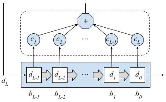
Figure 1. Linear feedback shift register.

Stream ciphers are mainly based on LFSRs defined over finite fields with $q=2$ [1]. Hence, the cell content is one bit, and the addition and multiplication correspond to XOR and AND operations, respectively. However, for efficiency reasons, in the generation process, LFSRs defined in $GF\left(2^n\right)$ are also being used in current communication systems. When LFSR is defined in this extension field, the cells contain n-bit words, where n matches the processor’s word length. Although the equations that govern the LFSR are the same, as described above, addition and multiplication are defined as polynomial addition and multiplication modulus $h\left(x\right)$, the polynomial used to construct the $GF\left(2^n\right)$. From now on, we shall use the notation $<L,p\left(x\right)>$ to refer to an LFSR with L cells in $GF\left(2\right)$ and connection polynomial $p\left(x\right)\in GF[2,x]$ of degree L. The form $<L,p\left(x\right),n>$ is for an LFSR of L cells in $GF\left(2^n\right)$ and connection polynomial $p\left(x\right)\in GF[2^n,x]$ of degree L.

2.2. Binary Equivalent Model

Komo and Lam [16] proposed a method to generate primitive polynomials in $GF\left(q^n\right)$ using primitive polynomials in $GF\left(q\right)$ based on the relationship previously discovered by Park and Komo [17] between the m-sequences produced in $GF\left(q^n\right)$ and $GF\left(q\right)$, in such a way that an m-sequence in $GF\left(q^m\right)$ can be decomposed into n m-sequences in $GF\left(q\right)$. More precisely:

Theorem 1

(cf. [17], th 7). Let $p\left(x\right)$ be a primitive polynomial of degree $m·n$ in $GF[q,x]$. Let $f\left(x\right)$ be one of the n primitive polynomials of degree m in $GF[q^n,x]$ into which $p\left(x\right)$ factors when viewed in $GF[q^n,x]$. Let $D=d_0,d_1,\cdots$ be an m-sequence over $GF\left(q^n\right)$ generated by $f\left(x\right)$. If

$$d_i=d_{i,0}{\lambda }_0+d_{i,1}{\lambda }_1+\cdots +d_{i,n-1}{\lambda }_n-1$$

(6)

where $\{{\lambda }_0,{\lambda }_1,\cdots ,{\lambda }_{n-1}\}$ is a basis for $GF\left(q^n\right)$ over $GF\left(q\right)$, then the sequence $d_{0,j},d_{1,j},\cdots$ is an m-sequence of length $q^{nm}-1$ over $GF\left(q\right)$.

As one can observe, the sequence $d_{0,j},d_{1,j},\cdots$ is composed by the j-th component of each element $d_i$ in the sequence D. Equivalently, the sequence $d_{0,j},d_{1,j},\cdots$ can be considered as a decimation sequence obtained from D giving rise to the following set of decimated sequences, as it is shown in Figure 2:

$$D^j=d_{0,j},d_{1,j},d_{2,j},\cdots ,$$

(7)

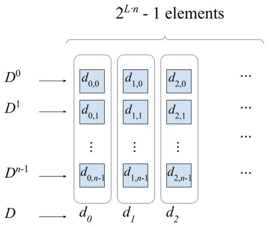
Figure 2. Relationship between m-sequences in the extended and base fields.

Furthermore, as it is stated in [16], since the sequences $D^j$, for $0\le j\le n-1$, are generated by the same polynomial $f\left(x\right)$, all of them are shifted versions of the same m-sequence. Hence, taking $D^0$ as the reference, we can define ${\theta }_j$ as the shift of $D^j$ respect to $D^0$. In [16], a method to obtain a primitive polynomial $f\left(x\right)\in GF[q^n,x]$ in terms of a given primitive polynomial $p\left(x\right)\in GF[q,x]$ is proposed by means of the computation of the shifts ${\theta }_j$ that satisfy the relationship between the m-sequences in the extended and base fields.

3. Efficient LFSR Implementation

The relationship between the m-sequences on $GF\left(2^n\right)$ and the m-sequences on $GF\left(2\right)$, as described in the previous section, also allows us to establish an equivalence between the LFSRs that generate them. This section presents a practical and efficient method to obtain such LFSRs, i.e., to obtain the feedback polynomial $p\left(x\right)$ and the seeds of each LFSR $<Ln,p\left(x\right)>$ that allow us to generate the same sequence as the LFSR $<L,f\left(x\right),n>$ from a given seed. Note that, according to the equivalent model, the n LFSRs in $GF\left(2\right)$ have the same connection polynomial $p\left(x\right)$ but different seeds, all of them related to the seed in $GF\left(2^n\right)$. Hence, in order to efficiently implement the LFSR $<L,f\left(x\right),n>$ using the equivalent model, it is necessary to solve three main questions: the computation of $p\left(x\right)$, the computation of the seeds, and how to speed up the performance of the binary LFSRs.

Since the connection polynomial $f\left(x\right)$ is primitive, the minimal polynomial $p\left(x\right)$ of the decimated sequences $D^i$ is also primitive and unique for $0\le i\le n-1$. Hence, $p\left(x\right)$ can be obtained analyzing a decimated sequence using the Massey–Berlekamp algorithm [18]. Consequently, the following Algorithm 1 is defined.

Algorithm 1: Computation of connection polynomial $p\left(x\right)$.

input  : LFSR $<L,f\left(x\right),n>$  output: $p\left(x\right)$ in LFSR $<Ln,p\left(x\right)>$ Implement the LFSR$<L,f\left(x\right),n>$; Generate$2Ln+1$elements, at least, using any nonzero seed; Obtain a decimated sequence$D^i$for any$i,0\le i\le n-1$; Obtain the minimal polynomial$p\left(x\right)$of the$D^i$generated in step 3

Once $p\left(x\right)$ has been determined, we can construct the n LFSRs $<Ln,p\left(x\right)>$, but we need their respective seeds in order to generate the same sequence as that generated from the initial seed $s=(d_0,d_1,\cdots ,d_{L-1})$ in the extended field. As it is derived from the equivalent model, the L known elements in $GF\left(2^n\right)$ that compose the initial seed only provide us with $nL$ bits, while $n^{2}L$ bits are needed to complete the n seeds in $GF\left(2\right)$ (see Figure 3). Thus, the seed $s^j$ of $D^j$ can be partially written in terms of the seed s of D as:

$$s^j=d_{0,j},d_{1,j},\cdots ,d_{L-1,j},d_{L,j},\cdots ,d_{n·L-1,j}$$

(8)

where $d_{L,j},\cdots ,d_{n·L-1,j}$ are unknown for $0\le j\le n-1$. However, the shifts ${\theta }_i$ that relate the binary sequences to each other allow us to obtain the seeds completely. The following subsections describes the computation of ${\theta }_j$ and $s^j$.

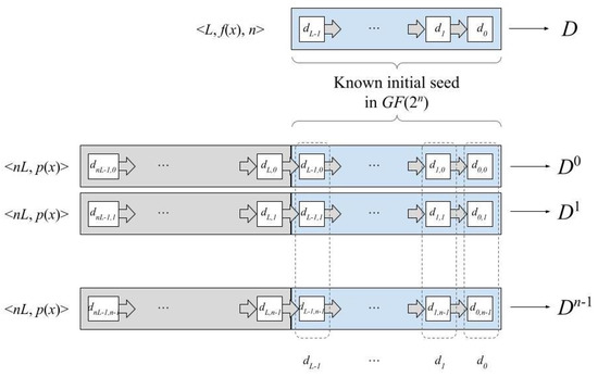
Figure 3. LFSR seeds in the binary equivalent model.

3.1. Computation of Shifts

All decimated sequences $D^j$ have the same primitive minimal polynomial $p\left(x\right)$, obtained using Algorithm 1. Hence, all of them are shifted versions of the others. The shift ${\theta }_j$ of $D^j$ with respect to $D^0$ allows one to obtain the state of the j-th LFSR (the one that generates $D^j$) from the state of the 0-th LFSR as follows:

$$(d_{0,j},d_{1,j},\cdots ,d_{n·L-1,j})=(d_{0,0},d_{1,0},\cdots ,d_{n·L-1,0})A^{{\theta }_j},$$

(9)

where A is the connection matrix of $p\left(x\right)$, that is:

$$A=\left[\begin{array}{ccccc}0& 0& \cdots & 0& c_{n·L}\\ 1& 0& \cdots & 0& c_{n·L-1}\\ 0& 1& \cdots & 0& c_{n·L-2}\\ ⋮& ⋮& \ddots & ⋮& ⋮\\ 0& 0& \cdots & 1& c_1\end{array}\right]$$

(10)

The computation of ${\theta }_j$ is not an easy task. Furthermore, the computation of $A^{{\theta }_j}$ is time-consuming. Instead, we can obtain the matrix $A^{\left(j\right)}=A^{{\theta }_j}$ solving the linear equation system of Equation (9). Note that we have n matrices $A^{\left(j\right)}$ to compute and thus n linear systems to solve. The linear system in Equation (9), stated using the first $nL$ element, the seed, has $nL$ equations and $n^2{L}^2$ unknowns. Each new element of the sequence defines $nL$ new equations with the same unknowns. Hence, the $2Ln+1$ elements of the m-sequence in $GF\left(2^n\right)$ generated in Algorithm 1 to obtain $p\left(x\right)$ provide enough equations to solve the systems. As an example, we consider a 3-stage LFSR defined in $GF\left(2^4\right)$, that is, the LFSR $<3,f\left(x\right),4>$, where $f\left(x\right)=1+x+\left(0x9\right)x^3$ is primitive over $GF\left(2^4\right)$ and the primitive polynomial $x^4+x+1$ has been used to construct $GF\left(2^4\right)$. From the initial seed $(1,1,1,1),(0,0,0,0),(0,1,1,0)$ or, equivalently, $(1+\alpha +{\alpha }^2+{\alpha }^3,0,\alpha +{\alpha }^2)$, $\alpha$ being a root of $x^4+x+1$, the LFSR $<3,f\left(x\right),4>$ generates the following sequence:

$$\begin{array}{c}001000001100111010010000\cdots \\ 101001011000000001010001\cdots \\ 101110100000001111001000\cdots \\ 001110000001000101100011\cdots \end{array}$$

(11)

where the elements of $GF\left(2^4\right)$ are represented in columns with the least significant bit at the top. The four decimated sequences are all generated by the same primitive polynomial $p\left(x\right)=x^{12}+x^6+x^5+x^3+1$ and, hence, all of them are shifted versions of the same m-sequence. Solving the system in Equation (9), we obtain the matrices $A^{\left(1\right)},A^{\left(2\right)},A^{\left(3\right)}$:

$$A^{\left(1\right)}=\left[\begin{array}{c}100000000110\\ 010000000011\\ 101000000001\\ 110100000000\\ 011010000000\\ 001101000000\\ 000110100110\\ 000011010101\\ 000001101010\\ 000000110011\\ 000000011001\\ 000000001100\end{array}\right]A^{\left(2\right)}=\left[\begin{array}{c}000000101010\\ 000000010101\\ 100000001010\\ 110000000101\\ 111000000010\\ 011100000001\\ 101110101010\\ 010111111111\\ 001011111111\\ 000101010101\\ 000010101010\\ 000001010101\end{array}\right]A^{\left(3\right)}=\left[\begin{array}{c}000111111111\\ 000011111111\\ 000001111111\\ 000000111111\\ 100000011111\\ 010000001111\\ 001111111000\\ 100000000011\\ 110000000001\\ 111111111111\\ 011111111111\\ 001111111111\end{array}\right]$$

(12)

Since the decimated sequences have a small period of $2^{12}-1=4095$, we have also compared them to obtain the shifts ${\theta }_1=3276$, ${\theta }_2=3549$, and ${\theta }_3=3822$. In a real scenario, ${\theta }_j$ is not going to be computed. It is important to point out that the calculation of the $A^{\left(j\right)}$ matrices can be performed prior to the normal operation of the LFSR since they do not depend on the seeds.

3.2. Computation of Seeds

Let us consider that the shift matrices $A^{\left(j\right)}=A^{{\theta }_j}$ have already been precomputed. For any given seed $(d_0,d_1,\cdots ,d_{L-1})$, the seeds of the binary LFSRs can be represented as:

$$(d_{0,j},d_{1,j},\cdots ,d_{n·L-1,j})=(d_{0,0},d_{1,0},\cdots ,d_{n·L-1,0})A^{\left(j\right)},$$

(13)

where $d_{L,j},\cdots ,d_{n·L-1,j}$ are unknowns for every $0\le j\le n-1$. The values $d_{L,0},$$\cdots ,$$d_{n·L-1,0}$ can be obtained solving the linear system composed with the $(n·L-L)$ equations with the known values $d_{0,j},d_{1,j},\cdots ,d_{L-1,j},$ for $0\le j\le n-1$, i.e.:

$$d_{i,j}=\sum _{k=0}^{n·L-1}{d}_{k,0}{a}_{k,i}^{\left(j\right)},0\le i\le L-1,1\le j\le n-1,$$

(14)

where $a_{k,i}^{\left(j\right)}$ are the components of the matrix $A^{\left(j\right)}$. The remaining seeds $(d_{0,j},d_{1,j},$$\cdots ,d_{n·L-1,j})$, with $1\le j\le L-1$, are calculated using Equation (13). Considering the precomputed matrices in Equation (12) of the previous example, the Equation (13) can be written as:

$$\begin{array}{c}(1,0,1,d_{3,1},\cdots ,d_{11,1})=(0,0,1,d_{3,0},\cdots ,d_{11,0})A^{\left(1\right)}\\ (1,0,1,d_{3,2},\cdots ,d_{11,2})=(0,0,1,d_{3,0},\cdots ,d_{11,0})A^{\left(2\right)}\\ (0,0,1,d_{3,3},\cdots ,d_{11,3})=(0,0,1,d_{3,0},\cdots ,d_{11,0})A^{\left(3\right)}\end{array}$$

(15)

Solving for $(d_{3,0},\cdots ,d_{11,0})$, we obtained the complete seed for the sequence $D^0$, that is, $(0,0,1,0,0,0,0,0,1,1,0)$. Next, using the matrices $A^{\left(1\right)}$, $A^{\left(2\right)}$ and $A^{\left(3\right)}$, the complete seeds of the sequences $D^1$, $D^2$, and $D^3$ are obtained. Hence, we have:

$$\begin{array}{c}see{d}_0=(0,0,1,0,0,0,0,0,1,1,0)\\ see{d}_1=(1,0,1,0,0,1,0,1,1,0,0)\\ see{d}_2=(1,0,1,1,1,0,1,0,0,0,0)\\ see{d}_3=(0,0,1,1,1,0,0,0,0,0,0)\end{array}$$

(16)

3.3. Grouped Operations

Once the n binary LFSRs have been constructed, it is time to generate the sequence. Instead of running n independent instances of the binary LFSR, which require 1-bit operations with an n-bit processor, we propose to group the n LFSRs into a unique LFSR with connection polynomial $p\left(x\right)$ but using n-bit cells. The result is not an LFSR over $GF\left(2^n\right)$ but a parallel implementation of n LFSR over $GF\left(2\right)$ using only one processor. Since the addition and multiplication in the binary LFSRs correspond to the XOR and AND bitwise operations, respectively, instead of applying the XOR to 1-bit values, we apply it over n-bit values. The processor takes the same time to perform the XOR operation with 1-bit values than with n-bit values because the word length is n, thus saving a lot of execution time. Hence, Equation (4) can be redefined as follows:

$$\left[\begin{array}{c}{d}_{i,0}\\ ⋮\\ d_{i,n-1}\end{array}\right]=c_1\left[\begin{array}{c}{d}_{i-1,0}\\ ⋮\\ d_{i-1,n-1}\end{array}\right]+c_2\left[\begin{array}{c}{d}_{i-2,0}\\ ⋮\\ d_{i-2,n-1}\end{array}\right]+\cdots +c_L\left[\begin{array}{c}{d}_{i-Ln,0}\\ ⋮\\ d_{i-Ln,n-1}\end{array}\right],$$

(17)

in such a way that the n sequences stated in Equation (7) are simultaneously generated using a unique polynomial $p\left(x\right)$ (see Equation (5)).

From the practical implementation perspective, there is no difference at all with respect to preforming a classical binary LFSR, which includes coding and execution, since the 1-bit XOR operation is actually performed taking n-bit operands. Hence, the n-bit grouped operation proposed in this paper is a way of not wasting the capacity of the operations of the n-bit processors. As a consequence, this implementation method increases the bit generation net rate by n because the generation of a new element of a 32-bit m-sequence takes the same amount of time as a new element of a 1-bit m-sequence.

4. Primitiveness Test

As mentioned in Section 2.2, the m-sequences generated by an LFSR in $GF\left(2^n\right)$ can be decomposed into n m-sequences generated by n LFSRs in $GF\left(2\right)$, so that when the feedback polynomial of the LFSR in the extended field is primitive, all LFSRs in $GF\left(2\right)$ have the same feedback polynomial, and it is also primitive. This relationship is what allows us to propose an algorithm to check if a polynomial is primitive over $GF\left(2^n\right)$.

In general terms, to check if a polynomial $f\left(x\right)$ over $GF\left(2^n\right)$ is primitive, we propose to build an LFSR whose feedback polynomial is $f\left(x\right)$ and generate $2·m·n+1$ elements, at least. The sequence generated by concatenating all generated elements is decomposed into n binary sequences by decimating by n, as it is stated in Equation (7). Next, the n sequences are processed to obtain the minimal polynomials of the binary LFSRs that generate them (This can be achieved using the Berlekamp–Massey algorithm). If all the n sequences are generated by the same polynomial and it is also primitive, then $f\left(x\right)$ is primitive over $GF\left(2^n\right)$. Algorithm 1 can be extended including one more step (step 5) to perform the check, resulting in Algorithm 2.

Algorithm 2: Primitiveness test.

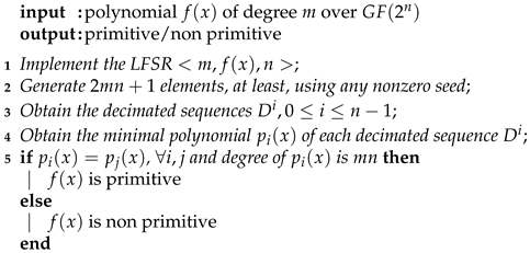As an example, let us consider the degree 6 polynomial $f\left(x\right)=0x1+0x2·x+0x4·x^2+0x8·x^3+0x5·x^4+0x9·x^5+x^6\in GF[2^4,x]$, where the primitive polynomial $h\left(x\right)=x^4+x+1$ has been used to construct $GF\left(2^4\right)$. In order to check if $f\left(x\right)$ is primitive, we consider $f\left(x\right)$ as the feedback polynomial of an LFSR in the $GF\left(2^4\right)$ of 6 cells. For a random seed $(0x9,0x4,0x5,0x9,0x5,0x1)$, we generate $2mn+1=49$ elements, giving rise to the following decimated sequences:

$$\begin{array}{c}{D}^0=0010011011100000011010110001000000101011001111100\\ D^1=0101100111010011110000001010111101111001011010001\\ D^2=0000000011000101110101100100010010011000001000101\\ D^3=1111011111000011001111010101101110100100010100001\end{array}$$

(18)

The same minimal polynomial $p\left(x\right)$ is obtained for each $D^i$ sequence by means of the Massey–Berlekamp algorithm [18]. The polynomial is the following:

$$p\left(x\right)=x^{24}+x^{23}+x^{22}+x^{21}+x^{20}+x^{19}+x^{15}+x^{14}+x^9+x^8+x^7+x^6+1$$

(19)

Since $p\left(x\right)$ is primitive over $GF\left(2\right)$, we can conclude that $f\left(x\right)$ is primitive over $GF\left(2^4\right)$.

5. Efficiency and Security

The implementation presented in Section 3 considerably reduces the execution time of the LFSRs defined in $GF\left(2^n\right)$. Specifically, an implementation of the LFSR used in the SNOW 3G stream cipher has been performed and compared with the implementation provided in the technical specification of the protocol [10]. This is an LFSR $<16,f\left(x\right),32>$. Hence, the equivalent model is based on 32 LFSRs $<512,p\left(x\right)>$. The polynomial $p\left(x\right)$ is built from 1024 elements generated using the official implementation [10] following the steps established in Algorithm 1. The result is that the 32 decimated sequences have the same minimal polynomial $p\left(x\right)$ of degree 512, whose coefficients are represented below in compact hexadecimal format:

$$\begin{array}{c}\hfill 84009C624D4F75F17EDA41C663C5DFDED8A535DA1C5F70824152A7\end{array}$$

(20)

$$\begin{array}{c}\hfill C23EDB90D572852A765FF5F2012A64F5D3FD361B005ADBA45A1995\end{array}$$

(21)

$$\begin{array}{c}\hfill \hspace{1em}\hspace{1em}\hspace{1em}\hspace{1em}\hspace{1em}\hspace{1em}\hspace{1em}\hspace{1em}\hspace{1em}\hspace{1em}\hspace{1em}\hspace{1em}\hspace{1em}\hspace{1em}\hspace{1em}\hspace{1em}\hspace{1em}\hspace{1em}E64E48362706D62606828\end{array}$$

(22)

Despite the fact that $p\left(x\right)$ has 250 non-zero coefficients, and therefore 250 XOR operations are required to generate the next element in the sequence, the execution time is 3.3 times lower than the original implementation. The computation of the matrices $A^{\left(j\right)}$ is not considered, since this is performed prior to the normal operating of the LFSR. The times have been calculated by taking the average of 10 repetitions of each generation of 1000, 10,000, 20,000, 50,000, and 100,000 elements. Both implementations have been made in Python 3.9 language and have been executed on an Intel(R) Core(TM) i7-10510U 64-bit processor with 16 GB of RAM. Although the SNOW 3G algorithm has been designed to be executed on 32-bit platforms, the tests carried out on a 64-bit processor are completely valid since the greater word length of the processor compared to the algorithm does not affect the normal execution of our implementation. Note that the goal is to achieve an implementation of an algorithm defined in $GF\left(2^n\right)$ using n-bit operations. The case of working with processors of more than n bits offers the possibility of developing new faster implementations to make the most of their capacity, but requires adapting the algorithms to the new processor architecture. This is outside the scope of this work.

As mentioned in the Section 3, the net bit generation rate is increased by n when compared to a single binary LFSR implementation, that is, to a binary LFSR using the same connection polynomial. However, the improvement observed in the tests on SNOW 3G does not reach the net rate. This is mainly due to the number of non-zero coefficients in $p\left(x\right)$ that slow down the computation. Therefore, in the case of equivalent binary polynomials $p\left(x\right)$ with a few nonzero coefficients, the real rate will reach the net rate. In the general case, the fewer non-zero coefficients in $p\left(x\right)$, the greater the improvement to the generation rate.

The efficiency of the proposed implementations, shown in Section 3 affects the security of the cryptosystems used by these LFSRs, although, in general, they are not intended to replace those currently used by most devices, such as smartphones, but rather for use in mobile devices without any type of restriction, such as personal computers or servers. Using the equivalent model implies multiplying by n, the number of bits needed to generate a new element of the m-sequence over $GF\left(2^n\right)$, that is, to generate n bits. In the case of SNOW 3G, it goes from 512 to 16,384 bits. Therefore, the theoretical improvement of the execution time by a factor n is associated with an increase in the same factor n in the amount of memory needed to generate the same number of bits. As a consequence, this implementation provides a substantial improvement for the calculation of m-sequences that, although it could not be deployed on some devices, could always be used for cryptanalysis tasks. Regarding the cost of our proposal, an increment in the memory cells must be taken in mind, rising from $nL$ to $n^{2}L$ bits.

Regarding the algorithm for primitiveness testing, we can conclude that it has a better performance than O’Connor’s algorithm, one of the most used ones. The main advantage is that the proposed algorithm has to generate $2mn+1$ elements instead of the whole sequence or alternatively to perform as many divisions as elements in the maximal sequence over the extended field. The validation and comparison tests have been performed using Mathematica software, version $\mathrm{10.0.0}$, on a 64-bits Microsoft Windows platform running on a Intel(R) Core (TM) processor with i7-4510U CPU @ $2.00$ GHz and 16 GB RAM. The processor’s temperature and the amount of simultaneous running processes have been taken into account for the execution time comparison. Figure 4 shows the behavior of the algorithm with respect to O’Connor’s in $GF\left(2^8\right)$ and $GF\left(2^{16}\right)$, respectively.

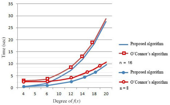
Figure 4. Execution time in $GF\left(2^8\right)$ and $GF\left(2^{16}\right)$.

6. Conclusions

In this article, we have presented two real applications of the relationships between the m-sequences in $GF\left(2^n\right)$ and $GF\left(2\right)$. The first one is a new algorithm designed to verify the primitiveness of polynomials with coefficients in $GF\left(2^n\right)$ that improves the execution times of existing methods. The second one is the support of an efficient implementation of the LFSRs defined over the extended field $GF\left(2^n\right)$, which improves the other implementations. It enables better performance of the LFSR-based stream ciphers, often used in high speed communication systems. The improvement is achieved by a combination of the binary equivalent model of LFSRs in the extended field, which uses only binary operations, and the n-bit grouped operation that take advantage of the n-bit processors. The feasibility of the implementation has been shown by applying it to the SNOW 3G stream cipher, whose execution time has been reduced by a factor of 3.3 with respect to the code provided in the technical specification of the protocol. These results can also be extended to cryptanalysis, making use of not only the grouped operations but of the underlying binary structure that may facilitate the parallelization of the operations. On the other hand, the proposed implementation is software-oriented, although the binary operations also allow hardware implementations. In this way, we provide a complete method to efficiently increase the bit generation rate.

References

- Menezes, A.J.; Van Oorschot, P.C.; Vanstone, S.A. Handbook of Applied Cryptography; CRC Press: Boca Ratón, FL, USA, 2020. [Google Scholar]
- Shannon, C. Communication Theory of Secrecy Systems. Bell Syst. Tech. J. 1949, 28, 656–715. [Google Scholar] [CrossRef]
- Golomb, S.W. Shift Register Sequences, 3rd Revised ed.; Aegean Park Press: Laguna Hills, CA, USA, 2017. [Google Scholar]
- Padgette, J.; Bahr, J.; Batra, M.; Holtmann, M.; Smithbey, R.; Lily, C.; Scarfone, K. Guide to Bluetooth Security; NIST: Gaithersburg, MD, USA, 2017. [Google Scholar]
- Jindal, P.; Singh, B. RC4 Encryption-A Literature Survey. Procedia Comput. Sci. 2015, 46, 697–705. [Google Scholar] [CrossRef] [Green Version]
- Biham, E.; Dunkelman, O. Cryptanalysis of the A5/1 GSM stream cipher. In Proceedings of the International Conference on Cryptology in India, Calcutta, India, 10–13 December 2000; pp. 43–51. [Google Scholar]
- Kiyomoto, S.; Tanaka, T.; Sakurai, K. K2: A stream cipher algorithm using dynamic feedback control. In Proceedings of the International Conference on Security and Cryptography, SECRYPT, Barcelona, Spain, 28–13 July 2007; Hernando, J., Fernández-Medina, E., Malek, M., Eds.; INSTICC Press: Lisboa, Portugal, 2007; pp. 204–213. [Google Scholar]
- George, K.; Michaels, A.J. Designing a Block Cipher in Galois Extension Fields for IoT Security. IoT 2021, 2, 669–687. [Google Scholar] [CrossRef]
- Panario, D.; Reis, L. The functional graph of linear maps over finite fields and applications. Des. Codes Cryptogr. 2019, 87, 437–453. [Google Scholar] [CrossRef]
- ETSI/SAGE. Specification of the 3GPP, Confidentiality and Integrity Algorithm UEA2 and UIA2; Document 2: SNOW 3G Specification; ETSI: Sophia Antipolis, France, 2006. [Google Scholar]
- Caforio, A.; Balli, F.; Banik, S. Melting SNOW-V: Improved lightweight architectures. J. Cryptogr. Eng. 2020, 12, 53–73. [Google Scholar] [CrossRef]
- Ekdahl, P.; Johansson, T.; Maximov, A.; Yang, J. A new SNOW stream cipher called SNOW-V. IACR Trans. Symmetr. Cryptol. 2019, 3, 1–42. [Google Scholar] [CrossRef]
- Ekdahl, P.; Maximov, A. SNOW-Vi: An Extreme Performance Variant of SNOW-V for Lower Grade CPUs. In Proceedings of the 14th ACM Conference on Security and Privacy in Wireless and Mobile Networks, WiSec ’21, Abu Dhabi, United Arab Emirates, 28 June–2 July 2021; pp. 261–272. [Google Scholar]
- Avanzi, R.; Theriault, N. Effects of optimization for software implementations of small binary field arithmetic. In International Workshop on the Arithmetic of Finite Fields; Springer: Berlin/Heidelberg, Germany, 2007; pp. 69–84. [Google Scholar]
- Delgado-Mohatar, O.; Fúster-Sabater, A.; Sierra, J.M. Performance evaluation of highly efficient techniques for software implementation of LFSR. Comput. Electr. Eng. 2011, 37, 1222–1231. [Google Scholar] [CrossRef]
- Komo, J.J.; Lam, M.S. Primitive Polynomials and m-sequences over GF(qm). IEEE Trans. Inf. Theory 1993, 39, 643–647. [Google Scholar] [CrossRef]
- Park, W.J.; Komo, J.J. Relationships Between m-Sequences over GF(q) and GF(qm). IEEE Trans. Inf. Theory 1989, 35, 183–186. [Google Scholar] [CrossRef]
- Massey, J.L. Shift register synthesis and BCH decoding. IEEE Trans. Inf. Theory 1969, 15, 122–127. [Google Scholar] [CrossRef] [Green Version]
Publisher’s Note: MDPI stays neutral with regard to jurisdictional claims in published maps and institutional affiliations. |
© 2022 by the authors. Licensee MDPI, Basel, Switzerland. This article is an open access article distributed under the terms and conditions of the Creative Commons Attribution (CC BY) license (https://creativecommons.org/licenses/by/4.0/).