A Formal Analysis of Generalized Peterson’s Syllogisms Related to Graded Peterson’s Cube

Abstract

This publication builds on previous publications in which we constructed syntactic proofs of fuzzy Peterson’s syllogisms related to the graded square of opposition. The aim of the publication is to be formally able to find syntactic proofs of fuzzy Peterson’s logical syllogisms with forms of fuzzy intermediate quantifiers that design the graded Peterson’s cube of opposition.

1. Introduction

The article aims to follow up on the achieved results concerning the formal proofs of fuzzy Peterson syllogisms.

The theory of syllogistic reasoning was investigated by several authors as a generalization of classical Aristotelian syllogisms ([1,2,3]). Categorical syllogisms ([4,5]) consist of three main parts: the major premise, the minor premise, and the conclusion. With the introduction of the term “generalized quantifier“, which was proposed by Mostowski in [6], the study of logical syllogisms expanded to a group of generalized logical syllogisms. Such syllogisms include forms that contain different types of generalized quantifiers. One special group is intermediate quantifiers. This topic started to be interesting for linguists and philosophers, who laid a question of how to explain expressions that represent generalized quantifiers.

Peterson, in his book [7], is interested in the group of intermediate quantifiers which lie between classical quantifiers. He first philosophically analyzed and explained the meaning of intermediate quantifiers in terms of their position in the generalized square of opposition. Furthermore, he continued the study of the group of generalized logical syllogisms. Peterson’s enlargement was established on an idea to substitute a classical quantifier with an intermediate one in the classical four figures, which returned in 105 new valid intermediate syllogisms. A check of the validity of a group of logical syllogisms was conducted using Venn diagrams, which was carried out by several authors [7,8,9]. Below, we present an example of a non-trivial fuzzy intermediate syllogism as follows:

$P_1:$ Almost all people do not have a plane.

$P_2:$ Most people have a phone.

$C:$ Some people who have a phone do not have a plane.

The work of authors who dealt with generalized quantifiers was followed by several authors with the advent of the definition of a fuzzy set. Several authors followed up this approach. They introduced several forms of logical syllogisms with fuzzy generalized quantifiers. In 1985, L. Zadeh semantically interpreted a special group of fuzzy syllogisms with fuzzy intermediate quantifiers in both premises as well as in the conclusion. Below, we present a very famous multiplicative chaining syllogism ([10]) as follows:

$Q_1$Y is M

$Q_2$M is X

$(\ge Q_1\otimes Q_2)$Y are X.

As was explained by Zadeh, the expression $\ge Q_1\otimes Q_2$ in the conclusion of Zadeh’s syllogism can be read as “at least $Q_1\otimes Q_2$”.

Zadeh’s work was later extended and sophisticated by many authors. From the point of view of fuzzy quantifiers, which are represented as intervals in Didier Duboise’s approach in ([11,12]), Zadeh’s special syllogism is compared by M. Pereira-Fariña in [13]. In the publications, Dubois et al. work with quantifiers represented as crisp closed intervals (more than a half $=[0.5,1]$, around five $=[4,6]$). A typical example of such interval fuzzy syllogism appears as follows:

$P_1$: $[5\%,10\%]$ students have a job.

$P_2$: $[5\%,10\%]$ students have a child.

C: $[0\%,10\%]$ students have a child and have a job.

Recall that a global overview of fuzzy generalized quantifiers and the various mechanisms for defining these quantifiers can be found in [14].

M. Pereira-Fariña et al. follow, in the next publication [15], by interpreting logical syllogisms with more premises. In this publication, a group of authors suggested a general inference schema for syllogistic reasoning, which was proposed as the transformation of the syllogistic reasoning study into an equivalent optimization problem.

The above-mentioned publications study and verify the validity of fuzzy syllogisms, especially semantically. In [16], a mathematical definition of fuzzy intermediate quantifiers based on the theory of evaluative linguistic expressions was proposed. The motivation, fundamental assumptions, and formalization of this theory are described in detail in [17]. Later, in [18], we focused on the syntactic construction of proofs of all 105 basic fuzzy logical syllogisms that relate to the graded Peterson’s square of opposition (see [19]). Typical examples of natural language expressions contained in Peterson’s logical syllogisms are as follows:

Most children like computer games.

Most cats like to sleep.

1.1. Application of Generalized Quantifiers

Generalized quantifiers offer several types of applications in economics, medicine, heavy industry, biology, etc. Let us first mention applications related to a group of fuzzy intermediate quantifiers which are represented by natural language expressions. One of the interesting applications is time series prediction, which has its application mainly in economic fields. In [20], the author proposed an interpretation, forecasting, and linguistic characterization of time series. The result makes it possible to obtain information about the data using natural language, which is much more understandable to the average user. To illustrate the reader, we present an example of the linguistic interpretation of economic time series, using natural language, as follows:

Most (many, few) analyzed time series stagnated recently, but their future trend is slightly increasing [20].

Another area that is very closely related to this application is getting new information from natural language data. Here, it is offered to use the theory of syllogistic reasoning and to obtain new information from natural language data using valid forms of syllogisms. Time series were also analyzed by a group of authors in [21]. There are also publications of authors who are interested in the linguistic summarization of data. In [22], the authors introduced methods for using the linguistic database to summarize natural data (see [23,24,25,26]). Later, these methods were improved in [27] and implemented by Kasprzyk and Zadrożny [28]. Another linguistic summarization of process data was proposed in [29].

Another area of application is the use of fuzzy association analysis and the use of association rules to interpret natural language data. An algorithm for the interpretation of biological data using fuzzy intermediate quantifiers was proposed in [30].

Most irises with both small-length sepals and petals have small-width petals.

1.2. Main Goals

The main idea of this publication is to work with terms that also contain negated terms in the antecedent, and to study related valid fuzzy syllogisms. Typical examples of natural language expressions which are related to the graded Peterson’s ([19]) cube are as follows:

Almost all students who do not like mathematics do not study technical fields.

Most people who do not drink alcohol have healthy livers.

A typical example of a syllogism with fuzzy intermediate quantifiers in both premises, which is called non-trivial, reads as follows:

$P_1:$ Almost all people who do sports have healthy lungs.

$P_2:$ Almost all people who do sports do not have asthma.

$C:$ Some people who do not have asthma have healthy lungs.

1.3. Application of New Forms of Fuzzy Intermediate Quantifiers

As mentioned above, there are several application areas where natural language expressions are used. We also gave, in the previous section, specific examples of natural language expressions that occur in both of the premises of syllogisms or are used to interpret natural data. Therefore, the idea is offered to first find and formally prove the validity of new forms of logical syllogisms, and further, to work on the use of these forms in the areas of fuzzy association analysis, language interpretation, linguistic summarization, the interpretation of time series, etc.

The paper is structured as follows: after the motivational introduction, the reader is acquainted with mathematical theory in the methods section. The third section contains important mathematical definitions of new forms of intermediate quantifiers. In this section, we follow with proofs of new forms of logical syllogisms. The results section is closed by concrete examples of valid forms of logical syllogisms. This section continues with a discussion section, in which we summarize the results achieved. We conclude this paper with a conclusion and statement of future directions.

2. Main Methods

The main approach of this section is to recall the theory of fuzzy natural logic (FNL) that was designed based on the fuzzy type theory (FTT). FNL is a formal mathematical theory that includes three theories:

• Theory of evaluative linguistic expressions (see [17]);
• Theory of fuzzy IF–THEN rules and approximate reasoning (see [31]);
• Theory of intermediate quantifiers, generalized syllogisms, and graded structures of opposition (see [16,18]).

2.1. Fuzzy Type Theory

This section focuses on the reminder of the main symbols and of the fuzzy type theory. We will not repeat all the details here; we refer readers to previous publications [17,32].

Let us recall, at this point, that the mathematical theory of fuzzy quantifiers was proposed over the Łukasiewicz fuzzy type theory (Ł-FTT). The structure of truth values is represented by a linearly ordered MV${}_{\mathbf{\Delta }}$-algebra that is extended by the delta operation (see [33,34]). A particular case is the standard Łukasiewicz MV${}_{\Delta }$-algebra:

$$\mathcal{L}=\langle [0,1],\mathbf{\vee },\mathbf{\wedge },\otimes ,\to ,0,1,\Delta \rangle .$$

(1)

The fundamental objects that represent the syntax of Ł-FTT are classical (cf. [35]). We assume atomic types as follows: $ϵ$ (elements) and o (truth values). General types are marked by Greek letters $\alpha ,\beta ,\dots$. A set of all types is marked by Types. The (meta-)symbol “$:=$” used below means “is defined by”.

The language contains of variables $x_{\alpha },\dots$, special constants $c_{\alpha },\dots$ ($\alpha \in$ Types), symbol $\lambda$, and parentheses. The connectives are fuzzy equality/equivalence ≡, conjunction ∧, implication ⇒, negation ¬, strong conjunction &, strong disjunction ∇, disjunction ∨, and delta $\mathbf{\Delta }$. The fuzzy type theory is complete, i.e., a theory T is consistent iff it has a (Henkin) model ($\mathcal{M}\vDash T$). We sometimes use the equivalent notion: $T⊢A_o$ iff $T\vDash A_o$.

The following special formulas are important in our theory below:

$$\begin{array}{ccc}\hfill {\mathrm{{\rm Y}}}_{oo}& \equiv \lambda z_o·\mathbf{\neg }\mathbf{\Delta }(\mathbf{\neg }{z}_o),\hfill & \hfill (\mathrm{nonzero} \mathrm{truth} \mathrm{value})\\ \hfill {\widehat{\mathrm{{\rm Y}}}}_{oo}& \equiv \lambda z_o·\mathbf{\neg }\mathbf{\Delta }(z_o\mathbf{\vee }\mathbf{\neg }{z}_o).\hfill & \hfill (\mathrm{general} \mathrm{truth} \mathrm{value})\end{array}$$

Thus, $\mathcal{M}\left(\mathrm{{\rm Y}}\left(A_o\right)\right)=1$ iff $\mathcal{M}\left(A_o\right)>0$, and $\mathcal{M}\left(\widehat{\mathrm{{\rm Y}}}\left(A_o\right)\right)=1$ iff $\mathcal{M}\left(A_o\right)\in (0,1)$ holds in any model $\mathcal{M}$.

2.2. Evaluative Linguistic Expressions

As we stated in the introduction, the formal definitions of fuzzy intermediate quantifiers are based on evaluation linguistic expressions. In this subsection, we recall the theory of evaluative linguistic expressions.

Evaluative linguistic expressions are special expressions of a natural language, for example, very small, roughly medium, extremely large, very long, quite roughly, extremely rich, etc. Their theory is the main part of the fuzzy natural logic. The evaluative language expressions themselves play an important role in everyday human reasoning. We can find them in a wide variety of areas, such as economics, decision making, and more.

The language $J^{\mathrm{Ev}}$ contains special symbols as follows:

• The constants $\top ,\perp \in {Form}_o$ for truth and falsity, and $†\in {Form}_o$ for the middle truth value;
• A special constant $\sim \in {Form}_{\left(oo\right)o}$ for an additional fuzzy equality on the set of truth values L;
• A set of special constants $\mathbf{\nu },\dots \in {Form}_{oo}$ for linguistic hedges. The $J^{\mathrm{Ev}}$ contains the following special constants: $\{Ex,Si,Ve$, $ML,Ro,QR,VR\}$’ these denote the linguistic hedges: (extremely, significantly, very, roughly, more or less, rather, quite roughly, and very roughly, respectively);
• A set of triples of next constants $({\mathbf{a}}_{\mathbf{\nu }},{\mathbf{b}}_{\mathbf{\nu }},{\mathbf{c}}_{\mathbf{\nu }}),\dots \in {Form}_o$, where each hedge $\mathbf{\nu }$ is uniquely connected with one triple of these constants.

The evaluative expressions are interpreted by special formulas $\mathit{Sm}\in {Form}_{oo\left(oo\right)}$ (small), $\mathit{Me}\in {Form}_{oo\left(oo\right)}$ (medium), $\mathit{Bi}\in {Form}_{oo\left(oo\right)}$ (big), and $\mathit{Ze}\in {Form}_{oo\left(oo\right)}$ (zero) that can be expanded by several linguistic hedges. Let us remind that a hedge, which is often an adverb such as “extremely, significantly, very, roughly”, etc., is, in general, represented by a formula $\mathbf{\nu }\in {Form}_{oo}$ with specific properties. We proposed a formula $Hedge\in {Form}_{o\left(oo\right)}$. Then, $T^{\mathrm{Ev}}⊢Hedge\mathbf{\nu }$ means that $\mathbf{\nu }$ is a hedge. The other details can be found in [17]. The formula $T^{\mathrm{Ev}}⊢Hedge\mathbf{\nu }$ is provable for all $\mathbf{\nu }\in \{Ex,Si,Ve$, $ML,Ro,QR,VR\}$. Furthermore, evaluative linguistic expressions are represented by formulas:

$$\mathit{Sm}\mathbf{\nu },\mathit{Me}\mathbf{\nu },\mathit{Bi}\mathbf{\nu },\mathit{Ze}\mathbf{\nu }\in {Form}_{oo},$$

(2)

where $\mathbf{\nu }$ is a hedge. We will also assume an empty hedge $\overline{\mathbf{\nu }}$ that is introduced in front of small, medium, and big if no other hedge is assumed. A special hedge is ${\mathbf{\Delta }}_{oo}$, that represents the expression “utmost” and occurs below in the evaluative expression $\mathit{Bi}\mathbf{\Delta }$.

Let ${\mathbf{\nu }}_{1,oo},{\mathbf{\nu }}_{2,oo}$ be two hedges, i.e., $T^{\mathit{Ev}}⊢Hedge{\mathbf{\nu }}_{1,oo}\mathrm{and}{T}^{\mathit{Ev}}⊢Hedge{\mathbf{\nu }}_{2,oo}$. We propose a relation of the partial ordering of hedges by:

$$\ll :=\lambda p_{oo}\lambda q_{oo}·(\forall z_o)(p_{oo}z\mathbf{\Rightarrow }{q}_{oo}z).$$

Lemma 1

([17]). The following ordering of the specific hedges can be proved.

$$T^{\mathit{Ev}}⊢\mathbf{\Delta }\ll Ex\ll Si\ll Ve\ll \overline{\mathbf{\nu }}\ll ML\ll Ro\ll QR\ll VR.$$

(3)

Theorem 1.

If $T^{IQ}⊢{\mathbf{\nu }}_1\ll {\mathbf{\nu }}_2$, then

$$T^{IQ}⊢\left(Bi{\mathbf{\nu }}_1\right)\left(\left(\mu (\mathbf{\neg }B)\right)(\mathbf{\neg }B|z)\right)\mathbf{\Rightarrow }\left(Bi{\mathbf{\nu }}_2\right)\left(\left(\mu (\mathbf{\neg }B)\right)(\mathbf{\neg }B|z)\right).$$

Proof. 

Analogously to [16], this can be proved using Theorem 1(g), by replacing B with its negation. □

Evaluative expressions represent certain unspecified positions on a bounded linearly ordered scale. It is important to introduce the context in which we characterize them. The context can be characterized by a function $w:L\to N$ for some set N. We suggest the context as a triple of numbers $v_L,v_S,v_R\in N$, such that $v_L<v_S<v_R$ (the ordering on N is induced by w). Then, $x\in w$ iff $x\in [v_L,v_S]\cup [v_S,v_R]$. Introducing the concept of context means defining the concept of intension and extension. The intension of the evaluative linguistic expressions (2) is equal to a simple fuzzy set in the support of truth values. For further details, we recommend readers to the publication [17].

2.3. Fuzzy Measure

As discussed in our previous publications, the semantics of the intermediate quantifiers assumes the idea of a “size” of a (fuzzy) set, which we describe by the concept of a fuzzy measure. In our theory, we will assume the fuzzy measure below:

Definition 1.

Let $R\in {Form}_{o\left(o\alpha \right)\left(o\alpha \right)}$ be a formula.

• A formula, $\mu \in {Form}_{o\left(o\alpha \right)\left(o\alpha \right)}$, defined by:

  $${\mu }_{o\left(o\alpha \right)\left(o\alpha \right)}:=\lambda z_{o\alpha }\lambda x_{o\alpha }\left(R{z}_{o\alpha }\right)x_{o\alpha },$$

  (4)
  represents a measure on fuzzy sets in the universe of type $\alpha \in Types$ if it has the following properties:

  1.

  $\mathbf{\Delta }(x_{o\alpha }\subseteq z_{o\alpha })\mathbf{\&}\mathbf{\Delta }(y_{o\alpha }\subseteq z_{o\alpha })\mathbf{\&}\mathbf{\Delta }(x_{o\alpha }\subseteq y_{o\alpha })\mathbf{\Rightarrow }(\left(\mu z_{o\alpha }\right)x_{o\alpha }\mathbf{\Rightarrow }\left(\mu z_{o\alpha }\right)y_{o\alpha })$;

  2.

  $\mathbf{\Delta }(x_{o\alpha }\subseteq z_{o\alpha })\mathbf{\Rightarrow }(\left(\mu z_{o\alpha }\right)(z_{o\alpha }\setminus x_{o\alpha })\equiv \mathbf{\neg }\left(\mu z_{o\alpha }\right)x_{o\alpha })$;

  3.

  $\mathbf{\Delta }(x_{o\alpha }\subseteq y_{o\alpha })\mathbf{\&}\mathbf{\Delta }(x_{o\alpha }\subseteq z_{o\alpha })\mathbf{\&}\mathbf{\Delta }(y_{o\alpha }\subseteq z_{o\alpha })\mathbf{\Rightarrow }(\left(\mu z_{o\alpha }\right)x_{o\alpha }\mathbf{\Rightarrow }\left(\mu y_{o\alpha }\right)x_{o\alpha })$.

The fuzzy measure introduced above is defined using three axioms—the axiom of normality, the axiom of monotonicity, and the fuzzy measure is closed with respect to the negation.

Example 1.

A fuzzy measure on a finite universe can be introduced as follows. Let M be a finite set and $A,B⫇M$ be fuzzy sets. Put:

$$\left|A\right|=\sum _{m\in \mathrm{Supp}\left(A\right)}A\left(m\right).$$

(5)

Furthermore, let us define a function $F^R\in {\left(L^{\mathcal{F}\left(M\right)}\right)}^{\mathcal{F}\left(M\right)}$ by:

$$F^R\left(B\right)\left(A\right)=\left\{\begin{array}{cc}1,\hfill & if B=A=\varnothing ,\hfill \\ min\left\{1,\frac{\left|A\right|}{\left|B\right|}\right\},\hfill & if \mathrm{Supp}\left(A\right)\subseteq \mathrm{Supp}\left(B\right),\hfill \\ 0,\hfill & \mathit{otherwise}\hfill \end{array}\right.$$

(6)

for all $A,B⫇M$.

2.4. Formal Definition of Intermediate Quantifiers

In this subsection, we will recall the modified definition of the fuzzy intermediate quantifier, which is based on a special fuzzy set representing the cut of a fuzzy set (support).

In this article, we will work with the special fuzzy sets; they represent “cuts” of the universe B.

Let $y,z\in {Form}_{o\alpha }$. The cut of y by z is the fuzzy set:

$$y|z\equiv \lambda x_{\alpha }·zx\mathbf{\&}\mathbf{\Delta }(\mathrm{{\rm Y}}\left(zx\right)\mathbf{\Rightarrow }(yx\equiv zx)).$$

The following result can be proved.

Proposition 1.

Let $\mathcal{M}$ be a model such that $B=\mathcal{M}\left(y\right)⫇M_{\alpha }$, $Z=\mathcal{M}\left(z\right)⫇M_{\alpha }$. Then, for any $m\in M_{\alpha }$:

$$\mathcal{M}\left(y\right|z)\left(m\right)=\left(B\right|Z)\left(m\right)=\left\{\begin{array}{cc}B\left(m\right),\hfill & \mathit{if} B\left(m\right)=Z\left(m\right),\hfill \\ 0\hfill & \mathit{otherwise}.\hfill \end{array}\right.$$

We can observe that the operation $B|Z$ picks only those elements $m\in M_{\alpha }$ from the support B, whose membership degree $B\left(m\right)$ is equal to the degree $Z\left(m\right)$; otherwise, it is equal to zero ($\left(B\right|Z\left)\right(m)=0$). If there is no such element, then the cut is represented by an empty set ($B|Z=\varnothing$).

Definition 2.

Let $\mathit{Ev}$ be a formula representing an evaluative expression, x be a variable and $A,B,z$ be formulas. Then, either of the formulas:

$$\begin{array}{cc}\hfill \left(Q_{\mathit{Ev}}^{\forall }x\right)(B,A)& \equiv (\exists z)\left[\right(\forall x\left)\right(\left(B\right|z)x\mathbf{\Rightarrow }Ax)\mathbf{\wedge }\mathit{Ev}\left(\right(\mu B\left)\right(B\left|z\right)\left)\right],\hfill \end{array}$$

(7)

$$\begin{array}{cc}\hfill \left(Q_{\mathit{Ev}}^{\exists }x\right)(B,A)& \equiv (\exists z)\left[\right(\exists x\left)\right(\left(B\right|z)x\mathbf{\wedge }Ax)\mathbf{\wedge }\mathit{Ev}\left(\right(\mu B\left)\right(B\left|z\right)\left)\right],\hfill \end{array}$$

(8)

construe the sentence:

“$\langle Quantifier\rangle B$s are A”.

Below, we introduce several examples of fuzzy intermediate quantifiers which fulfill the property of the monotonicity.

$$\begin{array}{cc}\hfill \mathbf{A}:\mathrm{All}B\mathrm{s}\mathrm{are}A:=& \left(Q_{\mathit{Bi}\mathbf{\Delta }}^{\forall }x\right)(B,A)\equiv (\forall x)(Bx\mathbf{\Rightarrow }Ax);\hfill \\ \hfill \mathbf{E}:\mathrm{No}B\mathrm{s}\mathrm{are}A:=& \left(Q_{\mathit{Bi}\mathbf{\Delta }}^{\forall }x\right)(B,\mathbf{\neg }A)\equiv (\forall x)(Bx\mathbf{\Rightarrow }\mathbf{\neg }Ax);\hfill \\ \hfill \mathbf{P}:\mathrm{Almost}\mathrm{all}B\mathrm{s}\mathrm{are}A:=& \left(Q_{\mathit{Bi}\mathit{Ex}}^{\forall }x\right)(B,A);\hfill \\ \hfill \mathbf{B}:\mathrm{Almost}\mathrm{all}B\mathrm{s}\mathrm{are}\mathrm{not}A:=& \left(Q_{\mathit{Bi}\mathit{Ex}}^{\forall }x\right)(B,\mathbf{\neg }A);\hfill \\ \hfill \mathbf{T}:\mathrm{Most}B\mathrm{s}\mathrm{are}A:=& \left(Q_{\mathit{Bi}\mathit{Ve}}^{\forall }x\right)(B,A);\hfill \\ \hfill \mathbf{D}:\mathrm{Most}B\mathrm{s}\mathrm{are}\mathrm{not}A:=& \left(Q_{\mathit{Bi}\mathit{Ve}}^{\forall }x\right)(B,\mathbf{\neg }A);\hfill \\ \hfill \mathbf{K}:\mathrm{Many}B\mathrm{s}\mathrm{are}A:=& \left(Q_{\mathbf{\neg }\mathit{Sm}}^{\forall }x\right)(B,A);\hfill \\ \hfill \mathbf{G}:\mathrm{Many}B\mathrm{s}\mathrm{are}\mathrm{not}A:=& \left(Q_{\mathbf{\neg }\mathit{Sm}}^{\forall }x\right)(B,\mathbf{\neg }A);\hfill \\ \hfill \mathbf{F}:\mathrm{A}\mathrm{few}(\mathrm{A}\mathrm{little})B\mathrm{s}\mathrm{are}A:=& \left(Q_{\mathit{Sm}\mathit{Si}}^{\forall }x\right)(B,A);\hfill \\ \hfill \mathbf{V}:\mathrm{A}\mathrm{few}(\mathrm{A}\mathrm{little})B\mathrm{s}\mathrm{are}\mathrm{not}A:=& \left(Q_{\mathit{Sm}\mathit{Si}}^{\forall }x\right)(B,\mathbf{\neg }A);\hfill \\ \hfill \mathbf{S}:\mathrm{Several}B\mathrm{s}\mathrm{are}A:=& \left(Q_{\mathit{Sm}\mathit{Ve}}^{\forall }x\right)(B,A);\hfill \\ \hfill \mathbf{Z}:\mathrm{Several}B\mathrm{s}\mathrm{are}\mathrm{not}A:=& \left(Q_{\mathit{Sm}\mathit{Ve}}^{\forall }x\right)(B,\mathbf{\neg }A);\hfill \\ \hfill \mathbf{I}:\mathrm{Some}B\mathrm{s}\mathrm{are}A:=& \left(Q_{\mathit{Bi}\mathbf{\Delta }}^{\exists }x\right)(B,A)\equiv (\exists x)(Bx\mathbf{\wedge }Ax);\hfill \\ \hfill \mathbf{O}:\mathrm{Some}B\mathrm{s}\mathrm{are}\mathrm{not}A:=& \left(Q_{\mathit{Bi}\mathbf{\Delta }}^{\exists }x\right)(B,\mathbf{\neg }A)\equiv (\exists x)(Bx\mathbf{\wedge }\mathbf{\neg }Ax).\hfill \end{array}$$

The mathematical definition of fuzzy intermediate quantifiers is extended by a formula that ensures the non-emptiness of the fuzzy set representing the antecedent.

Definition 3

([19]). Let $\mathit{Ev}$ be a formula representing an evaluative expression, x be a variable, and $A,B,z$ be formulas. Then, either of the formulas:

$${(}^{*}{Q}_{\mathit{Ev}}^{\forall }x)(B,A)\equiv (\exists z)[(\forall x)(\left(B\right|z)x\mathbf{\Rightarrow }Ax)\mathbf{\&}(\exists x)\left(B\right|z)x\mathbf{\wedge }\mathit{Ev}\left(\left(\mu B\right)\left(B\right|z)\right)],$$

(9)

$$\begin{array}{c}\hfill {(}^{*}{Q}_{\mathit{Ev}}^{\exists }x)(B,A)\equiv (\exists z)[(\exists x)(\left(B\right|z)x\mathbf{\wedge }Ax)\nabla \mathbf{\neg }(\exists x)\left(B\right|z)x\mathbf{\wedge }\mathit{Ev}\left(\left(\mu B\right)\left(B\right|z)\right)],\end{array}$$

(10)

construe the sentence:

“$\langle *Quantifier\rangle B$s are A”.

The corresponding quantifiers with presuppositions are denoted by *A, *E, *P, *B, *T, *D, *K, *G, *F, *V, *S, *Z, *I, and *O.

3. Results

3.1. Formal Structure of Peterson’s Syllogisms Related to Peterson’s Square

Definition 4

(Syllogism). A syllogism is a triple $\langle P_1,P_2,C\rangle$ of three statements. $P_1,P_2$ are called premises ($P_1$ represents major, $P_2$ is minor) and C denotes a conclusion. S (subject) is somewhere in $P_2$ and also as the first formula of the conclusion C, formula P (predicate) is somewhere in $P_1$ and as the second formula of C; a formula that is not introduced in the conclusion C is called a middle formula M.

Fuzzy syllogisms are obtained by replacing the classical quantifier (or classical quantifiers) with the fuzzy quantifier (or fuzzy quantifiers).

Definition 5.

Syllogism $\langle P_1,P_2,C\rangle$ is strongly valid in $T^{IQ}$ if $T^{IQ}⊢(P_1\mathbf{\&}{P}_2)\mathbf{\Rightarrow }C$, or equivalently, if $T^{IQ}⊢P_1\mathbf{\Rightarrow }(P_2\mathbf{\Rightarrow }C)$.

Naturally speaking, the syllogism is valid if the Łukasiewicz conjunction of the degrees of both premises is less than or equal to the value of the conclusion.

Since we assume one middle formula, we can therefore consider four possible figures, which will arise according to the position of the middle formula.

Definition 6.

Let $Q_1,Q_2,Q_3$ be fuzzy quantifiers and $M,P,S\in {Form}_{o\alpha }$ be formulas. Let M be a middle formula, S be a subject, and P be a predicate. Then, we distinguish four corresponding figures:

$$\begin{array}{cccc}\begin{array}{c}\mathit{Figure} \mathit{I}\\ \begin{array}{ccc}{Q}_{1}M& are& P\\ Q_{2}S& are& M\\ Q_{3}S& are& P\end{array}\end{array}& \begin{array}{c}\mathit{Figure} \mathit{II}\\ \begin{array}{ccc}{Q}_{1}P& are& M\\ Q_{2}S& are& M\\ Q_{3}S& are& P\end{array}\end{array}& \begin{array}{c}\mathit{Figure} \mathit{III}\\ \begin{array}{ccc}{Q}_{1}M& are& P\\ Q_{2}M& are& S\\ Q_{3}S& are& P\end{array}\end{array}& \begin{array}{c}\mathit{Figure} \mathit{IV}\\ \begin{array}{ccc}{Q}_{1}P& are& M\\ Q_{2}M& are& S\\ Q_{3}S& are& P\end{array}\end{array}\end{array}$$

For demonstration, we present an overview of the valid Peterson’s logical syllogisms of Figure I, which were formally proved in [18]. We can observe that the main role plays the property of the monotonicity.

Theorem 2

([18]). The following syllogisms are strongly valid in $T^{IQ}$:

$$\begin{array}{ccccccc}\hfill AAA& & & & & & \\ \hfill AAP& APP\hfill & & & & & \\ \hfill AAT& APT\hfill & \hfill ATT& & & & \\ \hfill AAK& APK\hfill & \hfill ATK& AKK\hfill & & & \\ \hfill AAF& APF\hfill & \hfill ATF& AKF\hfill & \hfill AFF& & \\ \hfill AAS& APS\hfill & \hfill ATS& AKS\hfill & \hfill AFS& ASS\hfill & \\ \hfill A(*A)I& A(*P)I\hfill & \hfill A(*T)I& A(*K)I\hfill & \hfill A(*F)I& A(*S)I\hfill & \hfill AII\end{array}$$

Below, we present an example of valid logical syllogism AKK-I with the fuzzy intermediate quantifiers.

All cows are herbivores.

Many animals on the farm are cows.

Many animals on the farm are herbivores.

We follow with the negative syllogisms of Figure I.

Theorem 3

([18]). The following syllogisms are strongly valid in $T^{IQ}$:

$$\begin{array}{ccccccc}\hfill EAE& & & & & & \\ \hfill EAB& EPB\hfill & & & & & \\ \hfill EAD& EPD\hfill & \hfill ETD& & & & \\ \hfill EAG& EPG\hfill & \hfill ETG& EKG\hfill & & & \\ \hfill EAV& EPV\hfill & \hfill ETV& EKV\hfill & \hfill EFV& & \\ \hfill EAZ& EPZ\hfill & \hfill ETZ& EKZ\hfill & \hfill EFZ& ESZ\hfill & \\ \hfill E(*A)O& E(*P)O\hfill & \hfill E(*T)O& E(*K)O\hfill & \hfill E(*F)O& E(*S)O\hfill & \hfill EIO\end{array}$$

At this point, we will not present other figures and their valid syllogisms. We refer readers to publications in which we have addressed the formal construction of mathematical proofs of all of Peterson’s syllogisms (see [18]).

3.2. New Forms of Fuzzy Intermediate Quantifiers Related to Graded Peterson’s Cube

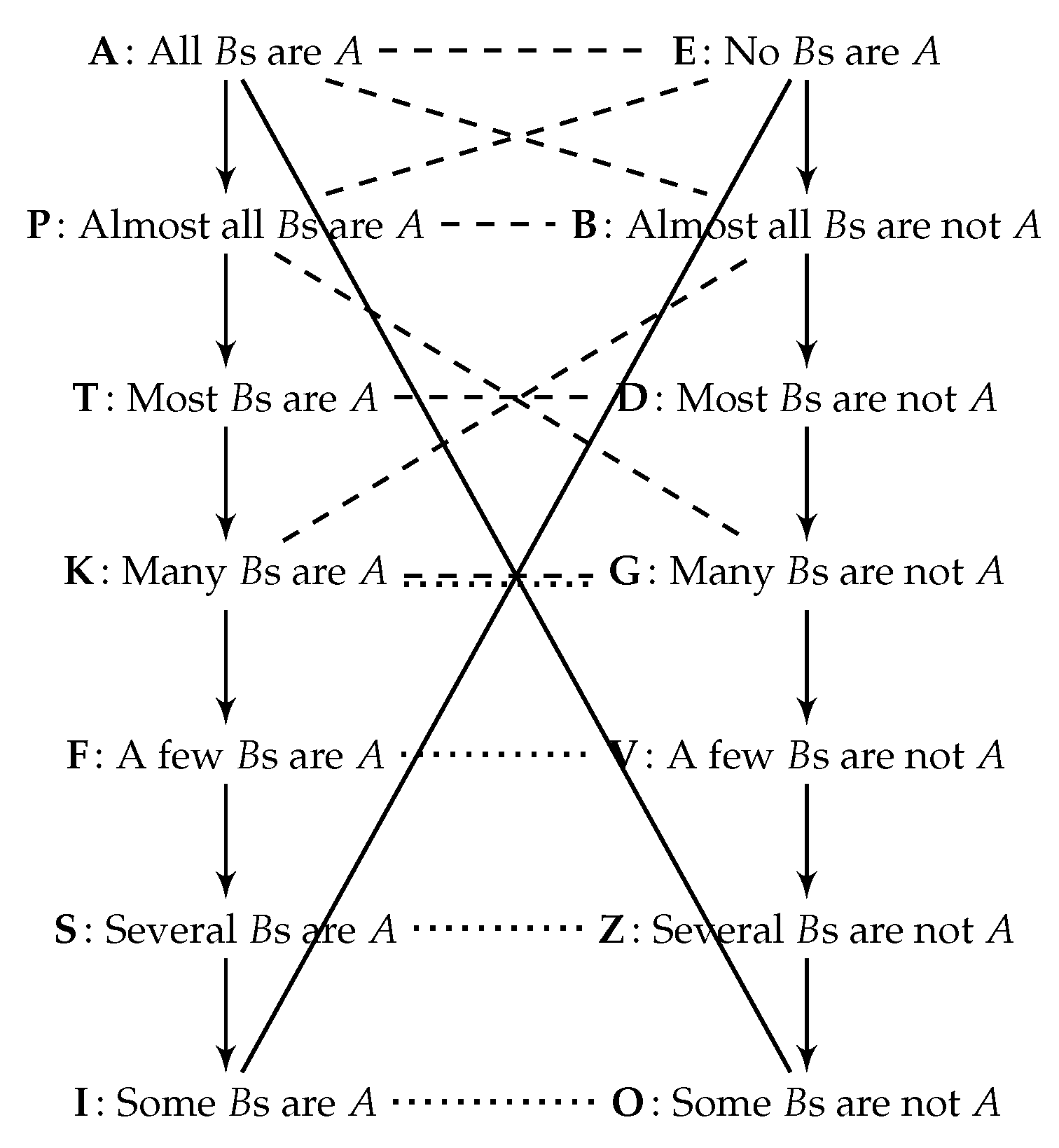
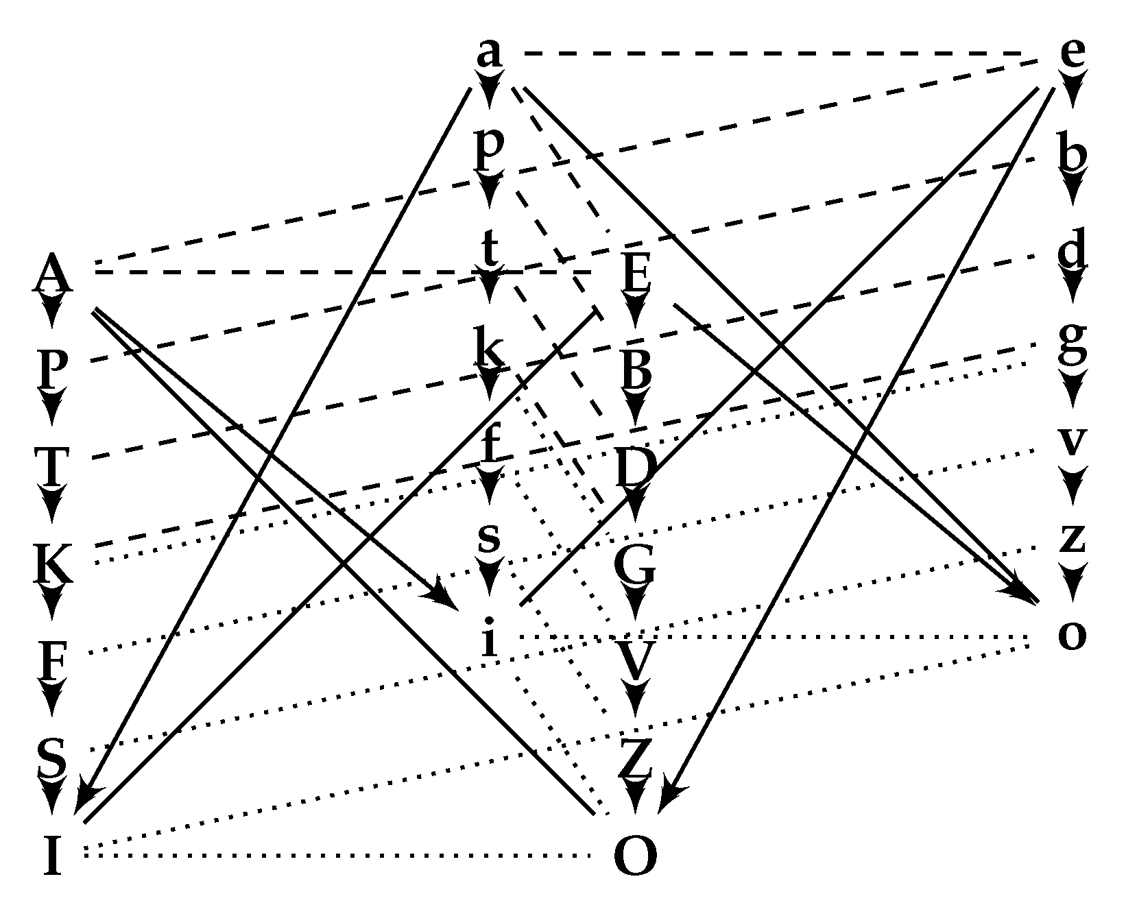
Below, we introduce the mathematical definitions of intermediate quantifiers, which form a graded Peterson’s cube of opposition (see Figure A2).

Definition 7

(New forms of fuzzy intermediate quantifiers). Let $\mathit{Ev}$ be a formula representing an evaluative expression, x be a variable, and $A,B,z$ be formulas. Then, for either of the formulas:

$$\begin{array}{cc}\hfill \left(Q_{\mathit{Ev}}^{\forall }x\right)(\mathbf{\neg }B,\mathbf{\neg }A)& \equiv (\exists z)\left[\right(\forall x\left)\right((\mathbf{\neg }B|z)x\mathbf{\Rightarrow }\mathbf{\neg }Ax)\mathbf{\wedge }\mathit{Ev}\left(\right(\mu (\mathbf{\neg }B)\left)\right(\mathbf{\neg }B\left|z\right)\left)\right],\hfill \end{array}$$

(11)

$$\begin{array}{cc}\hfill \left(Q_{\mathit{Ev}}^{\exists }x\right)(\mathbf{\neg }B,\mathbf{\neg }A)& \equiv (\exists z)\left[\right(\exists x\left)\right((\mathbf{\neg }B|z)x\mathbf{\wedge }\mathbf{\neg }Ax)\mathbf{\wedge }\mathit{Ev}\left(\right(\mu (\mathbf{\neg }B)\left)\right(\mathbf{\neg }B\left|z\right)\left)\right],\hfill \end{array}$$

(12)

either of the quantifiers (11) or (12) construes the sentence

“$\langle quantifier\rangle$ not Bs are not A”.

Below, we introduce the list of several forms of fuzzy intermediate quantifiers.

$$\begin{array}{cc}\hfill \mathbf{a}:\mathrm{All}\mathbf{\neg }B\mathrm{s}\mathrm{are}\mathrm{not}A:=& \left(Q_{\mathit{Bi}\mathbf{\Delta }}^{\forall }x\right)(\mathbf{\neg }B,\mathbf{\neg }A)\equiv (\forall x)(\mathbf{\neg }Bx\mathbf{\Rightarrow }\mathbf{\neg }Ax);\hfill \\ \hfill \mathbf{e}:\mathrm{No}\mathbf{\neg }B\mathrm{s}\mathrm{are}\mathrm{not}A:=& \left(Q_{\mathit{Bi}\mathbf{\Delta }}^{\forall }x\right)(\mathbf{\neg }B,A)\equiv (\forall x)(\mathbf{\neg }Bx\mathbf{\Rightarrow }Ax);\hfill \\ \hfill \mathbf{p}:\mathrm{Almost}\mathrm{all}\mathbf{\neg }B\mathrm{s}\mathrm{are}\mathrm{not}A:=& \left(Q_{\mathit{Bi}\mathit{Ex}}^{\forall }x\right)(\mathbf{\neg }B,\mathbf{\neg }A);\hfill \\ \hfill \mathbf{b}:\mathrm{Almost}\mathrm{all}\mathbf{\neg }B\mathrm{s}\mathrm{are}A:=& \left(Q_{\mathit{Bi}\mathit{Ex}}^{\forall }x\right)(\mathbf{\neg }B,A);\hfill \\ \hfill \mathbf{t}:\mathrm{Most}\mathbf{\neg }B\mathrm{s}\mathrm{are}\mathrm{not}A:=& \left(Q_{\mathit{Bi}\mathit{Ve}}^{\forall }x\right)(\mathbf{\neg }B,\mathbf{\neg }A);\hfill \\ \hfill \mathbf{d}:\mathrm{Most}\mathbf{\neg }B\mathrm{s}\mathrm{are}A:=& \left(Q_{\mathit{Bi}\mathit{Ve}}^{\forall }x\right)(\mathbf{\neg }B,A);\hfill \\ \hfill \mathbf{k}:\mathrm{Many}\mathbf{\neg }B\mathrm{s}\mathrm{are}\mathrm{not}A:=& \left(Q_{\mathbf{\neg }\mathit{Sm}}^{\forall }x\right)(\mathbf{\neg }B,\mathbf{\neg }A);\hfill \\ \hfill \mathbf{g}:\mathrm{Many}\mathbf{\neg }B\mathrm{s}\mathrm{are}A:=& \left(Q_{\mathbf{\neg }\mathit{Sm}}^{\forall }x\right)(\mathbf{\neg }B,A);\hfill \\ \hfill \mathbf{f}:\mathrm{A}\mathrm{few}(\mathrm{A}\mathrm{little})\mathbf{\neg }B\mathrm{s}\mathrm{are}\mathrm{not}A:=& \left(Q_{\mathit{Sm}\mathit{Si}}^{\forall }x\right)(\mathbf{\neg }B,\mathbf{\neg }A);\hfill \\ \hfill \mathbf{v}:\mathrm{A}\mathrm{few}(\mathrm{A}\mathrm{little})\mathbf{\neg }B\mathrm{s}\mathrm{are}A:=& \left(Q_{\mathit{Sm}{Si}}^{\forall }x\right)(\mathbf{\neg }B,A);\hfill \\ \hfill \mathbf{s}:\mathrm{Several}\mathbf{\neg }B\mathrm{s}\mathrm{are}\mathrm{not}A:=& \left(Q_{\mathit{Sm}\mathit{Ve}}^{\forall }x\right)(\mathbf{\neg }B,\mathbf{\neg }A);\hfill \\ \hfill \mathbf{z}:\mathrm{Several}\mathbf{\neg }B\mathrm{s}\mathrm{are}A:=& \left(Q_{\mathit{Sm}\mathit{Ve}}^{\forall }x\right)(\mathbf{\neg }B,A)\hfill \\ \hfill \mathbf{i}:\mathrm{Some}\mathbf{\neg }B\mathrm{s}\mathrm{are}\mathrm{not}A:=& \left(Q_{\mathit{Bi}\mathbf{\Delta }}^{\exists }x\right)(\mathbf{\neg }B,\mathbf{\neg }A)\equiv (\exists x)(\mathbf{\neg }Bx\mathbf{\wedge }\mathbf{\neg }Ax);\hfill \\ \hfill \mathbf{o}:\mathrm{Some}\mathbf{\neg }B\mathrm{s}\mathrm{are}A:=& \left(Q_{\mathit{Bi}\mathbf{\Delta }}^{\exists }x\right)(\mathbf{\neg }B,A)\equiv (\exists x)(\mathbf{\neg }Bx\mathbf{\wedge }Ax).\hfill \end{array}$$

If the presupposition is needed, we will denote the corresponding quantifiers by *a, *e, *p, *b, *t, *d, *k, *g, *f, *v, *s, *z, *i, and *o

Just as the theorem represents the monotonicity of the quantifiers that form Peterson’s square of opposition, we can also prove the monotonic behavior for new forms of quantifiers.

Theorem 4.

The set of implications below is provable in Ł-FTT:

1.

$\begin{array}{c}{T}^{IQ}⊢\mathit{a}\mathbf{\Rightarrow }\mathit{p},T^{IQ}⊢\mathit{p}\mathbf{\Rightarrow }\mathit{t},T^{IQ}⊢\mathit{t}\mathbf{\Rightarrow }\mathit{k},\\ T^{IQ}⊢\mathit{k}\mathbf{\Rightarrow }\mathit{f},T^{IQ}⊢\mathit{f}\mathbf{\Rightarrow }\mathit{s},T^{IQ}⊢\mathit{s}\mathbf{\Rightarrow }\mathit{i};\end{array}$

2.

$\begin{array}{c}{T}^{IQ}⊢\mathit{e}\mathbf{\Rightarrow }\mathit{b},T^{IQ}⊢\mathit{b}\mathbf{\Rightarrow }\mathit{d},T^{IQ}⊢\mathit{d}\mathbf{\Rightarrow }\mathit{g},\\ T^{IQ}⊢\mathit{g}\mathbf{\Rightarrow }\mathit{v},T^{IQ}⊢\mathit{v}\mathbf{\Rightarrow }\mathit{z},T^{IQ}⊢\mathit{z}\mathbf{\Rightarrow }\mathit{o}.\end{array}$

Proof. 

We will show the proof of $T^{IQ}⊢\mathbf{p}\mathbf{\Rightarrow }\mathbf{t}$. We know that:

$$T^{IQ}⊢(\forall x)((\mathbf{\neg }B|z)x\mathbf{\Rightarrow }\mathbf{\neg }Ax)\mathbf{\Rightarrow }(\forall x)((\mathbf{\neg }B|z)x\mathbf{\Rightarrow }\mathbf{\neg }Ax).$$

(13)

By Lemma 1, we know that $Ex\ll Ve$ and, therefore, from Theorem 1 and from (13), we obtain:

$$\begin{array}{c}{T}^{IQ}⊢[(\forall x)((\mathbf{\neg }B|z)x\mathbf{\Rightarrow }\mathbf{\neg }Ax)\mathbf{\wedge }BiEx\left(\left(\mu (\mathbf{\neg }B)\right)(\mathbf{\neg }B|z)\right)]\mathbf{\Rightarrow }\hfill \\ \hfill \mathbf{\Rightarrow }\left[\right(\forall x\left)\right((\mathbf{\neg }B|z)x\mathbf{\Rightarrow }\mathbf{\neg }Ax)\mathbf{\wedge }BiVe\left(\right(\mu (\mathbf{\neg }B)\left)\right(\mathbf{\neg }B\left|z\right)\left)\right].\end{array}$$

Then, by generalization $(\forall z)$ and the properties of the quantifiers, we obtain

$$\begin{array}{c}{T}^{IQ}⊢(\exists z)[(\forall x)((\mathbf{\neg }B|z)x\mathbf{\Rightarrow }\mathbf{\neg }Ax)\mathbf{\wedge }BiEx\left(\left(\mu (\mathbf{\neg }B)\right)(\mathbf{\neg }B|z)\right)]\mathbf{\Rightarrow }\hfill \\ \hfill \mathbf{\Rightarrow }(\exists z)\left[\right(\forall x\left)\right((\mathbf{\neg }B|z)x\mathbf{\Rightarrow }\mathbf{\neg }Ax)\mathbf{\wedge }BiVe\left(\right(\mu (\mathbf{\neg }B)\left)\right(\mathbf{\neg }B\left|z\right)\left)\right].\end{array}$$

This proof is analogous to the proof of $T^{IQ}⊢\mathbf{P}\mathbf{\Rightarrow }\mathbf{T}$ - we only replace each formula in the proof by its negation. The monotonicity of fuzzy intermediate quantifiers is ensured by the monotonicity of evaluative linguistic expressions. The other proofs of implications are similar to the proof of Theorem A2; we only replace each formula in the proof with its negation. □

There are valid forms of examples of logical syllogisms with new forms of fuzzy intermediate quantifiers related to a graded Peterson’s cube of opposition (see Appendix A).

g: Many animals which are not mammals are fish.

A: All dolphins are mammals.

o: Some animals which are not dolphins are fish.

g: Many diseases which are not lethal are virus diseases.

E: All virus diseases can not be cured by antibiotics.

i: Some diseases which can not be cured by antibiotics are not lethal diseases.

3.3. Valid Forms Related to Second Face

First, the reader is reminded of the valid syllogisms of the first figure that are related to the second face of the graded Peterson’s cube of opposition. It is not necessary to construct mathematical proofs, because the validity of syllogisms can be verified very easily by replacing individual formulas with their negations.

Theorem 5.

The following syllogisms are strongly valid in $T^{IQ}$:

aaa
aap	app
aat	apt	att
aak	apk	atk	akk
aaf	apf	atf	akf	aff
aas	aps	ats	aks	afs	ass
a(*a)i	a(*p)i	a(*t)i	a(*k)i	a(*f)i	a(*s)i	aii

Proof. 

Analogously to Theorem 2, this can be proved by replacing each formula with its negation. □

Theorem 6.

The following syllogisms are strongly valid in $T^{IQ}$:

eae
eab	epb
ead	epd	etd
eag	epg	etg	ekg
eav	epv	etv	ekv	efv
eaz	epz	etz	ekz	efz	esz
e(*a)o	e(*p)o	e(*t)o	e(*k)o	e(*f)o	e(*s)o	eio

Proof. 

Analogously to Theorem 3, this can be proved by replacing each formula by its negation. □

Similarly, we can verify the validity of other forms of logical syllogisms of the other figures. We will not repeat other figures at this point.

3.4. New Forms of Figure I

In the previous part of this paper, we showed strongly valid syllogisms of the first face and strongly valid syllogisms of the second face. Another goal of the publication is to verify the validity of logical syllogisms that describe the relationship between the first face and the second face in a graded Peterson’s cube of opposition.

Firstly we prove a strong validity of the following syllogisms by concrete syntactical proofs.

Theorem 7.

SyllogismsaEE-I, aBB-I, aDD-I, aGG-I, aVV-I, aZZ-I,andaOO-Iare strongly valid in $T^{IQ}$.

Proof. 

Let us assume the syllogism as follows:

aEE-I:	$(\forall x)(\mathbf{\neg }Mx\mathbf{\Rightarrow }\mathbf{\neg }Px)$
	$(\forall x)(Sx\mathbf{\Rightarrow }\mathbf{\neg }Mx)$
	$(\forall x)(Sx\mathbf{\Rightarrow }\mathbf{\neg }Px)$.

We know that:

$$T^{IQ}⊢(\mathbf{\neg }Mx\mathbf{\Rightarrow }\mathbf{\neg }Px)\mathbf{\Rightarrow }((Sx\mathbf{\Rightarrow }\mathbf{\neg }Mx)\mathbf{\Rightarrow }(Sx\mathbf{\Rightarrow }\mathbf{\neg }Px)).$$

By the rule of generalization of $(\forall x)$ and using the properties of the quantifiers, we have:

$$T^{IQ}⊢(\forall x)(\mathbf{\neg }Mx\mathbf{\Rightarrow }\mathbf{\neg }Px)\mathbf{\Rightarrow }((\forall x)(Sx\mathbf{\Rightarrow }\mathbf{\neg }Mx)\mathbf{\Rightarrow }(\forall x)(Sx\mathbf{\Rightarrow }\mathbf{\neg }Px)).$$

□

Proof. 

Let us assume the syllogism as follows:

aOO-I:	$(\forall x)(\mathbf{\neg }Mx\mathbf{\Rightarrow }\mathbf{\neg }Px)$
	$(\exists x)(Sx\mathbf{\wedge }\mathbf{\neg }Mx)$
	$(\exists x)(Sx\mathbf{\wedge }\mathbf{\neg }Px)$.

We know that:

$$T^{IQ}⊢(\mathbf{\neg }Mx\mathbf{\Rightarrow }\mathbf{\neg }Px)\mathbf{\Rightarrow }((Sx\mathbf{\wedge }\mathbf{\neg }Mx)\mathbf{\Rightarrow }(Sx\mathbf{\wedge }\mathbf{\neg }Px)).$$

By the rule of generalization $(\forall x)$ and using the properties of the quantifiers, we have:

$$T^{IQ}⊢(\forall x)(\mathbf{\neg }Mx\mathbf{\Rightarrow }\mathbf{\neg }Px)\mathbf{\Rightarrow }((\exists x)(Sx\mathbf{\wedge }\mathbf{\neg }Mx)\mathbf{\Rightarrow }(\exists x)(Sx\mathbf{\wedge }\mathbf{\neg }Px)).$$

□

Proof. 

Let us assume the syllogism as follows:

aBB-I:	$(\forall x)(\mathbf{\neg }Mx\mathbf{\Rightarrow }\mathbf{\neg }Px)$
	$(\exists z)\left[\right(\forall x\left)\right(\left(S\right|z)x\mathbf{\Rightarrow }\mathbf{\neg }Mx)\mathbf{\wedge }\left(BiEx\right)\left(\right(\mu S\left)\right(S\left|z\right)\left)\right]$
	$(\exists z)\left[\right(\forall x\left)\right(\left(S\right|z)x\mathbf{\Rightarrow }\mathbf{\neg }Px)\mathbf{\wedge }\left(BiEx\right)\left(\right(\mu S\left)\right(S\left|z\right)\left)\right]$.

Let us denote, by $Ev:=\left(BiEx\right)\left(\right(\mu S\left)\right(S\left|z\right))$.

We know that:

$$T^{IQ}⊢(\mathbf{\neg }Mx\mathbf{\Rightarrow }\mathbf{\neg }Px)\mathbf{\Rightarrow }\left(\left(\right(S\left|z\right)x\mathbf{\Rightarrow }\mathbf{\neg }Mx)\mathbf{\Rightarrow }(\left(S\right|z)x\mathbf{\Rightarrow }\mathbf{\neg }Px)\right).$$

By the rule of generalization $(\forall x)$ and using the properties of the quantifiers, we have:

$$T^{IQ}⊢(\forall x)(\mathbf{\neg }Mx\mathbf{\Rightarrow }\mathbf{\neg }Px)\mathbf{\Rightarrow }\left((\forall x)\left(\right(S\left|z\right)x\mathbf{\Rightarrow }\mathbf{\neg }Mx)\mathbf{\Rightarrow }((\forall x)\left(S\right|z)x\mathbf{\Rightarrow }\mathbf{\neg }Px)\right).$$

By Ł-FTT properties, we have the provable formula as follows:

$$\begin{array}{c}{T}^{IQ}⊢(\forall x)(\mathbf{\neg }Mx\mathbf{\Rightarrow }\mathbf{\neg }Px)\mathbf{\Rightarrow }\hfill \\ \hfill \mathbf{\Rightarrow }\left(\left[\right(\forall x\left)\right(\left(S\right|z)x\mathbf{\Rightarrow }\mathbf{\neg }Mx)\mathbf{\wedge }Ev]\mathbf{\Rightarrow }[(\forall x)\left(\right(S\left|z\right)x\mathbf{\Rightarrow }\mathbf{\neg }Px)\mathbf{\wedge }Ev]\right).\end{array}$$

Using the generalization rule for $(\forall z)$ and by the properties of the quantifiers we know that:

$$\begin{array}{c}{T}^{IQ}⊢(\forall x)(\mathbf{\neg }Mx\mathbf{\Rightarrow }\mathbf{\neg }Px)\mathbf{\Rightarrow }\hfill \\ \hfill \mathbf{\Rightarrow }\left((\exists z)\left[\right(\forall x\left)\right(\left(S\right|z)x\mathbf{\Rightarrow }\mathbf{\neg }Mx)\mathbf{\wedge }Ev]\mathbf{\Rightarrow }(\exists z\left)\right[(\forall x)\left(\right(S\left|z\right)x\mathbf{\Rightarrow }\mathbf{\neg }Px)\mathbf{\wedge }Ev]\right).\end{array}$$

By putting $Ev:=\left(BiEx\right)\left(\right(\mu S\left)\right(S\left|z\right))$, we obtain the strong validity of aBB-I. If we denote $Ev:=\left(BiVe\right)\left(\right(\mu S\left)\right(S\left|z\right))$, we obtain the strong validity of aDD-I. If we put $Ev:=(\mathbf{\neg }Sm)\left(\right(\mu S\left)\right(S\left|z\right))$, we have the strong validity of syllogism aGG-I. By denoting $Ev:=\left(SmSi\right)\left(\right(\mu S\left)\right(S\left|z\right))$, we obtain the strong validity of syllogism aVV-I. Finally, if we denote $Ev:=\left(SmVe\right)\left(\right(\mu S\left)\right(S\left|z\right))$, we conclude that the syllogism aZZ-I is strongly valid. □

From these strongly valid syllogisms, we can obtain other strongly valid syllogisms by using monotonicity. Below, we continue with other forms of valid syllogisms of Figure I.

Theorem 8.

Let syllogismsaEE-I, aBB-I,aDD-I,aGG-I,aVV-I,aZZ-I,aOO-I be strongly valid in $T^{IQ}$. Then, the following syllogisms are strongly valid in $T^{IQ}$:

aEE
aEB	aBB
aED	aBD	aDD
aEG	aBG	aDG	aGG
aEV	aBV	aDV	aGV	aVV
aEZ	aBZ	aDZ	aGZ	aVZ	aZZ
a(*E)O	a(*B)O	a(*D)O	a(*G)O	a(*V)O	a(*Z)O	aOO

Proof. 

From strongly valid syllogism aEE-I (Theorem 7) and from monotonicity (Theorem A2) by transitivity, we prove the strong validity of syllogisms in the first column. We prove the strong validity of syllogisms in other columns analogously. □

Theorem 9.

SyllogismsAee-I,Abb-I,Add-I,Agg-IAvv-I,Azz-I,Aoo-I are strongly valid in $T^{IQ}$.

Proof. 

Analogously to the proof of Theorem 7, this can be proved by replacing each formula by its negation. □

Theorem 10.

Let syllogismsAee-I,Abb-I,Add-I,Agg-I,Avv-I,Azz-I, andAoo-I be strongly valid in $T^{IQ}$. Then, the following syllogisms are strongly valid in $T^{IQ}$:

Aee
Aeb	Abb
Aed	Abd	Add
Aeg	Abg	Adg	Agg
Aev	Abv	Adv	Agv	Avv
Aez	Abz	Adz	Agz	Avz	Azz
A(*e)o	A(*b)o	A(*d)o	A(*g)o	A(*v)o	A(*z)o	Aoo

Proof. 

This can be proved by monotonicity (Theorem 4) similarly to Theorem 8. □

In other constructions, we will assume a selected group of valid syllogisms (these proofs can be obtained similarly as in Theorem 7), from which we will verify the validity of other forms of syllogisms, especially with the help of monotonicity. In Theorem 11 and in Theorem 12, we present other strongly valid syllogisms of Figure I.

Theorem 11.

Let syllogismsEea-I,Ebp-I,Edt-I,Egk-I,Evf-I,Ezs-I, andEoi-I be strongly valid in $T^{IQ}$. Then, the following syllogisms are strongly valid in $T^{IQ}$:

Eea
Eep	Ebp
Eet	Ebt	Edt
Eek	Ebk	Edk	Egk
Eef	Ebf	Edf	Egf	Evf
Ees	Ebs	Eds	Egs	Evs	Ezs
E(*e)i	E(*b)i	E(*d)i	E(*g)i	E(*v)i	E(*z)i	Eoi

Proof. 

This can be proved by monotonicity (Theorem 4), similarly to Theorem 8. □

Theorem 12.

Let syllogismseEA-I,eBP-I,eDT-I,eGK-I,eVF-I,eZS-I, andeOI-I be strongly valid in $T^{IQ}$. Then, the following syllogisms are strongly valid in $T^{IQ}$:

eEA
eEP	eBP
eET	eBT	eDT
eEK	eBK	eDK	eGK
eEF	eBF	eDF	eGF	eVF
eES	eBS	eDS	eGS	eVS	eZS
e(*E)I	e(*B)I	e(*D)I	e(*G)I	e(*V)I	e(*Z)I	eOI

Proof. 

This can be proved by monotonicity (Theorem A2), analogously to Theorem 8. □

We can prove other strongly valid syllogisms using the following proposition, which shows the relationship of the sub-alterns between the first and second squares of opposition.

Proposition 2

([19]). The following is provable:

(a) 

$T^{IQ}⊢\mathbf{A}\mathbf{\Rightarrow }\mathbf{i}$;

(b) 

$T^{IQ}⊢\mathbf{E}\mathbf{\Rightarrow }\mathbf{o}$;

(c) 

$T^{IQ}⊢\mathbf{a}\mathbf{\Rightarrow }\mathbf{I}$;

(d) 

$T^{IQ}⊢\mathbf{e}\mathbf{\Rightarrow }\mathbf{O}$.

Theorem 13.

Let syllogismsAAA-I,aaa-I,EAE-I,eae-I,Aee-I,aEE-I,Eea-I, andeEA-I be strongly valid in $T^{IQ}$. Then, the following syllogisms are strongly valid in $T^{IQ}$:(*A)Ai-I(*a)aI-I,(*E)Ao-I,(*e)aO-I,(*A)eO-I,(*a)Eo-I,(*E)eI-I, and(*e)Ei-I.

Proof. 

This can be proved by transitivity and by Proposition 2. □

Theorem 14.

SyllogismsoAo-I,iAi-I,oeI-I,ieO-I,IEo-I,OEi-I,IaI-I, andOaO-I are strongly valid in $T^{IQ}$.

Proof. 

Let us assume the syllogism as follows:

oAo-I:	$(\exists x)(\mathbf{\neg }Mx\mathbf{\wedge }Px)$
	$(\forall x)(Sx\mathbf{\Rightarrow }Mx)$
	$(\exists x)(\mathbf{\neg }Sx\mathbf{\wedge }Px)$.

We know that:

$$T^{IQ}⊢(Sx\mathbf{\Rightarrow }Mx)\mathbf{\Rightarrow }(\mathbf{\neg }Mx\mathbf{\Rightarrow }\mathbf{\neg }Sx).$$

We also know that:

$$T^{IQ}⊢(\mathbf{\neg }Mx\mathbf{\Rightarrow }\mathbf{\neg }Sx)\mathbf{\Rightarrow }((\mathbf{\neg }Mx\mathbf{\wedge }Px)\mathbf{\Rightarrow }(\mathbf{\neg }Sx\mathbf{\wedge }Px)).$$

By transitivity, we obtain:

$$T^{IQ}⊢(Sx\mathbf{\Rightarrow }Mx)\mathbf{\Rightarrow }((\mathbf{\neg }Mx\mathbf{\wedge }Px)\mathbf{\Rightarrow }(\mathbf{\neg }Sx\mathbf{\wedge }Px)).$$

By the rule of generalization for $(\forall x)$ and using the properties of the quantifiers, we have:

$$T^{IQ}⊢(\forall x)(Sx\mathbf{\Rightarrow }Mx)\mathbf{\Rightarrow }((\exists x)(\mathbf{\neg }Mx\mathbf{\wedge }Px)\mathbf{\Rightarrow }(\exists x)(\mathbf{\neg }Sx\mathbf{\wedge }Px)).$$

By adjunction, we obtain:

$$T^{IQ}⊢((\exists x)(\mathbf{\neg }Mx\mathbf{\wedge }Px)\mathbf{\&}(\forall x)(Sx\mathbf{\Rightarrow }Mx))\mathbf{\Rightarrow }(\exists x)(\mathbf{\neg }Sx\mathbf{\wedge }Px).$$

The strong validity of syllogism OaO-I can be proven analogously, by replacing each formula with its negation. The strong validity of other syllogisms can be proven similarly. □

Theorem 15.

Let syllogismsoAo-I,iAi-I,oeI-I,ieO-I,IEo-I,OEi-I,IaI-I, andOaO-I be strongly valid in $T^{IQ}$. Then, the following syllogisms are strongly valid in $T^{IQ}$:

(*e)Ao	(*E)aO	(*a)Ai	(*A)aI	(*e)eI	(*E)Ei	(*a)eO	(*A)Eo
(*b)Ao	(*B)aO	(*p)Ai	(*P)aI	(*b)eI	(*B)Ei	(*p)eO	(*P)Eo
(*d)Ao	(*D)aO	(*t)Ai	(*T)aI	(*d)eI	(*D)Ei	(*t)eO	(*T)Eo
(*g)Ao	(*G)aO	(*k)Ai	(*K)aI	(*g)eI	(*G)Ei	(*k)eO	(*K)Eo
(*v)Ao	(*V)aO	(*f)Ai	(*F)aI	(*v)eI	(*V)Ei	(*f)eO	(*F)Eo
(*z)Ao	(*Z)aO	(*s)Ai	(*S)aI	(*z)eI	(*Z)Ei	(*s)eO	(*S)Eo
oAo	OaO	iAi	IaI	oeI	OEi	ieO	IEo

Proof. 

By monotonicity (Theorem 4) and the strongly valid syllogism oAo-I, we prove, by transitivity, the strong validity of the syllogisms in the first column. We prove the other syllogisms in the other columns analogously by monotonicity (Theorems A2 and 4). □

3.5. New Forms of Figure II

Figure II is similar to Figure I, so we will not present concrete syntactical proofs of syllogisms. The syllogisms can be proved similarly to Theorems 7 and 14.

Theorem 16.

Let syllogismsaAA-II,aPP-II,aTT-II,aKK-II,aFF-II,aSS-II, andaII-II be strongly valid in $T^{IQ}$. Then, the following syllogisms are strongly valid in $T^{IQ}$:

aAA
aAP	aPP
aAT	aPT	aTT
aAK	aPK	aTK	aKK
aAF	aPF	aTF	aKF	aFF
aAS	aPS	aTS	aKS	aFS	aSS
a(*A)I	a(*P)I	a(*T)I	a(*K)I	a(*F)I	a(*S)I	aII

Proof. 

This can be proved by monotonicity (Theorem A2), similarly to Theorem 8. □

Theorem 17.

Let syllogismsAaa-II,App-II,Att-II,Akk-II,Aff-II,Ass-II, andAii-II be strongly valid in $T^{IQ}$. Then, the following syllogisms are strongly valid in $T^{IQ}$:

Aaa
Aap	App
Aat	Apt	Att
Aak	Apk	Atk	Akk
Aaf	Apf	Atf	Akf	Aff
Aas	Aps	Ats	Aks	Afs	Ass
A(*a)i	A(*p)i	A(*t)i	A(*k)i	A(*f)i	A(*s)i	Aii

Proof. 

This can be proved by monotonicity (Theorem 4), similarly to Theorem 8. □

Theorem 18.

Let syllogismseEA-II,eBP-II,eDT-II,eGK-II,eVF-II,eZS-II, andeOI-II be strongly valid in $T^{IQ}$. Then, the following syllogisms are strongly valid in $T^{IQ}$:

eEA
eEP	eBP
eET	eBT	eDT
eEK	eBK	eDK	eGK
eEF	eBF	eDF	eGF	eVF
eES	eBS	eDS	eGS	eVS	eZS
e(*E)I	e(*B)I	e(*D)I	e(*G)I	e(*V)I	e(*Z)I	eOI

Proof. 

This can be proved by monotonicity (Theorem A2), similarly to Theorem 8. □

Theorem 19.

Let syllogismsEea-II,Ebp-II,Edt-II,Egk-II,Evf-II,Ezs-II, andEoi-II be strongly valid in $T^{IQ}$. Then, the following syllogisms are strongly valid in $T^{IQ}$:

Eea
Eep	Ebp
Eet	Ebt	Edt
Eek	Ebk	Edk	Egk
Eef	Ebf	Edf	Egf	Evf
Ees	Ebs	Eds	Egs	Evs	Ezs
E(*e)i	E(*b)i	E(*d)i	E(*g)i	E(*v)i	E(*z)i	Eoi

Proof. 

This can be proved by monotonicity (Theorem 4), similarly to Theorem 8. □

Theorem 20.

Let syllogismsEAE-II,eae-II,AEE-II,aee-II,aAA-II,Aaa-II,Eea-II, andeEA-II be strongly valid in $T^{IQ}$. Then, the following syllogisms are strongly valid in $T^{IQ}$:(*E)Ao-II,(*e)aO-II,(*A)Eo-II,(*a)eO-II,(*a)Ai-II,(*A)aI-II,(*E)eI-II, and(*e)Ei-II.

Proof. 

This can be proved by transitivity and by Proposition 2. □

Theorem 21.

Let syllogismsOAo-II,oaO-II,IEo-II,ieO-II,OeI-II,oEi-II,IaI-II, andiAi-II be strongly valid in $T^{IQ}$. Then, the following syllogisms are strongly valid in $T^{IQ}$:

(*E)Ao	(*e)aO	(*A)Eo	(*a)eO	(*E)eI	(*e)Ei	(*a)Ai	(*A)aI
(*B)Ao	(*b)aO	(*P)Eo	(*p)eO	(*B)eI	(*b)Ei	(*p)Ai	(*P)aI
(*D)Ao	(*d)aO	(*T)Eo	(*t)eO	(*D)eI	(*d)Ei	(*t)Ai	(*T)aI
(*G)Ao	(*g)aO	(*K)Eo	(*k)eO	(*G)eI	(*g)Ei	(*k)Ai	(*K)aI
(*V)Ao	(*v)aO	(*F)Eo	(*f)eO	(*V)eI	(*v)Ei	(*f)Ai	(*F)aI
(*Z)Ao	(*z)aO	(*S)Eo	(*s)eO	(*Z)eI	(*z)Ei	(*s)Ai	(*S)aI
OAo	oaO	IEo	ieO	OeI	oEi	iAi	IaI

Proof. 

This can be proved by monotonicity (Theorems A2 and 4), analogously to Theorem 15. □

Theorem 22.

Syllogisms(*A)Ai-II,(*a)aI-II,(*E)Ei-II,(*e)eI-II,(*e)Ao-II,(*E)aO-II,(*A)eO-II, and(*a)Eo-II are strongly valid in $T^{IQ}$.

Proof. 

Let us assume the syllogism as follows:

(*A)Ai-II:	$(\forall x)(Px\mathbf{\Rightarrow }Mx)\mathbf{\&}(\exists x)(\mathbf{\neg }Mx)$
	$(\forall x)(Sx\mathbf{\Rightarrow }Mx)$
	$(\exists x)(\mathbf{\neg }Sx\mathbf{\wedge }\mathbf{\neg }Px)$.

We know that:

$$T^{IQ}⊢(Sx\mathbf{\Rightarrow }Mx)\mathbf{\Rightarrow }(\mathbf{\neg }Mx\mathbf{\Rightarrow }\mathbf{\neg }Sx).$$

(14)

We know that:

$$T^{IQ}⊢(Px\mathbf{\Rightarrow }Mx)\mathbf{\Rightarrow }(\mathbf{\neg }Mx\mathbf{\Rightarrow }\mathbf{\neg }Px).$$

(15)

We also know that:

$$T^{IQ}⊢(\mathbf{\neg }Mx\mathbf{\Rightarrow }\mathbf{\neg }Sx)\mathbf{\Rightarrow }\left((\mathbf{\neg }Mx\mathbf{\Rightarrow }\mathbf{\neg }Px)\mathbf{\Rightarrow }(\mathbf{\neg }Mx\mathbf{\Rightarrow }(\mathbf{\neg }Sx\mathbf{\wedge }\mathbf{\neg }Px\left)\right)\right).$$

(16)

By the application of transitivity on (14) and (16), we obtain:

$$T^{IQ}⊢(Sx\mathbf{\Rightarrow }Mx)\mathbf{\Rightarrow }\left((\mathbf{\neg }Mx\mathbf{\Rightarrow }\mathbf{\neg }Px)\mathbf{\Rightarrow }(\mathbf{\neg }Mx\mathbf{\Rightarrow }(\mathbf{\neg }Sx\mathbf{\wedge }\mathbf{\neg }Px\left)\right)\right).$$

By adjunction, we obtain:

$$T^{IQ}⊢(\mathbf{\neg }Mx\mathbf{\Rightarrow }\mathbf{\neg }Px)\mathbf{\Rightarrow }\left((Sx\mathbf{\Rightarrow }Mx)\mathbf{\Rightarrow }(\mathbf{\neg }Mx\mathbf{\Rightarrow }(\mathbf{\neg }Sx\mathbf{\wedge }\mathbf{\neg }Px\left)\right)\right).$$

(17)

By the application of transitivity on (15) and (17), we obtain:

$$T^{IQ}⊢(Px\mathbf{\Rightarrow }Mx)\mathbf{\Rightarrow }\left((Sx\mathbf{\Rightarrow }Mx)\mathbf{\Rightarrow }(\mathbf{\neg }Mx\mathbf{\Rightarrow }(\mathbf{\neg }Sx\mathbf{\wedge }\mathbf{\neg }Px\left)\right)\right).$$

By generalization $(\forall x)$ and the properties of the quantifiers, we obtain:

$$T^{IQ}⊢(\forall x)(Px\mathbf{\Rightarrow }Mx)\mathbf{\Rightarrow }\left((\forall x)(Sx\mathbf{\Rightarrow }Mx)\mathbf{\Rightarrow }\left(\right(\exists x)\mathbf{\neg }Mx\mathbf{\Rightarrow }(\exists x\left)\right(\mathbf{\neg }Sx\mathbf{\wedge }\mathbf{\neg }Px\left)\right)\right).$$

The strong validity of other fuzzy logical syllogisms can be verified similarly. □

3.6. New Forms of Figure III

Firstly, we will show some syntactical proofs of syllogisms on this Figure.

Theorem 23.

SyllogismsAOo-III,*(PG)o-III,*(TD)o-III,*(KB)o-III, andIEo-III are strongly valid in $T^{IQ}$.

Proof. 

Let us assume the syllogism as follows:

AOo-III:	$(\forall x)(Mx\mathbf{\Rightarrow }Px)$
	$(\exists x)(Mx\mathbf{\wedge }\mathbf{\neg }Sx)$
	$(\exists x)(\mathbf{\neg }Sx\mathbf{\wedge }Px)$.

We know that:

$$T^{IQ}⊢(Mx\mathbf{\Rightarrow }Px)\mathbf{\Rightarrow }((Mx\mathbf{\wedge }\mathbf{\neg }Sx)\mathbf{\Rightarrow }(\mathbf{\neg }Sx\mathbf{\wedge }Px)).$$

Analogously, as in previous proofs, using the properties of the quantifiers, we obtain:

$$T^{IQ}⊢(\forall x)(Mx\mathbf{\Rightarrow }Px)\mathbf{\Rightarrow }((\exists x)(Mx\mathbf{\wedge }\mathbf{\neg }Sx)\mathbf{\Rightarrow }(\exists x)(\mathbf{\neg }Sx\mathbf{\wedge }Px)).$$

□

Proof. 

Let us assume the syllogism as follows:

IEo-III:	$(\exists x)(Mx\mathbf{\wedge }Px)$
	$(\forall x)(Mx\mathbf{\Rightarrow }\mathbf{\neg }Sx)$
	$(\exists x)(\mathbf{\neg }Sx\mathbf{\wedge }Px)$.

We know that:

$$T^{IQ}⊢(Mx\mathbf{\Rightarrow }\mathbf{\neg }Sx)\mathbf{\Rightarrow }((Mx\mathbf{\wedge }Px)\mathbf{\Rightarrow }(\mathbf{\neg }Sx\mathbf{\wedge }Px)).$$

Using the generalization of $(\forall x)$ and by the logical properties of the quantifiers, we have:

$$T^{IQ}⊢(\forall x)(Mx\mathbf{\Rightarrow }\mathbf{\neg }Sx)\mathbf{\Rightarrow }((\exists x)(Mx\mathbf{\wedge }Px)\mathbf{\Rightarrow }(\exists x)(\mathbf{\neg }Sx\mathbf{\wedge }Px)).$$

By adjunction, we obtain:

$$T^{IQ}⊢(\exists x)(Mx\mathbf{\wedge }Px)\mathbf{\Rightarrow }((\forall x)(Mx\mathbf{\Rightarrow }\mathbf{\neg }Sx)\mathbf{\Rightarrow }(\exists x)(\mathbf{\neg }Sx\mathbf{\wedge }Px)).$$

□

Proof. 

Let us assume the syllogism as follows:

PGo-III:	$(\exists z)\left[\right(\forall x\left)\right(\left(M\right|z)x\mathbf{\Rightarrow }Px)\mathbf{\wedge }\left(BiEx\right)\left(\right(\mu M\left)\right(M\left|z\right)\left)\right]$
	$(\exists z^{\prime })[(\forall x)(\left(M\right|z^{\prime })x\mathbf{\Rightarrow }\mathbf{\neg }Sx)\mathbf{\wedge }(\mathbf{\neg }Sm)\left(\left(\mu M\right)\left(M\right|z^{\prime })\right)]$
	$(\exists x)(\mathbf{\neg }Sx\mathbf{\wedge }Px)$.

We know that:

$$\begin{array}{c}{T}^{IQ}⊢(\left(M\right|z)x\mathbf{\Rightarrow }Px)\mathbf{\Rightarrow }\hfill \\ \hfill \mathbf{\Rightarrow }\left((\left(M\right|z^{\prime })x\mathbf{\Rightarrow }\mathbf{\neg }Sx)\mathbf{\Rightarrow }((\left(M\right|z)x\mathbf{\&}\left(M\right|z^{\prime })x)\mathbf{\Rightarrow }(\mathbf{\neg }Sx\mathbf{\wedge }Px))\right).\end{array}$$

By generalization $(\forall x)$ and the properties of the quantifiers, we obtain:

$$\begin{array}{c}{T}^{IQ}⊢(\forall x)(\left(M\right|z)x\mathbf{\Rightarrow }Px)\mathbf{\Rightarrow }\hfill \\ \hfill \mathbf{\Rightarrow }\left((\forall x)(\left(M\right|z^{\prime })x\mathbf{\Rightarrow }\mathbf{\neg }Sx)\mathbf{\Rightarrow }((\exists x)(\left(M\right|z)x\mathbf{\&}\left(M\right|z^{\prime })x)\mathbf{\Rightarrow }(\exists x)(\mathbf{\neg }Sx\mathbf{\wedge }Px))\right).\end{array}$$

By using the property of Łukasiewicz logic, we obtain:

$$\begin{array}{c}{T}^{IQ}⊢[(\forall x)(\left(M\right|z)x\mathbf{\Rightarrow }Px)\mathbf{\wedge }Ev]\mathbf{\Rightarrow }\hfill \\ \hfill \mathbf{\Rightarrow }\left((\forall x)(\left(M\right|z^{\prime })x\mathbf{\Rightarrow }\mathbf{\neg }Sx)\mathbf{\Rightarrow }((\exists x)(\left(M\right|z)x\mathbf{\&}\left(M\right|z^{\prime })x)\mathbf{\Rightarrow }(\exists x)(\mathbf{\neg }Sx\mathbf{\wedge }Px))\right).\end{array}$$

By adjunction and the property of Łukasiewicz logic, we obtain:

$$\begin{array}{c}{T}^{IQ}⊢[(\forall x)(\left(M\right|z^{\prime })x\mathbf{\Rightarrow }\mathbf{\neg }Sx)\mathbf{\wedge }E{v}^{\prime }]\mathbf{\Rightarrow }\hfill \\ \hfill \mathbf{\Rightarrow }\left([(\forall x)(\left(M\right|z)x\mathbf{\Rightarrow }Px)\mathbf{\wedge }Ev]\mathbf{\Rightarrow }((\exists x)(\left(M\right|z)x\mathbf{\&}\left(M\right|z^{\prime })x)\mathbf{\Rightarrow }(\exists x)(\mathbf{\neg }Sx\mathbf{\wedge }Px))\right).\end{array}$$

By adjunction, we obtain:

$$\begin{array}{c}{T}^{IQ}⊢([(\forall x)(\left(M\right|z)x\mathbf{\Rightarrow }Px)\mathbf{\wedge }Ev]\mathbf{\&}[(\forall x)(\left(M\right|z^{\prime })x\mathbf{\Rightarrow }\mathbf{\neg }Sx)\mathbf{\wedge }E{v}^{\prime }]\mathbf{\&}\hfill \\ \hfill \mathbf{\&}(\exists x)(\left(M\right|z)x\mathbf{\&}\left(M\right|z^{\prime })x))\mathbf{\Rightarrow }(\exists x)(\mathbf{\neg }Sx\mathbf{\wedge }Px).\end{array}$$

By generalization $(\forall z)$, $(\forall z^{\prime })$, and the properties of the quantifiers, we obtain:

$$\begin{array}{c}{T}^{IQ}⊢(\exists z)(\exists z^{\prime })([(\forall x)(\left(M\right|z)x\mathbf{\Rightarrow }Px)\mathbf{\wedge }Ev]\mathbf{\&}[(\forall x)(\left(M\right|z^{\prime })x\mathbf{\Rightarrow }\mathbf{\neg }Sx)\mathbf{\wedge }E{v}^{\prime }]\mathbf{\&}\hfill \\ \hfill \mathbf{\&}(\exists x)(\left(M\right|z)x\mathbf{\&}\left(M\right|z^{\prime })x))\mathbf{\Rightarrow }(\exists x)(\mathbf{\neg }Sx\mathbf{\wedge }Px).\end{array}$$

If we put $Ev:=\left(BiEx\right)\left(\right(\mu M\left)\right(M\left|z\right))$ and $E{v}^{\prime }:=(\mathbf{\neg }Sm)\left(\left(\mu M\right)\left(M\right|z^{\prime })\right)$, we obtain the strong validity of syllogism *(PG)o-III. If we put $Ev:=\left(BiVe\right)\left(\right(\mu M\left)\right(M\left|z\right))$ and $E{v}^{\prime }:=\left(BiVe\right)\left(\left(\mu M\right)\left(M\right|z^{\prime })\right)$, we obtain the strong validity of syllogism *(TD)o-III. If we put $Ev:=(\mathbf{\neg }Sm)\left(\right(\mu M\left)\right(M\left|z\right))$ and $E{v}^{\prime }:=\left(BiEx\right)\left(\left(\mu M\right)\left(M\right|z^{\prime })\right)$, we obtain the strong validity of syllogism *(KB)o-III. □

Theorem 24.

Let syllogismsAOo-III,*(PG)o-III,*(TD)o-III,*(KB)o-III, andIEo-III be strongly valid in $T^{IQ}$. Then, the following syllogisms are strongly valid in $T^{IQ}$:

(*A)Eo	(*P)Eo	(*T)Eo	(*K)Eo	(*F)Eo	(*S)Eo	IEo
A(*B)o	*(PB)o	*(TB)o	*(KB)o
A(*D)o	*(PD)o	*(TD)o
A(*G)o	*(PG)o
A(*V)o
A(*Z)o
AOo

Proof. 

From the strongly valid logical syllogism AOo-III, and using the monotonicity (Theorem A2), we prove the strong validity of the syllogisms in the first column by transitivity. From the strongly valid syllogism IEo-III, and by monotonicity (Theorem A2), we can verify the strong validity of the syllogisms in the first row by transitivity. Analogously, using the strongly valid syllogism *(PG)o-III and by monotonicity (Theorem A2), we can verify the strong validity of the syllogisms in the second column by transitivity. The syllogisms in the third and the fourth column can be proven analogously. □

Theorem 25.

SyllogismsaoO-III,*(pg)O-III,*(td)O-III,*(kb)O-III, andieO-III are strongly valid in $T^{IQ}$.

Proof. 

This can be proven analogously to the proof of Theorem 23, by replacing each formula with its negation. □

Theorem 26.

Let syllogismsaoO-III,*(pg)O-III,*(td)O-III,*(kb)O-III, andieO-III be strongly valid in $T^{IQ}$. Then, the following syllogisms are strongly valid in $T^{IQ}$:

(*a)eO	(*p)eO	(*t)eO	(*k)eO	(*f)eO	(*s)eO	ieO
a(*b)O	*(pb)O	*(tb)O	*(kb)O
a(*d)O	*(pd)O	*(td)O
a(*g)O	*(pg)O
a(*v)O
a(*z)O
aoO

Proof. 

This can be proven by monotonicity (Theorem 4), similarly to Theorem 24. □

Next, we will consider the strong validity of some syllogisms without concrete proofs. These proofs are similar to the proofs in Theorem 23.

Theorem 27.

Let syllogismsEOi-III,*(BG)i-III,*(DD)i-III,*(GB)i-III, andOEi-III be strongly valid in $T^{IQ}$. Then, the following syllogisms are strongly valid in $T^{IQ}$:

E(*E)i	(*B)Ei	(*D)Ei	(*G)Ei	(*V)Ei	(*Z)Ei	OEi
E(*B)i	*(BB)i	*(DB)i	*(GB)i
E(*D)i	*(BD)i	*(DD)i
E(*G)i	*(BG)i
E(*V)i
E(*Z)i
EOi

Proof. 

This can be proven by monotonicity (Theorem A2), similarly to Theorem 24. □

Theorem 28.

Let syllogismsoeI-III,*(gb)I-III,*(dd)I-III,*(bg)I-III, andeoI-III be strongly valid in $T^{IQ}$. Then, the following syllogisms are strongly valid in $T^{IQ}$:

e(*e)I	(*b)eI	(*d)eI	(*g)eI	(*v)eI	(*z)eI	oeI
e(*b)I	*(bb)I	*(db)I	*(gb)I
e(*d)I	*(bd)I	*(dd)I
e(*g)I	*(bg)I
e(*v)I
e(*z)I
eoI

Proof. 

This can be proven by monotonicity (Theorem 4), similarly to Theorem 24. □

The following syllogisms are also strongly valid in Figure III.

Theorem 29.

Let syllogismseAe-III,EaE-III,aAa-III,AaA-III,eEA-III,Eea-III,aEE-III, andAee-III be strongly valid in $T^{IQ}$. Then, the following syllogisms are strongly valid in $T^{IQ}$:

eAe	EaE	aAa	AaA	eEA	Eea	aEE	Aee
eAb	EaB	aAp	AaP	eEP	Eep	aEB	Aeb
eAd	EaD	aAt	AaT	eET	Eet	aED	Aed
eAg	EaG	aAk	AaK	eEK	Eek	aEG	Aeg
eAv	EaV	aAf	AaF	eEF	Eef	aEV	Aev
eAz	EaZ	aAs	AaS	eES	Ees	aEZ	Aez
e(*A)o	E(*a)O	a(*A)i	A(*a)I	e(*E)I	E(*e)i	a(*E)O	A(*e)o

Proof. 

From the strongly valid syllogism eAe-III, and from monotonicity (Theorem 4), we can prove, by transitivity, the strong validity of the syllogisms in the first column. Analogously, from monotonicity (Theorems A2 and 4), we can prove the strong validity of the syllogisms in the other columns. □

Theorem 30.

Let syllogismseAe-III,EaE-III,aAa-III,AaA-III,eEA-III,Eea-III,aEE-III, andAee-III be strongly valid in $T^{IQ}$. Then, the following syllogisms are strongly valid in $T^{IQ}$:(*e)AO-III,(*E)ao-III,(*a)AI-III,(*A)ai-III,(*e)Ei-III,(*E)eI-III,(*a)Eo-III, and(*A)eO-III.

Proof. 

This can be proven by transitivity and by Proposition 2. □

3.7. New Forms of Figure IV

Firstly, we show a proof of the strongly valid syllogisms of this figure.

Theorem 31.

SyllogismsaII-IV,Aii-IV,EOi-IV,eoI-IV,aOo-IV, andAoO-IV are strongly valid in $T^{IQ}$.

Proof. 

Let us assume the syllogism as follows:

aII-IV:	$(\forall x)(\mathbf{\neg }Px\mathbf{\Rightarrow }\mathbf{\neg }Mx)$
	$(\exists x)(Mx\mathbf{\wedge }Sx)$
	$(\exists x)(Sx\mathbf{\wedge }Px)$.

We know that:

$$T^{IQ}⊢(\mathbf{\neg }Px\mathbf{\Rightarrow }\mathbf{\neg }Mx)\mathbf{\Rightarrow }(Mx\mathbf{\Rightarrow }Px).$$

(18)

We also know that:

$$T^{IQ}⊢(Mx\mathbf{\Rightarrow }Px)\mathbf{\Rightarrow }((Mx\mathbf{\wedge }Sx)\mathbf{\Rightarrow }(Sx\mathbf{\wedge }Px)).$$

(19)

By the application of transitivity on (18) and (19), we obtain:

$$T^{IQ}⊢(\mathbf{\neg }Px\mathbf{\Rightarrow }\mathbf{\neg }Mx)\mathbf{\Rightarrow }((Mx\mathbf{\wedge }Sx)\mathbf{\Rightarrow }(Sx\mathbf{\wedge }Px)).$$

By generalization $(\forall x)$ and quatifier properties, we obtain:

$$T^{IQ}⊢(\forall x)(\mathbf{\neg }Px\mathbf{\Rightarrow }\mathbf{\neg }Mx)\mathbf{\Rightarrow }((\exists x)(Mx\mathbf{\wedge }Sx)\mathbf{\Rightarrow }(\exists x)(Sx\mathbf{\wedge }Px)).$$

The strong validity of other syllogisms can be proven similarly. □

Theorem 32.

Let syllogismsaII-IV,Aii-IV,EOi-IV,eoI-IV,aOo-IV, andAoO-IV be strongly valid in $T^{IQ}$. Then, the following syllogisms are strongly valid in $T^{IQ}$:

a(*A)I	A(*a)i	E(*E)i	e(*e)I	a(*E)o	A(*e)O
a(*P)I	A(*p)i	E(*B)i	e(*b)I	a(*B)o	A(*b)O
a(*T)I	A(*t)i	E(*D)i	e(*d)I	a(*D)o	A(*d)O
a(*K)I	A(*k)i	E(*G)i	e(*g)I	a(*G)o	A(*g)O
a(*F)I	A(*f)i	E(*V)i	e(*v)I	a(*V)o	A(*v)O
a(*S)I	A(*s)i	E(*Z)i	e(*z)I	a(*Z)o	A(*z)O
aII	Aii	EOi	eoI	aOo	AoO

Proof. 

From the strongly valid syllogism aII-IV, and from monotonicity (Theorem A2), we prove the strongly valid syllogisms in the first column by transitivity. We can prove the syllogisms in the other columns analogously by using monotonicity (Theorem A2, Theorem 4). □

We will consider the strong validity of some syllogisms without concrete proofs. These proofs are similar to the previous proofs in this article.

Theorem 33.

Let syllogismsAAa-IV,aaA-IV,eAe-IV,EaE-IV,eEA-IV, andEea-IV be strongly valid in $T^{IQ}$. Then, the following syllogisms are strongly valid in $T^{IQ}$:

AAa	aaA	eAe	EaE	eEA	Eea
AAp	aaP	eAb	EaB	eEP	Eep
AAt	aaT	eAd	EaD	eET	Eet
AAk	aaK	eAg	EaG	eEK	Eek
AAf	aaF	eAv	EaV	eEF	Eef
AAs	aaS	eAz	EaZ	eES	Ees
A(*A)i	a(*a)I	e(*A)o	E(*a)O	e(*E)I	E(*e)i

Proof. 

From the strongly valid syllogism AAa-IV and monotonicity (Theorem 4), we prove, by transitivity, the strongly valid syllogism in the first column. Similarly, we can prove the strong validity of the syllogisms in the other columns by monotonicity (Theorems A2 and 4). □

Theorem 34.

Let syllogismseAe-IV,EaE-IV,eEA-IV, andEea-IV be strongly valid in $T^{IQ}$. Then, the following syllogisms are strongly valid in $T^{IQ}$:(*e)AO-IV,(*E)ao-IV,(*e)Ei-IV, and(*E)eI-IV.

Proof. 

This can be proven by transitivity and by Proposition 2. □

Theorem 35.

Let syllogismsoAO-IV,Oao-IV,oEi-IV,OeI-IV,IEo-IV, andieO-IV be strongly valid in $T^{IQ}$. Then, the following syllogisms are strongly valid in $T^{IQ}$:

(*e)AO	(*E)ao	(*e)Ei	(*E)eI	(*A)Eo	(*a)eO
(*b)AO	(*B)ao	(*b)Ei	(*B)eI	(*P)Eo	(*p)eO
(*d)AO	(*D)ao	(*d)Ei	(*D)eI	(*T)Eo	(*t)eO
(*g)AO	(*G)ao	(*g)Ei	(*G)eI	(*K)Eo	(*k)eO
(*v)AO	(*V)ao	(*v)Ei	(*V)eI	(*F)Eo	(*f)eO
(*z)AO	(*Z)ao	(*z)Ei	(*Z)eI	(*S)Eo	(*s)eO
oAO	Oao	oEi	OeI	IEo	ieO

Proof. 

From the strongly valid syllogism oAO-IV and monotonicity (Theorem 4), we prove the strongly valid syllogisms in the first column by transitivity. The syllogisms in the other columns can be proven similarly, by using monotonicity (Theorems A2 and 4). □

3.8. Examples of Logical Syllogisms in Finite Model

The model theory deals with the relation between syntax and semantics. In finite model theory, an interpretation is restricted to finite structures which have finite universes. In our examples, the models are restricted to finite universes—the universe in the first example consists of six elements and the universe in the second example consists of eight elements.

Below, we introduce several examples of new forms of logical syllogisms. We will show examples of valid syllogisms in the simple model with the finite set $M_{ϵ}$ of elements. Details of the constructed model can be found in [16]. The built model is $\mathcal{M}=\langle {(M_{\alpha },{=}_{\alpha })}_{\alpha \in Types},{\mathcal{L}}_{\Delta }\rangle$, where $M_o=[0,1]$ is based on the standard Łukasiewicz MV${}_{\Delta }$-algebra. The Łukasiewicz biresiduation ↔ represents the fuzzy equality ${=}_o$. The logical implication is represented by the Łukasiewicz residuation →.

We will assume the example of the fuzzy measure which was proposed in Section 2.3 by Equation (6). For model $\mathcal{M}$, it holds true that $\mathcal{M}\vDash T^{IQ}.$ The syllogism in model $\mathcal{M}$ is valid if

$$\mathcal{M}\left(P_1\right)\otimes \mathcal{M}\left(P_2\right)\le \mathcal{M}\left(C\right).$$

3.8.1. Example of Valid Syllogism of Figure III

Let us assume the following syllogism:

AOo:	$P_1:$ All flu are viral diseases.
	$P_2:$ Some flu are not diseases transmittable to humans
	C Some diseases which are not transmittable to humans are viral diseases.

We assume the frame which is described in the previous subsection. Let $M_{ϵ}$ be a set of diseases. We consider six diseases $U=\{u_1,u_2,u_3,u_4,u_5,u_6\}$. We interpret the formulas in the considered model as follows: Let Flu${}_{oϵ}$ be the formula “flu”, with the interpretation $\mathcal{M}\left({\mathrm{Flu}}_{oϵ}\right)=F⫇M_{ϵ}$ defined by

$$F=\{0.3/u_1,0.8/u_2,0.4/u_3,0.7/u_4,0.4/u_5,0.5/u_6\}.$$

Let Vir${}_{oϵ}$ be the formula “viral diseases”, with the interpretation $\mathcal{M}\left({\mathrm{Vir}}_{oϵ}\right)=V⫇M_{ϵ}$ defined by

$$V=\{0.8/u_1,0.2/u_2,0.3/u_3,0.9/u_4,0.7/u_5,0.6/u_6\}.$$

Let Tran${}_{oϵ}$ be the formula “diseases transmittable to humans”, with the interpretation $\mathcal{M}\left({\mathrm{Tran}}_{oϵ}\right)=T⫇M_{ϵ}$ defined by

$$T=\{0.2/u_1,0.1/u_2,0.7/u_3,0.3/u_4,0.1/u_5,0.6/u_6\}.$$

Let Ntran${}_{oϵ}$ be the formula “diseases not transmittable to humans”, with the interpretation $\mathcal{M}\left({\mathrm{Ntran}}_{oϵ}\right)=\mathbf{\neg }T⫇M_{ϵ}$ defined by

$$\mathbf{\neg }T=\{0.8/u_1,0.9/u_2,0.3/u_3,0.7/u_4,0.9/u_5,0.4/u_6\}.$$

Major premise: “All flu are viral diseases” is the formula:

$$Q_{\mathit{Bi}\mathbf{\Delta }}^{\forall }({\mathrm{Flu}}_{oϵ},{\mathrm{Vir}}_{oϵ}):=(\forall x_{ϵ})({\mathrm{Flu}}_{oϵ}\left(x_{ϵ}\right)\mathbf{\Rightarrow }{\mathrm{Vir}}_{oϵ}\left(x_{ϵ}\right)),$$

which is interpreted by:

$$\mathcal{M}\left(Q_{\mathit{Bi}\mathbf{\Delta }}^{\forall }({\mathrm{Flu}}_{oϵ},{\mathrm{Vir}}_{oϵ})\right)=\underset{m\in M_{ϵ}}{\bigwedge }(\mathcal{M}\left({\mathrm{Flu}}_{oϵ}\left(m\right)\right)\to \mathcal{M}\left({\mathrm{Vir}}_{oϵ}\left(m\right)\right))=0.4.$$

(20)

Minor premise: “Some flu are not diseases transmittable to humans” is the formula:

$$Q_{\mathit{Bi}\mathbf{\Delta }}^{\exists }({\mathrm{Flu}}_{oϵ},{\mathrm{Ntran}}_{oϵ}):=(\exists x_{ϵ})({\mathrm{Flu}}_{oϵ}\left(x_{ϵ}\right)\mathbf{\wedge }{\mathrm{Ntran}}_{oϵ}\left(x_{ϵ}\right)),$$

which is interpreted by:

$$\mathcal{M}\left(Q_{\mathit{Bi}\mathbf{\Delta }}^{\exists }({\mathrm{Flu}}_{oϵ},{\mathrm{Ntran}}_{oϵ})\right)=\underset{m\in M_{ϵ}}{\bigvee }(\mathcal{M}\left({\mathrm{Flu}}_{oϵ}\left(m\right)\right)\mathbf{\wedge }\mathcal{M}\left({\mathrm{Ntran}}_{oϵ}\left(m\right)\right))=0.8.$$

(21)

Conclusion: “Some diseases which are not transmittable to humans are viral diseases” is the formula:

$$Q_{\mathit{Bi}\mathbf{\Delta }}^{\exists }({\mathrm{Ntran}}_{oϵ},{\mathrm{Vir}}_{oϵ}):=(\exists x_{ϵ})({\mathrm{Ntran}}_{oϵ}\left(x_{ϵ}\right)\mathbf{\wedge }{\mathrm{Vir}}_{oϵ}\left(x_{ϵ}\right)),$$

which is interpreted by:

$$\mathcal{M}\left(Q_{\mathit{Bi}\mathbf{\Delta }}^{\exists }({\mathrm{Ntran}}_{oϵ},{\mathrm{Vir}}_{oϵ})\right)=\underset{m\in M_{ϵ}}{\bigvee }(\mathcal{M}\left({\mathrm{Ntran}}_{oϵ}\left(m\right)\right)\mathbf{\wedge }\mathcal{M}\left({\mathrm{Vir}}_{oϵ}\left(m\right)\right))=0.8.$$

(22)

From (20)–(22), we can see that the condition of validity in our model is satisfied because $\mathcal{M}\left(P_1\right)\otimes \mathcal{M}\left(P_2\right)=0.4\otimes 0.8=0.2\le \mathcal{M}\left(C\right)=0.8$.

3.8.2. Example of Valid Syllogism of Figure IV

(*g)Ei:	$P_1$: Many diseases which are not lethal are virus diseases.
	$P_2$: All virus diseases can not be cured by antibiotics.
	$P_3$: Some diseases which can not be cured by antibiotics are not lethal diseases.

We suppose the same frame and the fuzzy measure as in the previous example. Let $M_{ϵ}$ be a set of diseases. We consider eight diseases $V=\{v_1,v_2,v_3,v_4,v_5,v_6,v_7,v_8\}$. We interpret the formulas in the considered model as follows: Let Nlethal${}_{oϵ}$ be the formula “diseases which are not lethal”, with the interpretation $\mathcal{M}\left({\mathrm{Nlethal}}_{oϵ}\right)=\mathbf{\neg }L⫇M_{ϵ}$ defined by

$$\mathbf{\neg }L=\{1/v_1,0.8/v_2,0.3/v_3,0.5/v_4,0.7/v_5,0.4/v_6,0.4/v_7,0.4/v_8\}.$$

Let Vir${}_{oϵ}$ be the formula “virus diseases”, with the interpretation $\mathcal{M}\left({\mathrm{Vir}}_{oϵ}\right)=V⫇M_{ϵ}$ defined by

$$V=\{0.6/v_1,0.4/v_2,0.2/v_3,0.6/v_4,0.7/v_5,0.5/v_6,0.3/v_7,0.2/v_8\}.$$

Let Natb${}_{oϵ}$ be the formula “diseases which cannot be cured by antibiotics”, with the interpretation $\mathcal{M}\left({\mathrm{Natb}}_{oϵ}\right)=\mathbf{\neg }A⫇M_{ϵ}$ defined by

$$\mathbf{\neg }A=\{0.7/v_1,0.5/v_2,0.3/v_3,0.7/v_4,0.7/v_5,0.5/v_6,0.3/v_7,0.5/v_8\}.$$

Major premise: “Many diseases which are not lethal are virus diseases.” can be represented in our model as:

$$\begin{array}{c}\mathcal{M}((\exists z_{oϵ})[(\forall x_{ϵ})(\left({\mathrm{Nlethal}}_{oϵ}\right|z_{oϵ})\left(x_{ϵ}\right)\mathbf{\Rightarrow }{\mathrm{Vir}}_{oϵ}\left(x_{ϵ}\right))\mathbf{\&}\hfill \\ \hfill \mathbf{\&}(\exists x_{ϵ})\left({\mathrm{Nlethal}}_{oϵ}\right|z_{oϵ})\left(x_{ϵ}\right)\mathbf{\wedge }(\mathbf{\neg }Sm)\left(\left(\mu {\mathrm{Nlethal}}_{oϵ}\right)\left({\mathrm{Nlethal}}_{oϵ}\right|z_{oϵ})\right)\left]\right).\end{array}$$

(23)

This leads us to find the fuzzy set $\mathcal{M}$(Nlethal${}_{oϵ}\left|z_{oϵ}\right)=C⫇M_{ϵ}$, which gives us the greatest degree in (23). It can be confirmed that fuzzy set $C=\{0.5/v_4,0.7/v_5,0.4/v_6\}⫇\mathbf{\neg }L$ leads to the greatest degree in (23).

$$\mathcal{M}\left(Q_{\mathbf{\neg }\mathit{Sm}}^{\forall }({\mathrm{Nlethal}}_{oϵ},{\mathrm{Vir}}_{oϵ})\right)=1\otimes 0.7\mathbf{\wedge }1=0.7.$$

(24)

Minor premise: “All virus diseases can not be cured by antibiotics” is the formula:

$$Q_{\mathit{Bi}\mathbf{\Delta }}^{\forall }({\mathrm{Vir}}_{oϵ},{\mathrm{Natb}}_{oϵ}):=(\forall x_{ϵ})({\mathrm{Vir}}_{oϵ}\left(x_{ϵ}\right)\mathbf{\Rightarrow }{\mathrm{Natb}}_{oϵ}\left(x_{ϵ}\right)),$$

which is interpreted by:

$$\mathcal{M}\left(Q_{\mathit{Bi}\mathbf{\Delta }}^{\forall }({\mathrm{Vir}}_{oϵ},{\mathrm{Natb}}_{oϵ})\right)=\underset{m\in M_{ϵ}}{\bigwedge }(\mathcal{M}\left({\mathrm{Vir}}_{oϵ}\left(m\right)\right)\to \mathcal{M}\left({\mathrm{Natb}}_{oϵ}\left(m\right)\right))=1.$$

(25)

Conclusion: “Some diseases which can not be cured by antibiotics are not lethal diseases” is the formula:

$$Q_{\mathit{Bi}\mathbf{\Delta }}^{\exists }({\mathrm{Natb}}_{oϵ},{\mathrm{Nlethal}}_{oϵ}):=(\exists x_{ϵ})({\mathrm{Natb}}_{oϵ}\left(x_{ϵ}\right)\mathbf{\wedge }{\mathrm{Nlethal}}_{oϵ}\left(x_{ϵ}\right)),$$

which is interpreted by:

$$\mathcal{M}\left(Q_{\mathit{Bi}\mathbf{\Delta }}^{\exists }({\mathrm{Natb}}_{oϵ},{\mathrm{Nlethal}}_{oϵ})\right)=\underset{m\in M_{ϵ}}{\bigvee }(\mathcal{M}\left({\mathrm{Natb}}_{oϵ}\left(m\right)\right)\mathbf{\wedge }\mathcal{M}\left({\mathrm{Nlethal}}_{oϵ}\left(m\right)\right))=0.7.$$

(26)

From (24)–(26), we can see that the condition of validity is satisfied in our model because $\mathcal{M}\left(P_1\right)\otimes \mathcal{M}\left(P_2\right)=0.7\otimes 1=0.7\le \mathcal{M}\left(C\right)=0.7$.

4. Discussion

In the discussion section, we will comment on new forms of fuzzy syllogisms which we have proven in Section 3. In Section 3, we can see that we can order strongly valid syllogisms into triangles or columns by monotonicity. In the vertexes of these triangles are fuzzy syllogisms that consist of classical quantifiers or new forms of classical quantifiers. At the endpoints of the columns are also fuzzy syllogisms which contain classical quantifiers or new forms of classical quantifiers. Fuzzy syllogisms are proved by syntactic proofs, but we also use monotonicity to prove the strong validity of fuzzy syllogisms. We use monotonicity in three ways - to strengthen the first premise, to strengthen the second premise, or to weaken the conclusion. We also use Proposition 2 for the proofs.

4.1. Figure I

In the proofs of the strongly valid syllogisms in Theorems 8, 10, 11 and 12, we use monotonicity to weaken the conclusion. In these Theorems, we can see that we can order strongly valid syllogisms by monotonicity into triangles.

In Theorem 15, we order, by monotonicity, the strongly valid syllogisms into columns. In Theorem 15, we proved the syllogisms by strengthening the first premise.

4.2. Figure II

The structures of the syllogisms of Figure II are similar to the structures of Figure I. We use monotonicity to weaken the conclusion in the proofs of Theorems 16–19. As we can see in these Theorems that we ordered the strongly valid syllogisms into triangles by monotonicity.

In Theorem 21, we ordered the syllogisms into columns by monotonicity. In the proof, we used monotonicity to strengthen the first premise.

In Theorem 22, we can find eight strongly valid syllogisms. We showed the proof of syllogism (*A)Ai-II, in which we can see that its presupposition is a formula $(\exists x)(\mathbf{\neg }Mx)$, but the middle formula in this syllogism is $\left(Mx\right)$. This is a consequence of the property of contraposition (Lemma A1(h)). The formula representing the presupposition is related to the assumption that all formulas are not empty.

4.3. Figure III

Figure III is different than previous figures. Firstly, on this figure, we can prove non-trivial syllogisms. Non-trivial syllogisms are syllogisms, as we said in the introduction, which contain intermediate quantifiers in both premises. This group of syllogisms is specific in that valid syllogisms work with a common presupposition. While in the previous figures, it was enough to always assume the presupposition and thus the non-emptiness of the fuzzy set for one fuzzy set, for non-trivial syllogisms it is necessary to assume the non-emptiness of the fuzzy set in the antecedent in both premises. This assumption is represented by the formula below.

$$(\exists x)(\left(B\right|z)x\mathbf{\&}\left(B\right|z^{\prime })x).$$

(27)

We denote the Formula (27) as a common presupposition of existential import of two fuzzy intermediate quantifiers $\left(Q_{\mathit{Ev}}^{\forall }x\right)(B,A)$ and $\left(Q_{\mathit{Ev}}^{\forall }x\right)(B,\mathbf{\neg }A)$.

We can order strongly valid syllogisms by monotonicity into triangles. As we can see in Theorems 24 and 26–28, these triangles are oriented differently than the triangles in Figure I and Figure II. In the proofs of Theorems 24 and 26–28, we strengthen the second premise to obtain strongly valid syllogisms in the columns. To obtain the strong validity the syllogisms in the first row, we strengthen the first premise.

In Theorem 29, we can order the strongly valid syllogisms into columns by monotonicity. In this Theorem, we use monotonicity to weaken the conclusion.

4.4. Figure IV

In Figure IV, we order strongly valid syllogisms only into columns by monotonicity. We can see that in Theorem 32, we use monotonicity to strengthen the second premise. We can also see that in Theorem 33, we use monotonicity to weaken the conclusion. Finally, we can see that in Theorem 35, we use monotonicity to strengthen the first premise.

5. Conclusion and Future Work

In the article, we followed up on previous results concerning the formal proof of fuzzy logic syllogisms in fuzzy natural logic. In the introduction to the article, we first set out the motivation for this, with various references to application areas that address the issue of fuzzy generalized quantifiers. We also introduced the reader to the main mathematical territories that shape natural fuzzy logic. The main results are contained in the third section, where we first presented the mathematical definitions of fuzzy intermediate quantifiers that form a graded Peterson’s cube of opposition. We managed to formally prove, in the formal mathematical system, several new forms of logical syllogisms, the validity of which we semantically verified in the finite model. The main result is that all syntactically proven fuzzy syllogisms hold in every model.

We see further development of this article in two directions. We will first focus on extending the structure of valid fuzzy logical syllogisms by more premises. In the second part, we would like to mathematically propose Peterson’s rules of distributivity, quality, and quantity for verifying the validity of logical syllogisms related to a graded Peterson’s cube of opposition. The second main objective for the future is to program an algorithm based on these rules and verify the validity of new forms of fuzzy syllogisms automatically.

References

1. Kulicki, P. Aristotle’s Syllogistic as a Deductive System. Axioms 2020, 9, 56. [Google Scholar] [CrossRef]
2. Castro-Manzano, J.M. Traditional Logic and Computational Thinking. Philosophies 2021, 6, 12. [Google Scholar] [CrossRef]
3. Alvarez-Fontecilla, E.; Lungenstrass, T. Aristotelian Logic Axioms in Propositional Logic. Pouch Method Hist. Philos. Log. 2019, 40, 12–21. [Google Scholar] [CrossRef]
4. Alvarez, E.; Correia, M. Syllogistic with Indefinite Terms. Hist. Philos. Log. 2012, 33, 297–306. [Google Scholar] [CrossRef]
5. Knachel, M. Categorical Syllogisms. 2019. Available online: https://www.youtube.com/watch?v=80PoPICR1DU (accessed on 2 July 2019).
6. Mostowski, A. On a Generalization of Quantifiers. Fundam. Math. 1957, 44, 12–36. [Google Scholar] [CrossRef]
7. Peterson, P. Intermediate Quantifiers. Logic, linguistics, and Aristotelian semantics; Ashgate: Aldershot, UK, 2000. [Google Scholar]
8. Peterson, P. On the logic of “Few”, “Many” and “Most”. Notre Dame J. Form. Log. 1979, 20, 155–179. [Google Scholar] [CrossRef]
9. Thompson, B.E. Syllogisms using “Few”, “Many” and “Most”. Notre Dame J. Form. Log. 1982, 23, 75–84. [Google Scholar] [CrossRef]
10. Zadeh, L.A. A computational approach to fuzzy quantifiers in natural languages. Comput. Math. 1983, 9, 149–184. [Google Scholar] [CrossRef] [Green Version]
11. Dubois, D.; Prade, H. On fuzzy syllogisms. Comput. Intell. 1988, 4, 171–179. [Google Scholar] [CrossRef]
12. Dubois, D.; Godo, L.; López de Mántras, R.; Prade, H. Qualitative Reasoning with Imprecise Probabilities. J. Intell. Inf. Syst. 1993, 2, 319–363. [Google Scholar] [CrossRef]
13. Pereira-Fariña, M.; Díaz-Hermida, F.; Bugarín, A. On the analysis of set-based fuzzy quantified reasoning using classical syllogistics. Fuzzy Sets Syst. 2013, 214, 83–94. [Google Scholar] [CrossRef] [Green Version]
14. Delgado, M.; Ruiz, M.; Sánchez, D.; Vila, M.A. Fuzzy quantification:a state of the art. Fuzzy Sets Syst. 2014, 242, 1–30. [Google Scholar] [CrossRef]
15. Pereira-Fariña, M.; Vidal, J.C.; Díaz-Hermida, F.; Bugarín, A. A fuzzy syllogistic reasoning schema for generalized quantifiers. Fuzzy Sets Syst. 2014, 234, 79–96. [Google Scholar] [CrossRef] [Green Version]
16. Novák, V. A Formal Theory of Intermediate Quantifiers. Fuzzy Sets Syst. 2008, 159, 1229–1246. [Google Scholar] [CrossRef]
17. Novák, V. A Comprehensive Theory of Trichotomous Evaluative Linguistic Expressions. Fuzzy Sets Syst. 2008, 159, 2939–2969. [Google Scholar] [CrossRef] [Green Version]
18. Murinová, P.; Novák, V. The structure of generalized intermediate syllogisms. Fuzzy Sets Syst. 2014, 247, 18–37. [Google Scholar] [CrossRef]
19. Murinová, P. Graded Structures of Opposition in Fuzzy Natural Logic. Log. Universalis 2020, 265, 495–522. [Google Scholar] [CrossRef]
20. Novák, V. Linguistic characterization of time series. Fuzzy Sets Syst. 2015, 285, 52–72. [Google Scholar] [CrossRef]
21. Kacprzyk, J.; Wilbik, A.; Zadrozny, S. Linguistic summarization of time series using a fuzzy quantifier driven aggregation. Fuzzy Sets Syst. 2008, 159, 1485–1499. [Google Scholar] [CrossRef]
22. Kacprzyk, J.; Zadrożny, S. Linguistic database summaries and their protoforms: Towards natural language based knowledge discovery tools. Inf. Sci. 2005, 173, 281–304. [Google Scholar] [CrossRef]
23. Yager, R. A new approach to the summarization of data. Inf. Sci. 1982, 28, 69–86. [Google Scholar] [CrossRef]
24. Yager, R. On ordered weighted averaging operators in multicriteria decision making. IEEE Trans. Syst. Man Cybern 1988, 18, 182–190. [Google Scholar] [CrossRef]
25. Yager, R. On linguistic summaries of data. In Knowledge Discovery in Databases; Piatetsky-Shapiro, G., Frawley, W.J., Eds.; AAAI MIT Press: Cambridge, MA, USA, 1991; pp. 347–363. [Google Scholar]
26. Yager, R. Linguistic summaries as a tool for database discovery. In Proceedings of the FUZZIEEE 1995 Workshop on Fuzzy Database Systems and Information Retrieval, Yokohama, Japan, 20–21 March 1995; pp. 79–82. [Google Scholar]
27. Kacprzyk, J.; Yager, R. Linguistic summaries of data using fuzzy logic. Int. J. Gen. Syst. 2001, 30, 133–154. [Google Scholar] [CrossRef]
28. Kacprzyk, J.; Zadrożny, S. Linguistic summarization of data sets using association rules. In Proceedings of the FUZZ-IEE’03, St. Louis, MO, USA, 25–28 May 2003; pp. 702–707. [Google Scholar]
29. Wilbik, A.; Kaymak, U. Linguistic Summarization of Processes—A research agenda. In Proceedings of the 2015 Conference of the International Fuzzy Systems Association and the European Society for Fuzzy Logic and Technology, Gijon, Spain, 30 June–3 July 2015; pp. 136–143. [Google Scholar]
30. Murinová, P.; Burda, M.; Pavliska, V. An algorithm for Intermediate Quantifiers and the Graded Square of Opposition towards Linguistic Description of Data. In Advances in Fuzzy Logic and Technology; Springer: Cham, Switzerland, 2017; pp. 592–603. [Google Scholar]
31. Novák, V.; Perfilieva, I.; Dvořák, A. Insight into Fuzzy Modeling; Wiley & Sons: Hoboken, NJ, USA, 2016. [Google Scholar]
32. Novák, V. On Fuzzy Type Theory. Fuzzy Sets Syst. 2005, 149, 235–273. [Google Scholar] [CrossRef]
33. Cignoli, R.L.O.; D’Ottaviano, I.M.L.; Mundici, D. Algebraic Foundations of Many-Valued Reasoning; Kluwer: Dordrecht, The Netherlands, 2000. [Google Scholar]
34. Novák, V.; Perfilieva, I.; Močkoř, J. Mathematical Principles of Fuzzy Logic; Kluwer: Boston, MA, USA, 1999. [Google Scholar]
35. Andrews, P. An Introduction to Mathematical Logic and Type Theory: To Truth through Proof; Kluwer: Dordrecht, The Netherlands, 2002. [Google Scholar]
36. Dubois, D.; Prade, H.; Rico, A. Structures of Opposition and Comparisons: Boolean and Gradual Cases. Log. Universalis 2020, 14, 115–149. [Google Scholar] [CrossRef]
37. Dubois, D.; Prade, H.; Rico, A. Graded cubes of opposition and possibility theory with fuzzy events. Int. J. Approx. Reason. 2017, 84, 168–185. [Google Scholar] [CrossRef] [Green Version]
Publisher’s Note: MDPI stays neutral with regard to jurisdictional claims in published maps and institutional affiliations.