A Novel βSA Ensemble Model for Forecasting the Number of Confirmed COVID-19 Cases in the US

Abstract

In December 2019, Severe Special Infectious Pneumonia (SARS-CoV-2)–the novel coronavirus (COVID-19)– appeared for the first time, breaking out in Wuhan, China, and the epidemic spread quickly to the world in a very short period time. According to WHO data, ten million people have been infected, and more than one million people have died; moreover, the economy has also been severely hit. In an outbreak of an epidemic, people are concerned about the final number of infections. Therefore, effectively predicting the number of confirmed cases in the future can provide a reference for decision-makers to make decisions and avoid the spread of deadly epidemics. In recent years, the α-Sutte indicator method is an excellent predictor in short-term forecasting; however, the α-Sutte indicator uses fixed static weights. In this study, by adding an error-based dynamic weighting method, a novel β-Sutte indicator is proposed. Combined with ARIMA as an ensemble model (βSA), the forecasting of the future COVID-19 daily cumulative number of cases and the number of new cases in the US are evaluated from the experiment. The experimental results show that the forecasting accuracy of βSA proposed in this study is better than other methods in forecasting with metrics MAPE and RMSE. It proves the feasibility of adding error-based dynamic weights in the β-Sutte indicator in the area of forecasting.

1. Introduction

In December 2019, Severe Special Infectious Pneumonia (SARS-CoV-2)–the novel coronavirus (COVID-19)–appeared for the first time, breaking out in Wuhan City, Hubei Province, China. To curb the spread of the epidemic, the Chinese government authorities imposed a lockdown policy on Wuhan; however, the virus had already spread to all continents through the global transportation industry. According to the World Health Organization (WHO), COVID-19 is an emerging disease which has the characteristics of human-to-human transmission and is extremely contagious, can infect ten million people, and has caused more than millions of deaths around the world. Due to the impact of COVID-19 on people’s lives, the general public and the government are concerned about how many people will eventually be infected [1]. Many academics have invested in research on COVID-19, for example, to predict the future daily and monthly number forecasting of confirmed cases [2,3,4], or to discover related factors that affect the severity of the epidemic and cause death [5,6].

The cumulative number of confirmed COVID-19 cases in the United States is ranked No. 1 in the world, and the total number of confirmed cases accounted for 20% of global infections (https://covid19.who.int/, accessed on 10 July 2021). The U.S. is the country with the most COVID-19 confirmed cases in the world. If we can correctly predict the number of confirmed cases in the U.S., then we can know the future trend of confirmed COVID-19 cases of the world.

Forecasting methods deal with uncertainties about the future, which is crucial in helping decision-makers to make reasonable decisions and plan activities. In various fields of society, effective and highly accurate forecasts are considered important prerequisites for the effective management of an organization [7].

In recent years, the α-Sutte indicator method [8] has been an excellent predictor in short-term forecasting; however, the α-Sutte indicator uses fixed static weights. To improve the forecasting accuracy, adding weights to unweighted models is usually better than the original unweighted ones. Al-Dahidi, Baraldi, Zio, and Legnani [9] have proven that adding dynamic weights to the ensemble model led to better results than the original. Since the α-Sutte indicator uses static weight in forecasting, this study attempts to add dynamic weights into the α-Sutte indicator and incorporate it with the ARIMA method to make an ensemble forecasting model. The forecasting targets are the daily cumulative number of confirmed COVID-19 cases and the number of new COVID-19 cases in the US, and the five worst-hit states with the largest number of cumulative confirmed cases are also included for evaluation. It is hoped that the results of this study can help to make up for the lack of diversity issue in previous COVID-19 related research.

The rest of the paper is sectioned as follows. Section 2 is the improved β-Sutte indicator and βSA Ensemble model based on the α-Sutte indicator. Section 3 is the experimental process and model evaluation metrics. Section 4 predicts the results and discussion one day and five days ahead, leading finally, to the conclusion.

2. Materials and Methods

2.1. Data Collection

The data source of this study is adopted from the Centers for Disease Control and Prevention (CDC) in the United States (https://covid.cdc.gov/covid-data-tracker/ accessed on 10 July 2021). The variables and definitions of the dataset are shown in

Table 1. Variables and definitions.

Variables	Definitions
submission_date	Date
state	U.S. State Name
tot_cases	Total number of cases
conf_cases	Total number of confirmed cases
prob_cases	Possible total number of cases
new_case	Number of new confirmed cases
pnew_case	Number of new possible cases
tot_death	Total number of deaths
conf_death	Total number of confirmed deaths
prob_death	Total number of possible deaths
new_death	Number of newly confirmed deaths
pnew_death	Number of new possible death cases
created_at	Date of the profile created
consent_cases	If agreed, include confirmed and possible cases. If disagreed, only include all cases
consent_deaths	If agreed, it includes confirmed and possible deaths. If disagreed, only all deaths are included.

.

Since the dataset does not provide the daily cumulative number of confirmed cases and the number of new cases in the U.S., and there are missing values in the daily cumulative number of confirmed cases in each state of the United States in the dataset, this study adds up the cumulative number of confirmed cases (conf_cases) and the number of new cases (new_case) in each state in the United States. The five worst-hit states in the cumulative number of confirmed cases are selected for evaluation.

2.2. The α-Sutte and Proposed β-Sutte Indicator

Definitions and descriptions of notations in this study are shown in

Table 2. Notation of symbols.

Notations	Definition
$d\left(t\right)$	Observation at the t-th day
$d\left(t-k\right)$	$\mathrm{Observation} \mathrm{at} \left(t-k\right)th$ day
$D_i, \tilde{d}\left(t\right)$	The forecasting value at the $t$-th day
$\delta \left(t\right), \delta$	$\mathrm{Define} \mathrm{as} \mathrm{the} \mathrm{observation} \mathrm{of} d\left(t-4\right)$
$\alpha \left(t\right), \alpha$	$\mathrm{Define} \mathrm{as} \mathrm{the} \mathrm{observation} \mathrm{of} d\left(t-3\right)$
$\beta \left(t\right), \beta$	$\mathrm{Define} \mathrm{as} \mathrm{the} \mathrm{observation} \mathrm{of} d\left(t-2\right)$
$\gamma \left(t\right), \gamma$	$\mathrm{Define} \mathrm{as} \mathrm{the} \mathrm{observation} \mathrm{of} d\left(t-1\right)$
$\Delta x\left(t\right), \Delta x$	$\mathrm{Define} \mathrm{as} \mathrm{the} \mathrm{difference} \mathrm{of} \alpha \left(t\right)-\delta \left(t\right)$
$\Delta y\left(t\right), \Delta y$	$\mathrm{Define} \mathrm{as} \mathrm{the} \mathrm{difference} \mathrm{of} \beta \left(t\right)-\alpha \left(t\right)$
$\Delta z\left(t\right), \Delta z$	$\mathrm{Define} \mathrm{as} \mathrm{the} \mathrm{difference} \mathrm{of} \gamma \left(t\right)-\beta \left(t\right)$
${\mathsf{\epsilon }}_a\left(t\right), {\mathsf{\epsilon }}_b\left(t\right), {\mathsf{\epsilon }}_g\left(t\right)$	Error function
${\mathsf{\omega }}_a\left(t\right), {\mathsf{\omega }}_b\left(t\right), {\mathsf{\omega }}_g\left(t\right)$	The dynamic weighting function

.

The α-Sutte indicator was proposed in 2017, and it can be used to predict a variety of different time-series data [8]. During the forecasting process, the α-Sutte indicator only uses previous four data points ($\gamma , \beta , \alpha , \delta$) to make a next point forecasting, therefore, it is flexible when using any type of data [8]. The equation of the α-Sutte indicator is shown in Equation (1):

$$D_i=\frac{\alpha \left[\frac{\mathsf{\Delta }x}{\frac{\alpha +\delta }{2}}\right]+\beta \left[\frac{\mathsf{\Delta }y}{\frac{\beta +\alpha }{2}}\right]+\gamma \left[\frac{\mathsf{\Delta }z}{\frac{\gamma +\beta }{2}}\right]}{3}$$

(1)

As can be seen in Equation (1), the α-Sutte indicator divides static weight, which is 1/3, into three different error items to make the final forecasting. In this study, a novel forecasting indicator which uses dynamic weighting, the β-Sutte indicator, is proposed.

To ensure the clarity of our proposed β-Sutte indicator, $a\left(t\right), b\left(t\right), g\left(t\right)$ are defined as:

$$a\left(t\right)=\alpha \left(t\right)\left[\frac{\mathsf{\Delta }x\left(t\right)}{\frac{\alpha \left(t\right)+\delta \left(t\right)}{2}}\right]$$

$$b\left(t\right)=\beta \left(t\right)\left[\frac{\mathsf{\Delta }y\left(t\right)}{\frac{\beta \left(t\right)+\alpha \left(t\right)}{2}}\right]$$

$$g\left(t\right)=\gamma \left(t\right)\left[\frac{\mathsf{\Delta }z\left(t\right)}{\frac{\gamma \left(t\right)+\beta \left(t\right)}{2}}\right]$$

Abdollahi and Ebrahimi [10] used average weights, a weighting method based on error value, and a genetic algorithm to assign weights to three different methods in an ensemble model, pointing out that the result of the ensemble model using genetic algorithm is the best, the second best is the weighting method based on the error value, and the average weight is the worst-performing. Abdollahi and Ebrahimi [10] believe that a large part of the success of the model they put forward depends on the choice of weighting method. Based on the calculation time and cost issues, the authors of this study believe that the weighting method based on the error value used by Abdollahi and Ebrahimi [10] is an effective method to improve the forecasting accuracy without excessive cost; the principle is that method produces a higher error will be assigned a smaller weight. The dynamic weighting functions are obtained from the average of three different time estimated errors of $a\left(t\right), b\left(t\right), \mathrm{and} g\left(t\right)$ which are at day t-1, t-2, and t-3. Therefore, the dynamic weighting functions of our proposed β-Sutte indicator are defined as follows:

$${\mathsf{\omega }}_a\left(t\right)=\frac{\frac{1}{{\mathsf{\epsilon }}_a\left(t\right)}}{{{\displaystyle \sum }}_{j=1}^3 \frac{1}{{\mathsf{\epsilon }}_j\left(t\right)}}$$

$${\mathsf{\omega }}_b\left(t\right)=\frac{\frac{1}{{\mathsf{\epsilon }}_b\left(t\right)}}{{{\displaystyle \sum }}_{j=1}^3 \frac{1}{{\mathsf{\epsilon }}_j\left(t\right)}}$$

$${\mathsf{\omega }}_g\left(t\right)=\frac{\frac{1}{{\mathsf{\epsilon }}_g\left(t\right)}}{{{\displaystyle \sum }}_{j=1}^3 \frac{1}{{\mathsf{\epsilon }}_j\left(t\right)}}$$

where

$${\mathsf{\epsilon }}_a\left(t\right)=\frac{\left|d\left(t-3\right)-a\left(t-3\right)\right|+\left|d\left(t-2\right)-a\left(t-2\right)\right|+\left|d\left(t-1\right)-a\left(t-1\right)\right|}{3}$$

$${\mathsf{\epsilon }}_b\left(t\right)=\frac{\left|d\left(t-3\right)-b\left(t-3\right)\right|+\left|d\left(t-2\right)-b\left(t-2\right)\right|+\left|d\left(t-1\right)-b\left(t-1\right)\right|}{3}$$

$${\mathsf{\epsilon }}_g\left(t\right)=\frac{\left|d\left(t-3\right)-g\left(t-3\right)\right|+\left|d\left(t-2\right)-g\left(t-2\right)\right|+\left|d\left(t-1\right)-g\left(t-1\right)\right|}{3}$$

and

$${\displaystyle \sum }_{j=1}^3 \frac{1}{{\mathsf{\epsilon }}_j\left(t\right)}=\frac{1}{{\mathsf{\epsilon }}_a\left(t\right)}+\frac{1}{{\mathsf{\epsilon }}_b\left(t\right)}+\frac{1}{{\mathsf{\epsilon }}_g\left(t\right)}$$

Then, our proposed β-Sutte indicator of forecasting is shown in Equation (2):

$$\tilde{d}\left(t\right)={\mathsf{\omega }}_a\left(t\right) · a\left(t\right)+{\mathsf{\omega }}_b\left(t\right) · b\left(t\right)+{\mathsf{\omega }}_g\left(t\right) · g\left(t\right)$$

(2)

2.3. Autoregressive Integrated Moving Average (ARIMA)

The autoregressive integrated moving average (ARIMA) model was introduced by George Box and Gwilym Jenkins in 1976. The model of ARIMA is generally written with notation ARIMA (p, d, q), with p representing the order of the autoregressive (AR) process, d representing the differencing, and q stating the order of the moving average (MA) process.

Abolmaali & Shirzaei [11] have compared the results of different models (SIR Model, linear regression, logistic function, ARIMA) in the prediction of confirmed COVID-19 cases in 2021. Although the linear regression model performs well in short-term prediction, overall, the ARIMA model is still better than other models. Therefore, we chose the ARIMA model to compare with our proposed β-Sutte indicator and βSA ensemble model.

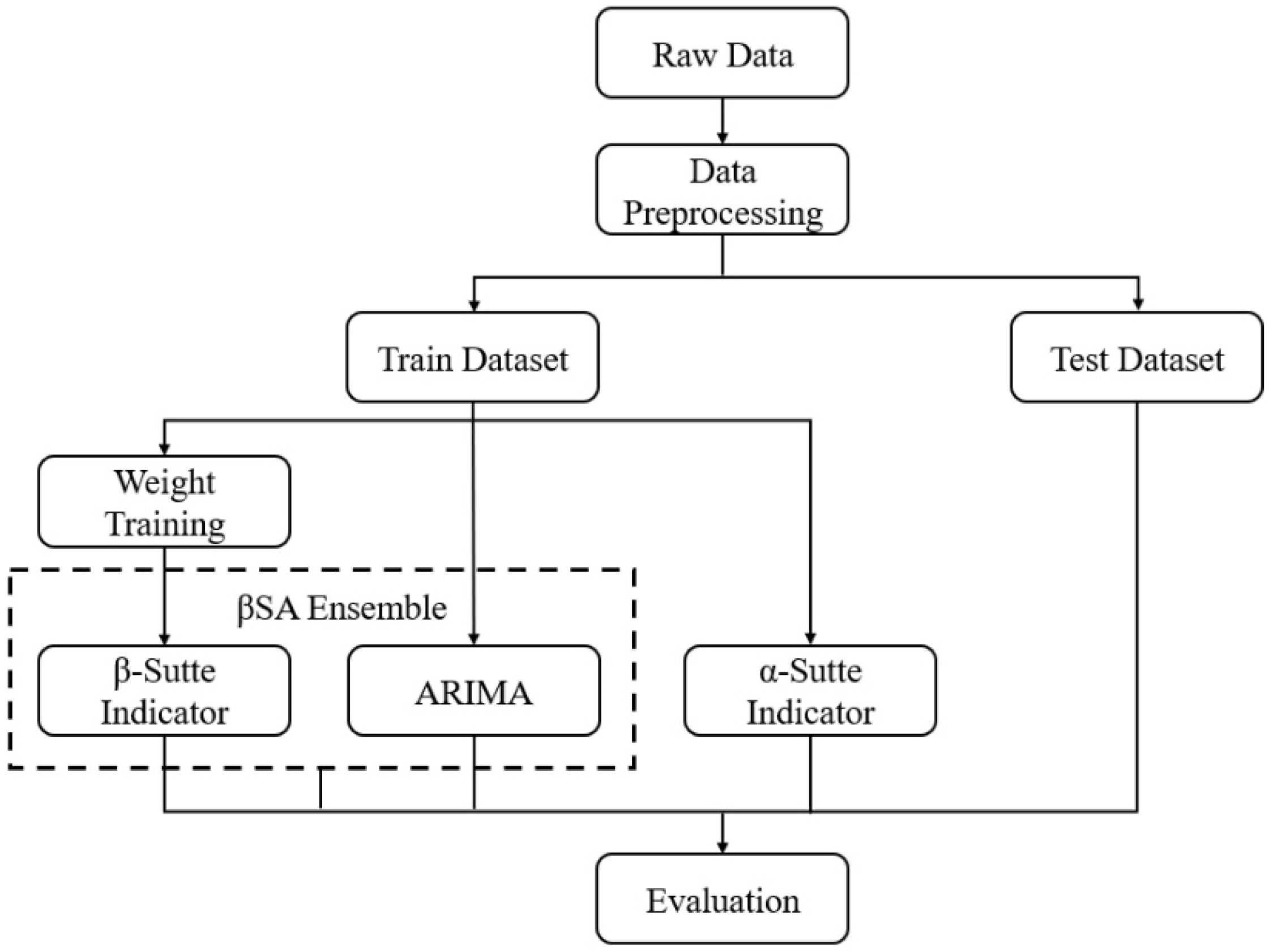
2.4. βSA Ensemble Model

The βSA Ensemble model is mainly based on the SutteARIMA prediction method proposed by Ahmar & Del Val [12]. SutteARIMA combines α-Sutte indicator and ARIMA; as such, the prediction result of SutteARIMA is the average of α-Sutte indicator and ARIMA. In terms of prediction results, SutteARIMA is better than ARIMA, but the results are quite close. The proposed βSA ensemble model tries to combine the proposed β-Sutte indicator with ARIMA, and the prediction result of the βSA ensemble model is the average of the two prediction results.

3. Experiment

3.1. Data

Data regarding confirmed US COVID-19 cases were obtained from the Centers for Disease Control and Prevention (CDC) in the United States. Due to the large number of vaccines used in the United States after July 2021, only data from 25 July 2020 to 30 June 2021 are used for method evaluation. This study proposes an improved β-Sutte indicator and βSA ensemble model based on the α-Sutte indicator to forecast the cumulative number of confirmed cases and the daily number of newly confirmed cases of COVID-19 in the U.S. in different forecast periods (over one day and five days). It is expected to outperform the α-Sutte indicator and ARIMA on model evaluation metrics.

3.2. Metrics

For the evaluation of the forecasting methods, we applied two forecasting accuracy measures, including mean absolute percentage error (MAPE) and root mean square error (RMSE) [13]. The indicators of both measures are the smaller the better.

MAPE and RMSE are defined as follows:

Assuming $\overline{y}$ are the predicted values, and y are real values:

$$\overline{y}=\left\{\overline{y_1}, \overline{y_2, }\cdots , \overline{y_n}\right\}, y=\left\{y_1, y_2, \cdots , y_n\right\}$$

$$\mathrm{MAPE}=\frac{100\%}{n}{{\displaystyle \sum }}_{i=1}^n\left|\frac{\overline{y_i}-y_i}{y_i}\right|$$

(3)

$$\mathrm{RMSE}=\sqrt{\frac{1}{n}{{\displaystyle \sum }}_{i=1}^n{\left(\overline{y_i}-y_i\right)}^2}$$

(4)

MAPE and RMSE metrics are used for evaluating the quality of the model, and their values will vary between 0 and infinity. MAPE focuses on percentage errors, while RMSE is more sensitive to the data structure (numerical units, outliers). Both of these metrics are as small as possible, but there is no absolute reference value [14]. The results of this forecasting were obtained by using R Software with the forecast and SutteForecastR Package.

3.3. Flow Chart of Experiment

This section will give a detailed description of the experiment process in this study, including data pre-processing, dataset split, weight training, the α-Sutte indicator, the β-Sutte indicator, ARIMA, and βSA. The evaluation flow chart is shown in Figure 1.

The detailed experiment process is as follows:

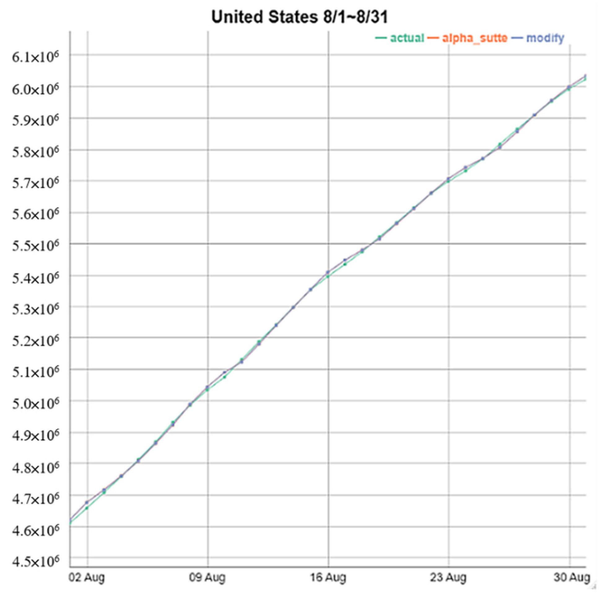
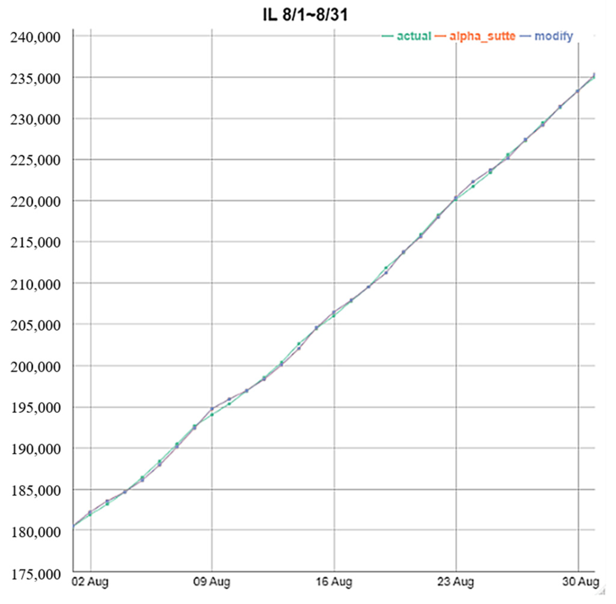
• The data set used in this study does not provide the daily cumulative total number of confirmed cases in the U.S., Therefore, this study applies to sum up the daily cumulative total number of cases (tot_cases) of all states to calculate the daily cumulative total number of confirmed cases in the U.S. In addition, it will select the five worst-hit states of the cumulative number of confirmed cases for evaluation.
• Split the preprocessed data set into training days from $d\left(t-7\right)$ to $d\left(t-1\right)$ and a testing day $d\left(t\right)$. The time window is set to eight, and the sliding window is set to one.
• Employ the dynamic weighting method based on the error value, and calculate the training weights ${\mathsf{\omega }}_a\left(t\right)$, ${\mathsf{\omega }}_b\left(t\right)$,${\mathsf{\omega }}_g\left(t\right)$ according to their error function ${\mathsf{\epsilon }}_a\left(t\right)$, ${\mathsf{\epsilon }}_b\left(t\right)$, ${\mathsf{\epsilon }}_g\left(t\right)$.
• By using the sliding window method to obtain the moving dynamic weights, the time points of training days required for the β-Sutte indicator is seven. Let the obtained dynamic weights be incorporated into the β-Sutte indicator to predict $\tilde{d}\left(t\right).$
• The ARIMA method uses the same dataset, then averages the results of β-Sutte indicator and ARIMA, becoming the final result of the βSA ensemble model. In addition, α-Sutte indicator is also used to compare other models with different forecast periods (one-day-ahead and five days ahead, respectively).
• Compare and discuss the results of different methods (α-Sutte indicator, β-Sutte indicator, ARIMA, and βSA ensemble model) by using evaluation metrics with RMSE and MAPE. It is expected that the β-Sutte indicator and the βSA ensemble model are better than the α-Sutte indicator and ARIMA in the performance of model evaluation metrics.

4. Results and Discussion

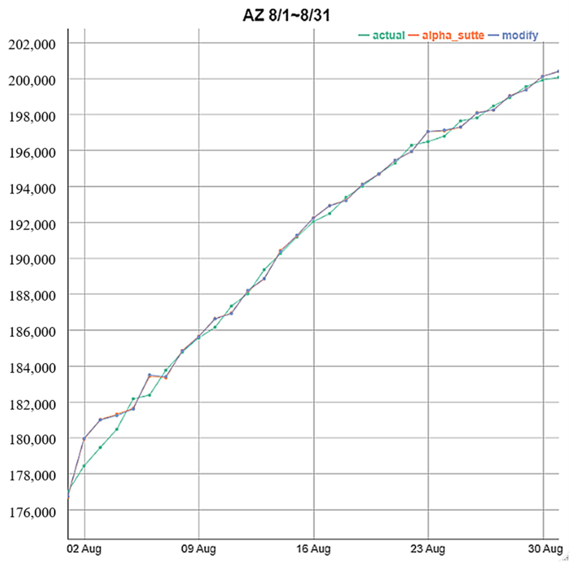
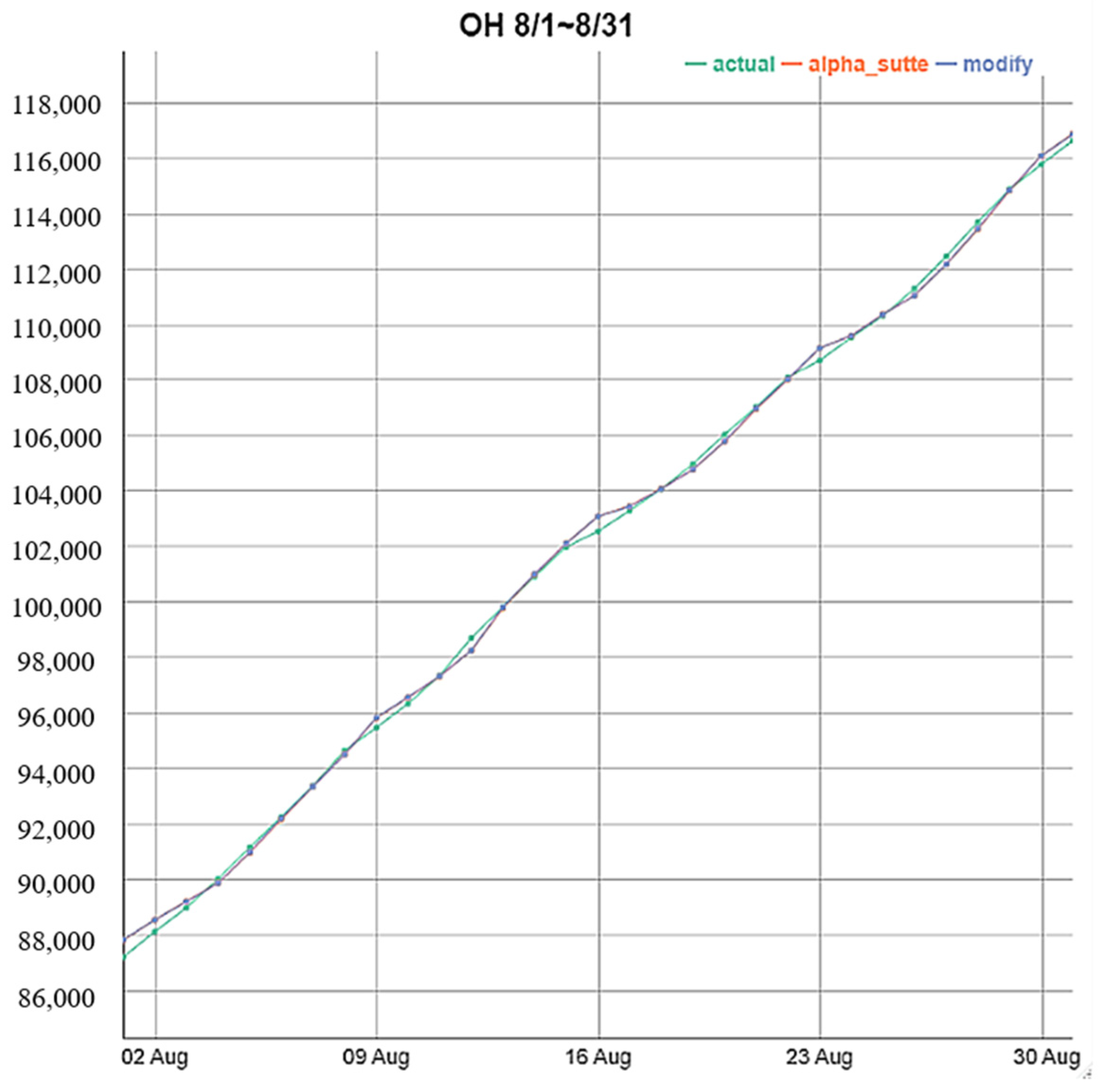
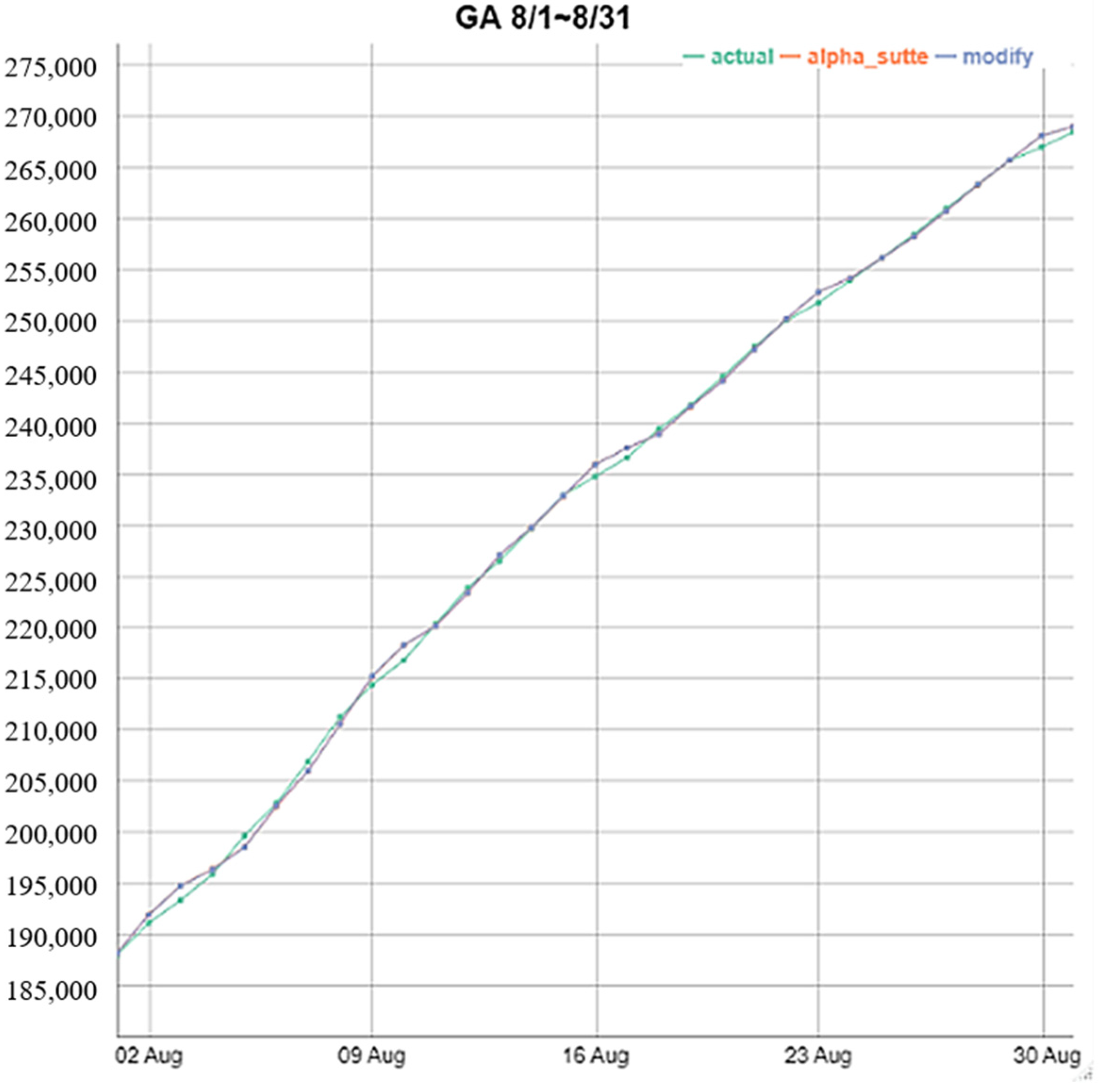
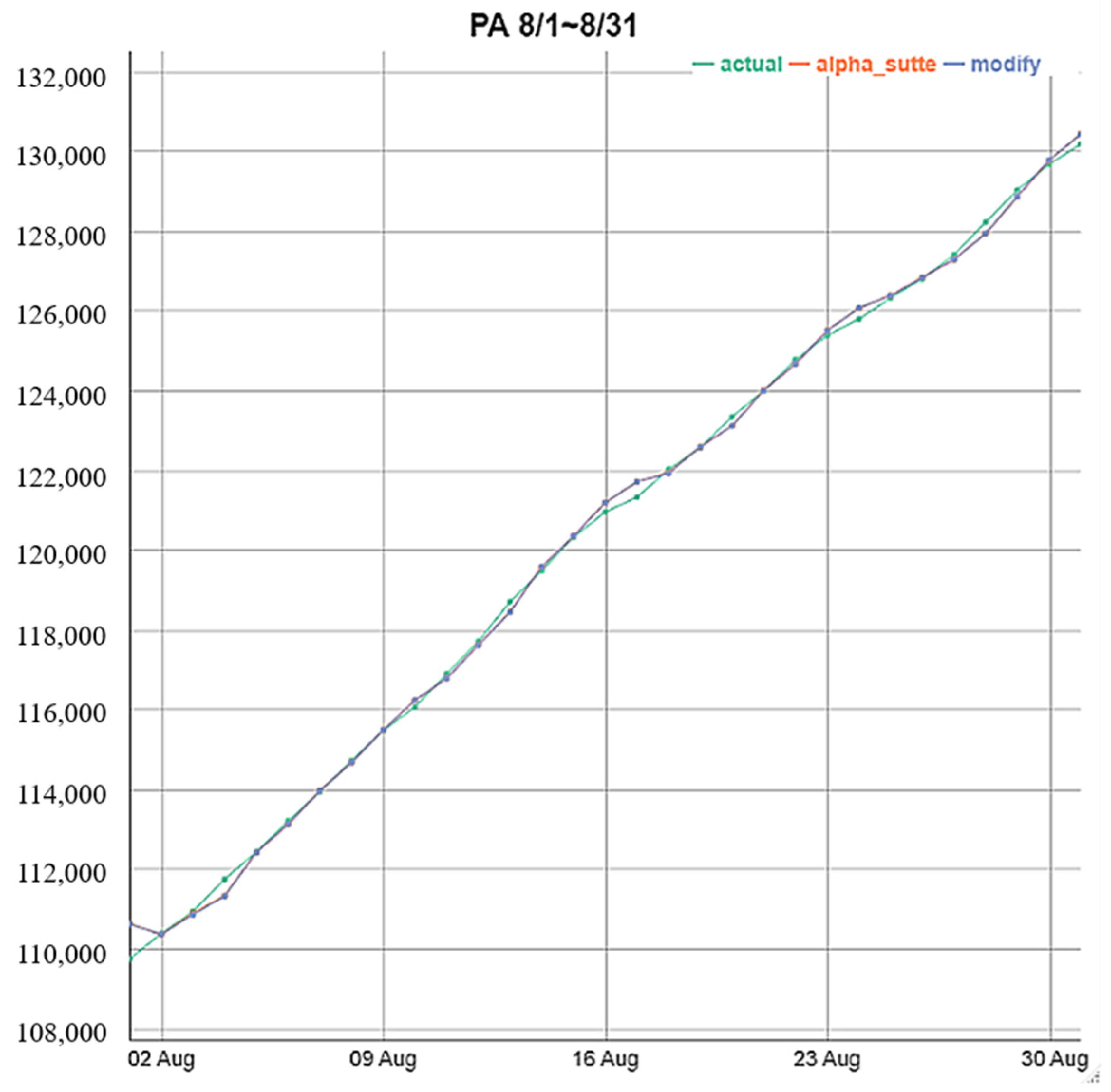
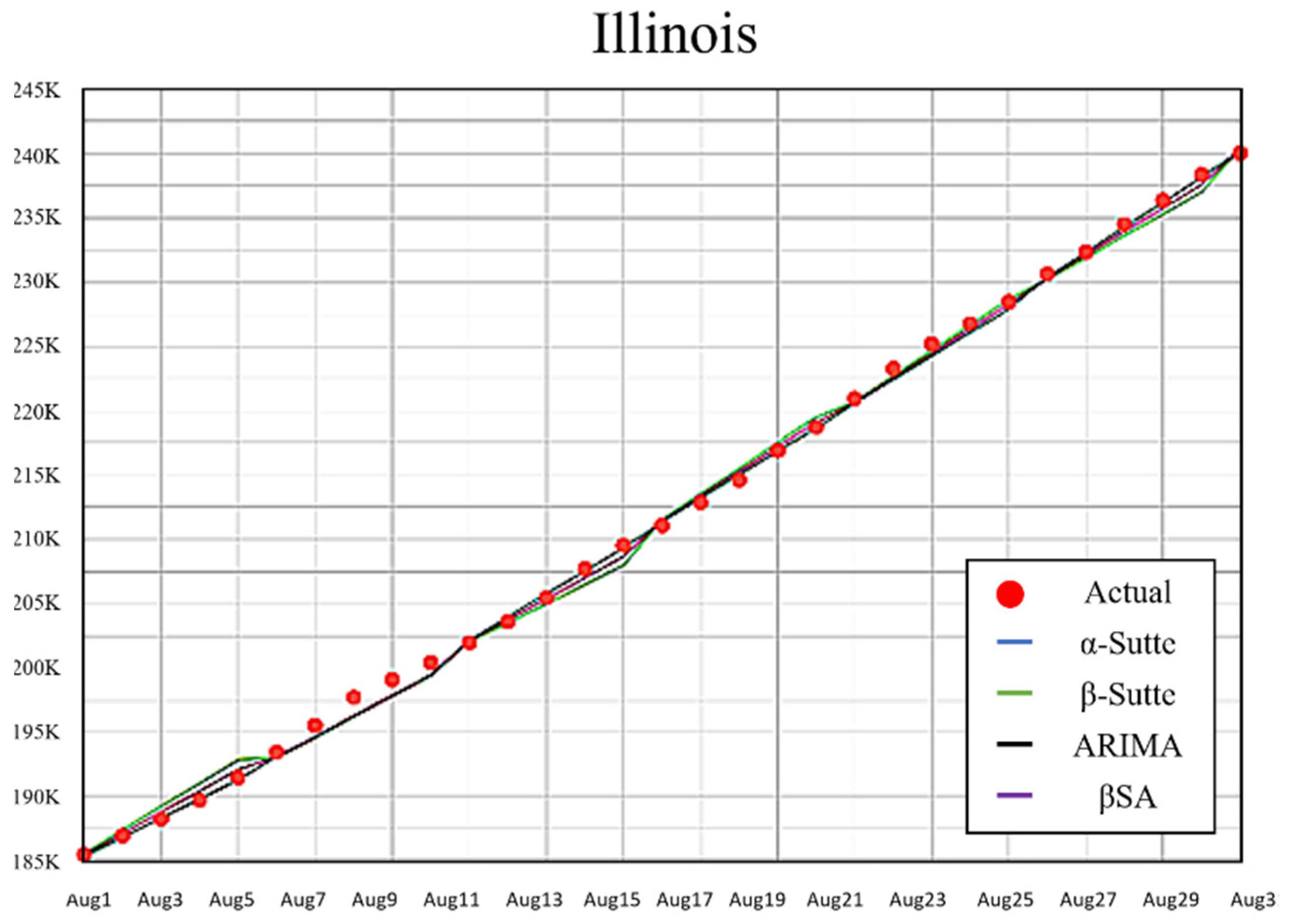
4.1. One-Day-Ahead Forecasting of the Cumulative Number of Confirmed Cases

One-day-ahead forecasting of the cumulative number of confirmed cases in the US are evaluated in this section. The five worst-hit states (IL, OH, GA, PA, AZ) in the cumulative number of confirmed cases are also included for comparison. Overall, four methods (α-Sutte indicator, β-Sutte indicator, ARIMA, and βSA) of forecasting are employed, each using a sliding window with 7-days training and one-day-ahead forecasting. The first training time period is 25 July 2020 to 31 July 2020, then, scrolls to the training interval step by step. The predicted testing time period is 1 August 2020 to 31 December 2020. The one-day-ahead forecasting results of the daily cumulative number of confirmed cases with metrics MAPE and RMSE are shown in

Table 3. Results of one-day-ahead forecasting (cumulative).

Area	Metrics	α-Sutte	β-Sutte	ARIMA	βSA
USA	MAPE	0.1394	0.1372	0.13273	0.13272
	RMSE	19644.57	19546.79	19614.3	19236.6
IL	MAPE	0.2273	0.2259	0.2205	0.2198
	RMSE	1616.399	1618.376	1636.707	1591.048
OH	MAPE	0.3085	0.3013	0.2921	0.2902
	RMSE	2127.701	2050.916	1989.027	2000.301
GA	MAPE	0.1830	0.1827	0.1746	0.1734
	RMSE	916.2098	914.0448	876.5051	877.3660
PA	MAPE	0.2191	0.2177	0.2232	0.2166
	RMSE	1041.438	1023.412	1005.699	994.5549
AZ	MAPE	0.2666	0.2699	0.2652	0.2603
	RMSE	1653.714	1662.204	1584.275	1607.716

. Since all the predicted values are close to the actual value, the US and five states (IL, OH, GA, PA, AZ) forecast trend only for August 2020 are demonstrated in Figure 2, Figure 3, Figure 4, Figure 5, Figure 6 and Figure 7.

4.2. Five Days Ahead Forecasting of the Cumulative Number of Confirmed Cases

Khan et al. [15] proposed that a flexible framework will help relevant departments formulate policies by predicting new infections of COVID-19 after 5 and 10 days. To observe the forecasting capability of our proposed β-Sutte indicator and βSA ensemble model further, the five days ahead prediction of the cumulative number of confirmed cases is also evaluated. Due to the fact that the actual data of five days ahead cannot be obtained in advance when forecasting, we assume that the dynamic weight in Equation (2) is fixed in the next four days’ forecasting except $\tilde{d}\left(t\right)$. Therefore, the other four days’ forecasting prediction is defined as Equation (5):

$$\tilde{d}\left(t+j\right)={\mathsf{\omega }}_a\left(t\right) · \tilde{a}\left(t+j\right)+{\mathsf{\omega }}_b\left(t\right) · \tilde{b}\left(t+j\right)+{\mathsf{\omega }}_g\left(t\right) · \tilde{g}\left(t+j\right)$$

(5)

where $\tilde{a}\left(t+j\right), \tilde{b}\left(t+j\right), \tilde{g}\left(t+j\right)$ are calculated from the previous forecasting value of $\tilde{d}\left(t+j-1\right), j=1, 2, 3, 4$.

Thus, five days ahead forecasting of the cumulative number of confirmed cases in the US and five worst-hit states (IL, OH, GA, PA, AZ) using four forecasting methods (α-Sutte indicator, β-Sutte indicator, ARIMA, and βSA) are evaluated. The data set and sliding window setting are the same as in Section 4.1. The evaluation results with metrics MAPE and RMSE of five days ahead are shown in

Table 4. Results of five days ahead forecasting (cumulative).

Area	Metrics	α-Sutte	β-Sutte	ARIMA	βSA
USA	MAPE	0.004448	0.004453	0.004195	0.004310
	RMSE	29848.19	29905.25	29127.87	29182.17
IL	MAPE	0.35	0.353	0.19	0.25
	RMSE	840.65	846.80	538.28	622.25
OH	MAPE	0.803	0.806	0.64	0.71
	RMSE	1067.16	1072.69	906.65	983.37
GA	MAPE	0.662	0.665	0.48	0.54
	RMSE	1974.65	1983.20	1523.24	1704.02
PA	MAPE	0.47	0.46	0.451	0.457
	RMSE	748.16	743.89	708.67	716.86
AZ	MAPE	0.60	0.61	0.81	0.70
	RMSE	1752.19	1786.45	2506.30	2125.71

. As an example, one monthly forecast trends of the US and Illinois State are shown in Figure 8 and Figure 9 for demonstration.

According to MAPE and RMSE in Table 4, it is found that the ARIMA method outperforms almost all other methods, and even outperforms our proposed βSA ensemble model for five day ahead predictions in all regions. A possible reason might be that fixed dynamic weights are assumed in the last four-day forecast, in Equation (2), which may need to be adjusted in a certain way rather than fixed. However, this question is left for other researchers to study further in the future.

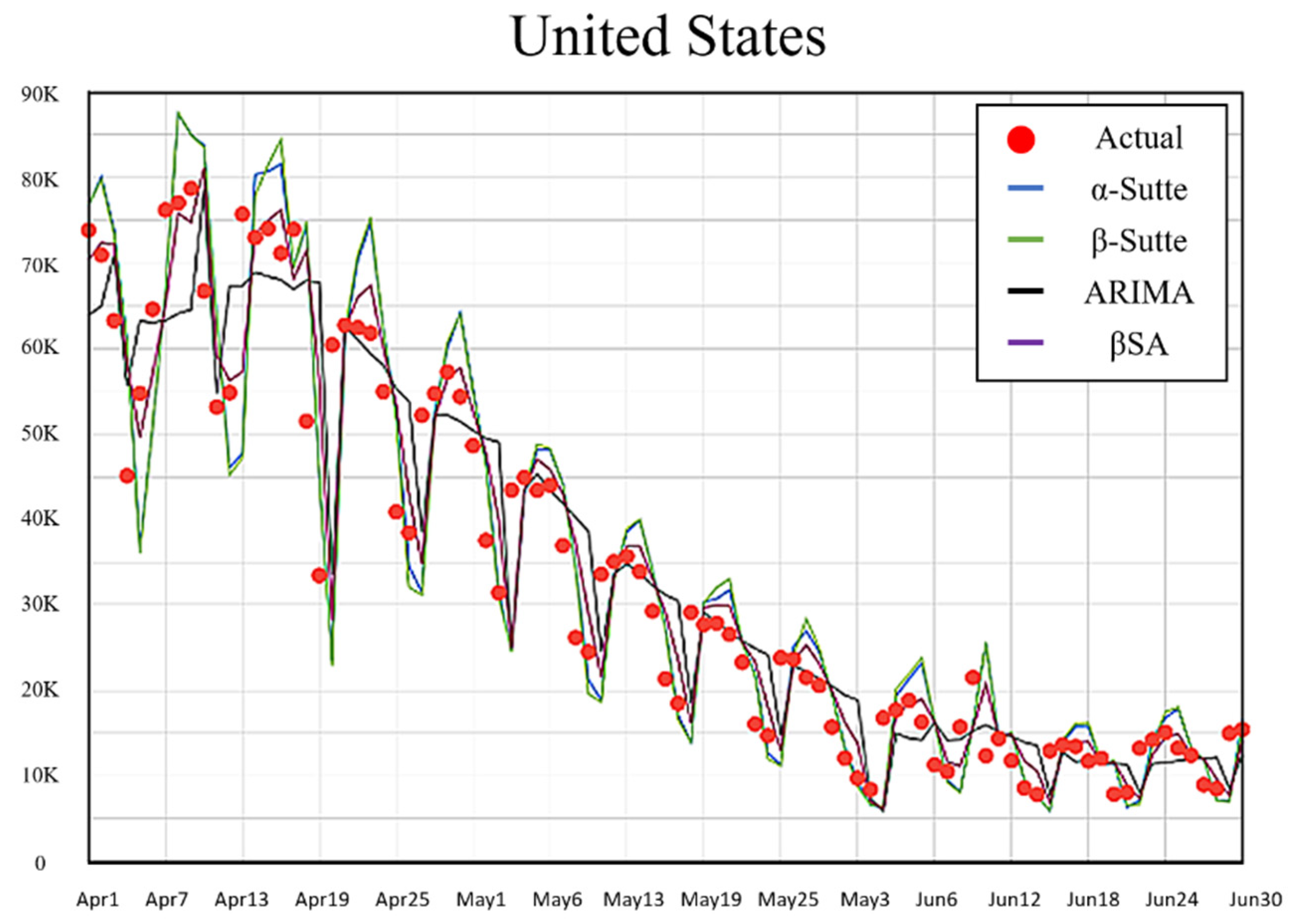
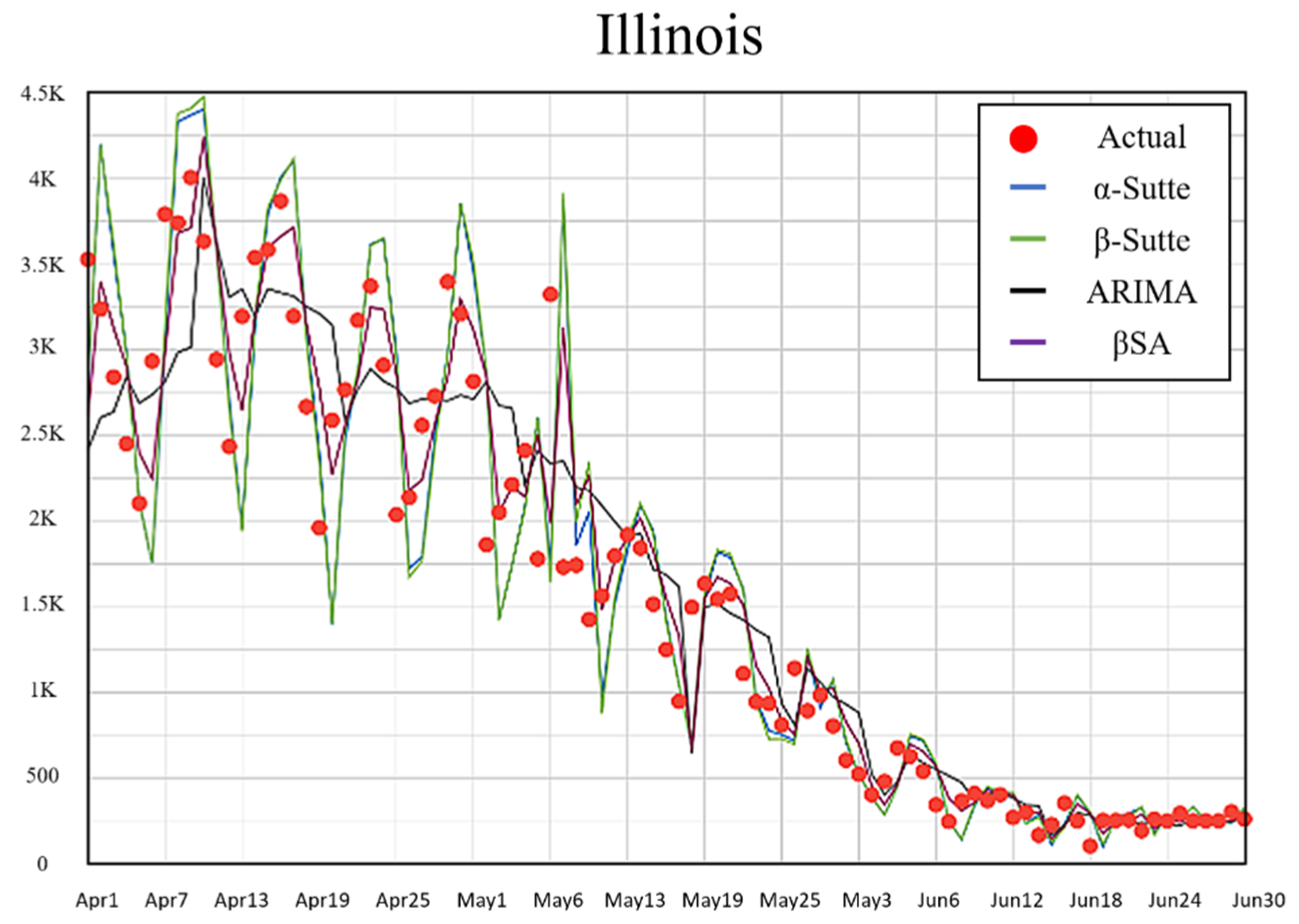
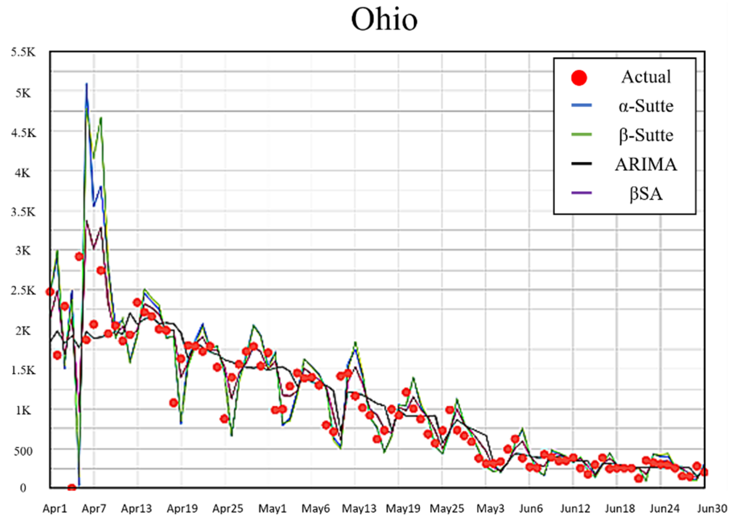
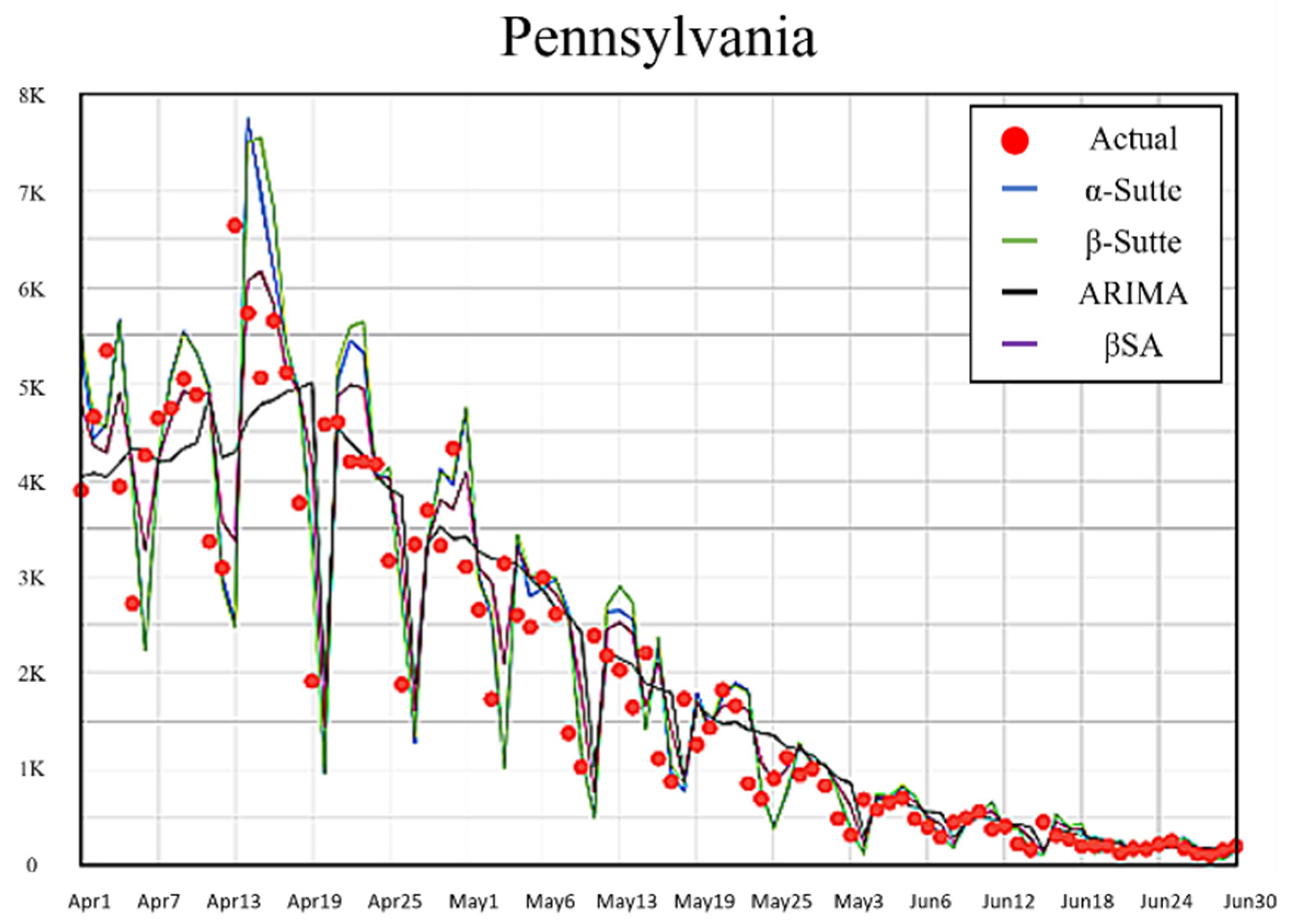
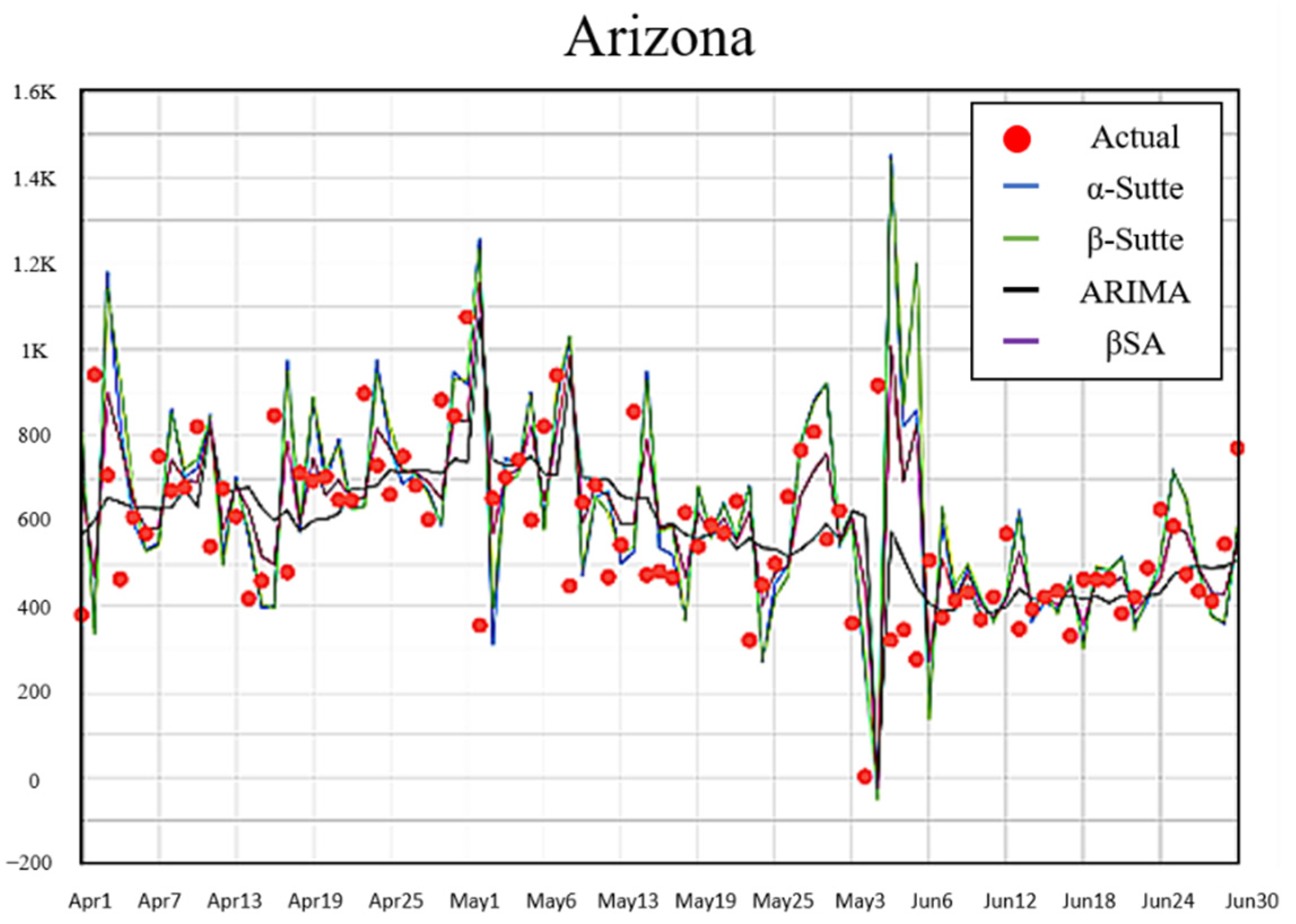
4.3. Forecasting of the Daily Number of Newly Confirmed Cases

Since the cumulative number of confirmed cases in the US are almost an incremental linear function, the capability of our proposed β-Sutte indicator and βSA ensemble model are tested by another vibration function, such as the daily number of newly confirmed cases.

Therefore, the daily number of newly confirmed cases in the US and five worst-hit states of confirmed cases are adopted, and four methods (α-Sutte indicator, β-Sutte indicator, ARIMA, and βSA) are used for testing their forecasting capability. The sliding windows setting is the same as in Section 4.1. As the United States invested in a large number of vaccines after July 2021, to avoid the interference of this event, the forecasting period time is set from 1 April 2021 to June 2021.

After calculation, Figure 10, Figure 11, Figure 12, Figure 13, Figure 14 and Figure 15 are the forecasting run charts of the number of newly confirmed cases daily by the four methods (α-Sutte indicator, β-Sutte indicator, ARIMA, and βSA) in each state, and the red dots stand for the actual values. The MAPE and RMSE of the daily number of newly confirmed cases using four forecasting methods are shown in

Table 5. Forecasting results of newly confirmed cases.

Area	Metrics	α-Sutte	β-Sutte	ARIMA	βSA
USA	MAPE	6754	6961	6222	5425
	RMSE	9311.46	9484.932	8647.039	7822.754
IL	MAPE	375	381	322	275
	RMSE	538.331	549.3422	442.886	404.925
OH	MAPE	350	369	219	254
	RMSE	648.322	666.000	357.165	441.814
GA	MAPE	236	242	202	191
	RMSE	333.009	338.687	275.697	262.301
PA	MAPE	618	643	496	514
	RMSE	980.757	1011.355	785.267	806.960
AZ	MAPE	197	202	132	154
	RMSE	287.056	297.131	198.661	231.292

. It can be seen from Table 5 that the MAPE and RMSE in the cases of the US, IL, and GA have the best forecasting accuracy of our proposed βSA ensemble model in this study. However, the ARIMA method takes the lead in the cases of OH, PA, and AZ. It can be said that these two methods, ARIMA and the proposed βSA ensemble, are comparable in forecasting performance.

5. Conclusions

This study proposes a novel β-Sutte indicator and βSA ensemble model modified from the α-Sutte indicator [16] for forecasting. To evaluate the performance of our proposed β-Sutte indicator, four methods (α-Sutte indicator, β-Sutte indicator, ARIMA, and βSA) are compared through the forecasting of confirmed COVID-19 cases in cumulative one-day-ahead, cumulative five days ahead, and the daily number of newly confirmed cases on the five worst-hit states in the US.

Experimental results show that our proposed β-Sutte indicator using dynamic weighting has a better performance than the original α-Sutte indicator in general. However, for more complex calculations, the ARIMA model can overcome the performance of α-Sutte indicator and β-Sutte indicator. Nevertheless, our proposed βSA ensemble model is among the best in these four forecasting methods generally.

Recommendations for future research are:

• The dynamic weight of the β-Sutte indicator proposed in this study needs seven days of in training advance, thus the time cost will be higher than the four days preset by the α-Sutte indicator. Moreover, the ARIMA model needs even more time cost for training. Therefore, how to decide which one is the best to use is an issue.
• The β-Sutte indicator proposed uses an error-based weighting method to improve the original α-Sutte indicator. In the future, perhaps other weighting methods can be used to increase the performance, such as entropy weighting, genetic algorithm, etc.
• The βSA ensemble model proposed in this study adopts a mean distributed weight method. In the future, perhaps different weighted distribution methods can be used for ensemble weight adjustment.
• Due to the many external variables involved with confirmed COVID-19 cases, other variables could be considered in the future (for example: death rate, transmission rate, etc.), and, combined with other deep learning methods, machine learning methods as a hybrid or ensemble model also have a chance to further improve the accuracy of forecasting.

References

1. Zhang, X.; Ma, R.; Wang, L. Predicting turning point, duration and attack rate of COVID-19 outbreaks in major Western countries. Chaos Solitons Fractals 2020, 135, 109829. [Google Scholar] [CrossRef] [PubMed]
2. Alazab, M.; Awajan, A.; Mesleh, A.; Abraham, A.; Jatana, V.; Alhyari, S. Covid-19 prediction and detection using deep learning. Int. J. Comput. Inf. Syst. Ind. Manag. Appl. 2020, 12, 168–181. [Google Scholar]
3. Chimmula, V.K.R.; Zhang, L. Time series forecasting of COVID-19 transmission in Canada using LSTM networks. Chaos Solitons Fractals 2020, 135, 109864. [Google Scholar] [CrossRef] [PubMed]
4. Utkucan, Ş.; Tezcan, Ş. Forecasting the cumulative number of confirmed cases of COVID-19 in Italy, UK and USA using fractional nonlinear grey Bernoulli model. Chaos Solitons Fractals 2020, 138, 109948. [Google Scholar] [CrossRef]
5. Williamson, E.J.; Walker, A.J.; Bhaskaran, K.; Bacon, S.; Bates, C.; Morton, C.E.; Inglesby, P. Factors associated with COVID-19-related death using OpenSAFELY. Nature 2020, 584, 430–436. [Google Scholar] [CrossRef] [PubMed]
6. Zhou, F.; Yu, T.; Du, R.; Fan, G.; Liu, Y.; Liu, Z.; Xiang, J.; Wang, Y.; Song, B.; Gu, X.; et al. Clinical course and risk factors for mortality of adult inpatients with COVID-19 in Wuhan, China: A retrospective cohort study. Lancet 2020, 395, 1054–1062, Erratum in Lancet 2020, 395, 1038. [Google Scholar] [CrossRef]
7. Mehdiyev, N.; Enke, D.; Fettke, P.; Loos, P. Evaluating forecasting methods by considering different accuracy measures. Procedia Comput. Sci. 2016, 95, 264–271. [Google Scholar] [CrossRef] [Green Version]
8. Ahmar, A.S.; Rahman, A.; Mulbar, U. Implementation of α-Sutte Indicator to Forecasting Consumer Price Index in Turkey. In Proceedings of the International Conference On Mathematics and Natural Sciences, Bali, Indonesia, 6–7 September 2017; pp. 1–4. [Google Scholar] [CrossRef]
9. Al-Dahidi, S.; Baraldi, P.; Zio, E.; Legnani, E. A dynamic weighting ensemble approach for wind energy production prediction. In Proceedings of the 2017 2nd International Conference on System Reliability and Safety (ICSRS), Milan, Italy, 20–22 December 2017. [Google Scholar]
10. Abdollahi, H.; Ebrahimi, S.B. A new hybrid model for forecasting Brent crude oil price. Energy 2020, 200, 117520. [Google Scholar] [CrossRef]
11. Abolmaali, S.; Shirzaei, S. A comparative study of SIR Model, Linear Regression, Logistic Function and ARIMA Model for forecasting COVID-19 cases. AIMS Public Health 2021, 8, 598–613. [Google Scholar] [CrossRef] [PubMed]
12. Ahmar, A.S.; Del Val, E.B. SutteARIMA: Short-term forecasting method, a case: Covid-19 and stock market in Spain. Sci. Total Environ. 2020, 729, 138883. [Google Scholar] [CrossRef] [PubMed]
13. Kim, S.; Kim, H. A new metric of absolute percentage error for intermittent demand forecasts. Int. J. Forecast. 2016, 32, 669–679. [Google Scholar] [CrossRef]
14. Chicco, D.; Warrens, M.J.; Jurman, G. The coefficient of determination R-squared is more informative than SMAPE, MAE, MAPE, MSE and RMSE in regression analysis evaluation. PeerJ. Comput. Sci. 2021, 7, e623. [Google Scholar] [CrossRef]
15. Khan, F.; Ali, S.; Saeed, A.; Kumar, R.; Khan, A.W. Forecasting daily new infections, deaths and recovery cases due to COVID-19 in Pakistan by using Bayesian Dynamic Linear Models. PLoS ONE 2021, 16, e0253367. [Google Scholar] [CrossRef]
16. Ahmar, A.S. α-Sutte Indicator: Suatu Pendekan Baru dalam Peramalan Data. Monograph 2017, 1–5. [Google Scholar] [CrossRef]
Figure 1. Flow chart of the experiment.
Mathematics 10 00824 g001
Figure 2. United States forecast trend (one day).
Mathematics 10 00824 g002
Figure 3. Illinois State’s forecast trend (one day).
Mathematics 10 00824 g003
Figure 4. Ohio State’s forecast trend (one day).
Mathematics 10 00824 g004
Figure 5. Georgia State’s forecast trend (one day).
Mathematics 10 00824 g005
Figure 6. Pennsylvania State’s forecast trend (one day).
Mathematics 10 00824 g006
Figure 7. Arizona State’s forecast trend (one day).
Mathematics 10 00824 g007
Figure 8. United States forecast trend (five days).
Mathematics 10 00824 g008
Figure 9. Illinois State’s forecast trend (five days).
Mathematics 10 00824 g009
Figure 10. United States forecast trend (new cases).
Mathematics 10 00824 g010
Figure 11. Illinois State’s forecast trend (new cases).
Mathematics 10 00824 g011
Figure 12. Ohio State’s forecast trend (new cases).
Mathematics 10 00824 g012
Figure 13. Georgia State’s forecast trend (new cases).
Mathematics 10 00824 g013
Figure 14. Pennsylvania State’s forecast trend (new cases).
Mathematics 10 00824 g014
Figure 15. Arizona State’s forecast trend (new cases).
Mathematics 10 00824 g015