Decomposition of the Knapsack Problem for Increasing the Capacity of Operating Rooms ^†

Abstract

This paper is aimed at the problem of scheduling surgeries in operating rooms. To solve this problem, we suggest using some variation of the bin packing problem. The model is based on the actual operation of 10 operating rooms, each of which belongs to a specific department of the hospital. Departments are unevenly loaded, so operations can be moved to operating rooms in other departments. The main goal is to increase patient throughput. It is also necessary to measure how many operations take place in other departments with the proposed solution. The preferred solution is a solution with fewer such operations, all other things being equal. Due to the fact that the mixed-integer linear programming model turned out to be computationally complex, two approximation algorithms were also proposed. They are based on decomposition. The complexity of the proposed algorithms is estimated, and arguments are made regarding their accuracy from a theoretical point of view. To assess the practical accuracy of the algorithms, the Gurobi solver is used. Experiments were conducted on real historical data on surgeries obtained from the Burdenko Neurosurgical Center. Two decomposition algorithms were constructed and a comparative analysis was performed for 10 operating rooms based on real data.

1. Introduction

Health scheduling is an essential component for medicine automation. The development of scheduling models and algorithms has gained particular relevance in connection with the COVID-19 pandemic. In particular, there is a high demand for scheduling operating rooms. In Russia, many operations can be done free of charge according to a government quota. If the operation is considered urgent, the patient might agree to a paid service and later apply for compensation. Each surgical department has its own peculiarities of functioning. This is the time and principles of the work of anesthesiologists, the possibility of performing operations in other departments and associated overlays, the scheduling and rotation of doctors, and much more. For a multidisciplinary surgical hospital, an unbalanced operation of the surgical department is a limiting factor for the overall functioning of the organization. This is especially important for neurosurgical clinics, where individual surgical rooms are specialized and equipped to carry out certain types of surgery.

Due to modern technology, medical care is becoming automated. Therefore, the study of optimizing service processes is relevant. There are many publications on health scheduling. Let us consider some papers for the investigated problem of optimizing surgery rooms. The papers [1,2] are dedicated to an analysis of OR (operating room) and surgery scheduling. They highlight three decision levels in OR scheduling and planning: strategic, tactical, and operational. The strategic level covers long-term decisions, such as capacity planning and allocation, which typically take a long time. In such problems, the amount of time a given OR is dedicated to a surgical specialty is determined in order to optimize profit/cost over a long period. Problems with cyclic OR schedules, such as master surgical scheduling, are categorized at the tactical level. Moreover, the last decision level, the operational level, is the shortest and involves decisions such as resource allocation, surgical cases, and advanced scheduling. Our problem belongs to the operational level, our main goal is to distribute elective surgeries in operating rooms. There are also three well-known scheduling strategies/booking systems that dedicate OR-time to surgical groups: open scheduling strategy, block scheduling strategy, and modified block scheduling strategy. In reference [3], the authors used the block scheduling strategy, and tried to maximize the occupation of the ORs and respect the order of patients in the waiting list as much as possible. They used normal distribution for the duration of surgeries and cleaning time. In an objective function, the authors identified three criteria. The first is to maximize the expected surgery time in each block. The second criteria sets the probability that the total work duration of each time block does not exceed the available time. Furthermore, the last criteria ensures that preference is given to the first patients in the waiting list. However, they do not take into account differences between operating rooms. We also put patients from the waiting list to ORs using a block scheduling strategy but in our model different ORs belong to different departments, and we have to take this into account. Paper [4] shows the operating room scheduling problem, such as the bin packing problem. The authors look for a schedule with all n activities programmed to run in a container such that the container capacity is not exceeded and the downtime is minimal. Since the number of possible schedules grows exponentially, the complexity of solving these problems is due to the number of combinations that a large set of activities generate. This fact often leads to delays in the scheduling process, as the ease of finding an efficient schedule is reduced. To solve the problem, they developed a genetic algorithm. Genes are used to model time spaces in which jobs can be scheduled. Each gene has a length that cannot be exceeded. A chromosome contains a group of genes. In other words, each chromosome represents a possible schedule of work. In this representation, chromosomes may vary in size depending on the number of operating rooms used in the solution. We decided to use the bin packing problem with a homogeneous capacity in our model. The authors of paper [5] compare batched and online scheduling in surgery scheduling; in our model we use batched scheduling, the waiting list is updated every week, and patients are scheduled for the following week. The policy in batch schedules works as follows: it ignores new arrivals when the schedule is over. Thus, this class only cares about the result within the time horizon. Optimal solution methods for such schedules may include mixed-integer linear programming (MILPs) solvers. These can be optimal solvers based on branching and cutting methods or metaheuristics. Batch scheduling works as follows: when a certain number of people in a batch is recruited, a schedule is made for the current day. People who have already been enrolled are removed from the upcoming batch, and new patients and those not yet enrolled are put into the next batch scheduling for the next day. Batch scheduling problems are often simpler, but can involve many different constraints. Paper [6] solves a problem close to ours. In that paper, the authors present an optimization framework for batch scheduling within a block-booking system that maximizes the expected utilization of operating room resources subject to a set of probabilistic capacity constraints. To understand whether a given schedule is feasible or not, the scheduler uses an estimate provided by the surgeon and an estimate based on historical data. If the sum of the point estimates of the duration of the operations assigned to the same schedule block and the intermediate cleaning time does not exceed the block length, then the block assignment is considered feasible. Note that we use historical data of a hospital too. The main purpose of this strategy is to ensure that all scheduled surgeries can be finished within the allotted block length, avoiding overtime. They solved the problem with mixed-integer programming and we also use this method. The authors develop an algorithm based on a normal approximation for the sum of the surgery duration to provide near-optimal solutions to the stochastic scheduling problem. The primary aim of paper [7] is the effective and balanced use of equipment and resources in hospital operating rooms. In this context, datasets from a state hospital were used via the goal programming and constraint programming methods. Now, we consider more contemporary papers in surgery scheduling. In research [8] from 2021, the authors use a weekly surgery schedule with an open scheduling strategy. In our work, we also construct a weekly schedule. The objective is to minimize the total operating cost while maximizing the utilization of the operating rooms, while also minimizing overtime use. Their mathematical model can provide optimal solutions for a surgery size of up to 110 surgical cases. Furthermore, the authors proposed two modified heuristics, based on the earliest due date and longest processing time rules, to quickly find feasible solutions. In article [9] from 2021, the authors find the optimal schedule of surgeries by minimizing operating rooms’ idle times (in our paper we minimizing idle times too) while maximizing the number of scheduled surgeries during the most effective and desirable time windows. Surgeries during ideal time windows are encouraged by assigning bonus weights in the objective function. The stated and implied benefits of this strategy include mitigating financial loss, complications, and death rate due to a reduction in surgery delays. They introduce a binary programming model for scheduling operating rooms and a mixed-integer binary program for planning and scheduling both operating and recovery rooms for elected patients under deterministic conditions. The authors apply an open scheduling strategy for assigning operating rooms to surgeons and a Lagrangian relaxation method for finding promising solutions. Consider another article, namely [10] from 2021, which is similar to ours. In this paper, the authors allocate elective patients and resources (i.e., operating rooms, surgeons, and anesthetists) to days, assign resources to patients, and sequence patients in each day. They consider patients’ due dates, resource eligibility, the heterogeneous performances of resources, downstream unit requirements, and lag times between resources. The goal is to create a weekly surgery schedule that minimizes fixed and overtime costs. To efficiently and effectively solve the problems of MILP models, the authors develop new multi-featured logic-based Benders decomposition approaches. Furthermore, a lot of works, such as [11,12,13], have an uncertain duration of surgery, and we plan to include this complication. In this paper, we do not consider the uncertainty. Our work is organized as follows: We consider the mathematical model in Section 2. Section 3 reviews the computational experiments. The decomposition algorithms are shown in Section 4. Section 5 presents the results of the algorithms compared to the MILP. Furthermore, some remarks are presented in the Conclusion section.

2. Mathematical Model

2.1. Problematic

The goal is to increase throughput according to two factors: reducing gaps in schedules and increasing the operation time in ORs. We can use the information system of the Burdenko Neurosurgical Center and doctors’ expert evaluations to solve the problem. Experts identify subproblems such as hospitalization, surgical department manipulations, and the monitoring of surgery rooms. The problem is divided into three subproblems: The first is the problem of allocating specialists to the appropriate rooms at a certain time. The second problem is to create a schedule for receiving patients for surgery. The third one is the problem of predicting the idle times of surgery rooms.

In this paper, we consider only assignment patients to ORs. There are 10 departments in the Burdenko Neurosurgical Center, and each department has its own operating room. Incoming patients are always assigned to one of these departments. We will consider only elective patients. The Burdenko Neurosurgical Center information system includes information about a patient’s hospitalization, the principles of their treatment, and the work of the department, including occupied beds and the work of the surgical department, etc. For each patient, information about their operations is generated in the system. This creates a table that consists of the following columns: number of the patient; date; the host department; surgery room ID; complexity category of surgery; start of surgery; end of surgery. Based on this table, we can conclude that the usage periods of ORs usually have gaps, which greatly reduces the efficiency of ORs. According to examples for each surgery, we know the duration, number, and the department in which it should be performed. By using these examples, we created the frequency dictionary of various parameters and used it in the generation. Each department has its operating room. However, we can try to allocate some operations of the busy departments to the operating rooms of less busy departments.

2.2. Model

Let $M=1,2,...,m$–set of operating rooms, $O=1,2,...,o$–set of departments, and $J=1,2,...,n$–set of surgeries. We consider 10 operating rooms $m_i\in M$ that work 4 days a week for 11 h every day (from 9:00 to 20:00). Our main goal is to decrease the gaps in these operating rooms. Gaps there mean that the operating room is not busy at these moments. Analyzing the hospital report, we can see that the duration of surgeries is quite long. Let us assume that if the surgery ends at 17:00, then there will be no others after it because there is a high risk of overtime work. Because of this, there are gaps in the schedule. To solve this problem, we suggest using some variation of the bin packing problem, as containers will be operating rooms, the capacity of which is determined by the number of hours during which the surgeries can be performed (11 h). This model does not include urgent patients. We receive a patient waiting list at the end of each week and make a schedule for the next working week. In this case, the schedule is not a specific time for the start of operations, but only the distribution of surgeries in the ORs and days. The main goal is to decrease the number of gaps in the OR’s schedule for the whole working week. Furthermore, an important criterion is a department where the patient is treated, because each department $o_i\in O$ has its own OR $m_i$ (10 departments), and it is undesirable to operate the patient in an external OR. In our previous work on this topic [14], we approached this problem in terms of schedule theory, and we assigned patients strictly to their operating rooms. However, in this work, for this purpose, a weight matrix W has been added to the model, where $w_{ij}=w_0$ ($w_0>1$), if the surgery j is performed in “its” OR $m_i$, and $w_{ij}=1$ in the other case. The definition of a guest surgery and a home surgery is introduced; we will call the surgery “home” if it is performed in “its” operating room, and we will call the surgery “guest” if it is performed in another operating room. Let us construct a mathematical model. The parameters of the model are:

• $p_j$—processing time of surgery j, $\forall j\in J$;
• $w_{ij}$—weight of surgery j, if it is being performed in OR i, $\forall i\in M$;
• D—set of days when you can perform the surgery. In our case it is $d=1,2,3,4$ (Monday, Tuesday, Wednesday, Thursday);
• A—operating room hours per day (11 h).

The variables of the model are:

• $x_{ij}^d=1$, iff surgery j assigned to OR i on day d, and equal 0 otherwise.

Objective function:

$$\sum _{d\in D}\sum _{i\in M}\sum _{j\in J}{x}_{ij}^d{p}_j{w}_{ij}\to max$$

(1)

Subject to:

$$\sum _{d\in D}\sum _{i\in M}{x}_{ij}^d\le 1,\forall j\in J;$$

(2)

$$\sum _{j\in J}{p}_j{x}_{ij}^d\le A,\forall i\in M,\forall d\in D.$$

(3)

The objective function (1) maximizes the weighted number of operating hours during the week, which, accordingly, minimizes gap hours. Constraint (2) ensures that one operation is not scheduled more than once. Furthermore, constraint (3) guarantees that the total duration of all surgeries in one OR on one day does not exceed the operating time of that room; in our case all operating rooms work the same number of hours. It is also necessary to note that this problem is NP-hard and cannot be solved in polynomial time.

3. Computational Experiments

Experiments will be conducted on pseudo-real data. Surgical data were provided to us by Burdenko Neurosurgical Center. The Burdenko National Medical Research Center for Neurosurgery is the leading neurosurgical hospital in the Russian Federation and the world’s leading neurosurgical clinic, with a rich history, state-of-the-art equipment, and a unique professional team. Every year the National Center performs about 10,000 neurosurgical surgeries for the widest range of diseases of the nervous system. The structure of the center includes 10 clinical departments with 10 main operating rooms. We have data on all surgery operations made in 2014. It is also important to note that some operating rooms are busier than others. In other words, operations are assigned to operating rooms unevenly. The duration of surgical operations is generated randomly, with a variation of one hour from the average duration of surgeries in a given department. Thus, our dataset contains the department to which the surgery is attached and the duration of this surgery. The MILP model in all experiments is solved using Gurobi with an academic license in a Python environment. We decided to use Gurobi since it is the most powerful mathematical optimization solver.

The simulation scheme is as follows:

• At the beginning of the week, N of generated surgeries is added to the waiting list;
• The problem of mixed-integer linear programming with the above-described constraints and objective functions is solved by Gurobi in Python. That is, the optimal schedule for a given week is made, and the surgeries that could not be assigned remain in the waiting list and are transferred to the next week;
• Furthermore, this cycle is repeated.

The number of surgeries N that we add to the waiting list every week is important. On average, about 130–140 surgeries are performed per week. Accordingly, if we take N much more than this value, the operations will accumulate in the waiting list, and with each week the gaps will become smaller because there will be a large selection of surgeries to schedule. However, the queue will keep steadily growing.

We need to minimize the total gap hours concerning the fact that guest surgeries are undesirable. Then, we need to check the dependency of OR’s gap hours, and the number of guest surgeries, depending on the choice of weight $w_0$. The planning period is chosen to be two weeks and the number of surgeries $N=150$, so that a large number of surgeries would not accumulate. We tested the experiments on five different generated data, where only the duration of surgeries changes randomly. We took the average values of the total gap duration and the number of guest surgeries for each experiment.

Figure 1 shows a sharp jump at the beginning. In Figure 2 with the increased scale, you can see that the jump occurs when the weight coefficients $w_0$ are from 1 to 4. Next, with the further increasing of weights, the value of the total gaps stabilizes at approximately 11 h.

Now, let us consider the graph of dependence of the number of guest surgeries on the same $w_0$ weighting coefficients (Figure 3 and Figure 4). This graph behaves almost in the same way; there is a sharp jump down with small values of $w_0$. Next, with the further increasing of weights, the number of the guest surgeries becomes stable, starting with the same values of $w_0$ as in the previous graph. The following conclusion can be drawn from these graphs: Even if it is very important to perform home surgeries ($w_0\gg 1$), we need to assign some guest surgeries (Figure 4) to make an optimal schedule. Furthermore, it appeared that the total duration of gaps also does not change at large values of $w_0$. The problem appeared to be computationally difficult for weights, at which there is a sharp jump in the graphics. That is the reason for adding a time limit to the experiment. If for a certain weight $w_0$ it takes a long time to calculate the result, then we skip this value and proceed with the next value of weight.

4. Algorithms

Since our MILP model is computationally difficult, we consider two approximate algorithms and compare them with each other. First, the algorithm constructs a schedule for each department separately, and after that, it changes some surgeries to more optimal solutions. In the second algorithm, we construct a decomposition graph to divide departments into groups and solve the MILP problem for each group.

4.1. Vertex Decomposition with Balanced Distribution

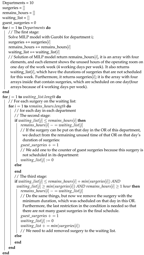
Vertex decomposition with balanced distribution further in the text will be called Algorithm 1. The main idea of this algorithm is to assign patients to ORs in their departments at first. This is the first stage. After this distribution, we have a schedule without guest surgeries and some patients remained on the waiting list. Next, at the second stage, we check if the patients from the waiting list can be assigned to any OR on any day of the week. Next, at the third stage, our algorithm checks if it is possible to assign patients from the waiting list to the OR if the surgery with the minimum duration is removed from it. Removed surgeries are added back to the waiting list and all steps of the algorithm are repeated for these surgeries. The third stage of the algorithm may be repeated several times. We look at the maximum value of the following values for all operation rooms and for all days: the remaining hours in the operating room if we remove the surgery with the minimum duration. Furthermore, this value is compared to the duration of the minimal surgeries on the waiting list; if it is more than the duration of two or one surgeries, we repeat the third stage twice or once, respectively. In our case, we always get one repetition of the third stage. As a reminder, our main goal is to minimize gaps in all ORs during the week. At first, we need to set a problem for the first step, whereby we construct a schedule without guest surgeries. It is a MILP model with the following parameters, objective functions, and constraints:

• $p_j$—processing time of surgery j, $\forall j\in J$;
• D—set of days when you can perform the surgery. In our case it is $d=1,2,3,4$ (Monday, Tuesday, Wednesday, Thursday);
• A—operating room hours per day (11 h).

The variables of the model are:

• $x_j^d=1$, iff surgery j assigned to OR on day d, and equal 0 otherwise.

Objective function:

$$\sum _{d\in D}\sum _{j\in J}{x}_j^d{p}_j\to max$$

(4)

Subject to:

$$\sum _{d\in D}{x}_j^d\le 1,\forall j\in J;$$

(5)

$$\sum _{j\in J}{p}_j{x}_j^d\le A,\forall d\in D.$$

(6)

The solution of this MILP model presents an optimal weekly schedule for one department if there are no guest surgeries. We solve this problem 10 times for each department (for each OR) and put all unassigned patients in the general waiting list. For a better understanding, we present the pseudocode of our Algorithm 1.

In our first experiment, we constructed a schedule for two weeks. Now we need to construct a schedule for two weeks for this algorithm. To achieve this, it is necessary to use the algorithm twice, but the second time the waiting list will not be empty, it will remain from the previous week. Furthermore, we can construct a schedule for N weeks, we just need to perform this algorithm N times and add unscheduled surgeries from previous weeks to the waiting list.

Algorithm 1: pseudocode

Remark 1.

At the third stage, we have restriction $remains\_hours\left[i\right]>T$, which means that we consider only ORs with more than T hours left for surgeries. Here, we took $T=1$ h, but in future works, we will find the cost of an operational hour and the cost of one guest surgery, and then calculate T based on these considerations, because T affects gap hours and the number of guest surgeries.

4.2. Graph Decomposition

Graph decomposition further in the text will be called Algorithm 2. Furthermore, we consider another approach to solve this problem. It is based on the mathematical model (1)–(3) (our exact approach); however, there, we break down the departments into groups. In other words, we solve several of the same problems with a smaller set of variables instead of one big problem with 10 departments. We can use the historical data of surgeries of each department and see which departments are overloaded and which are not, and combine them into groups. It can be represented with a graph (Figure 5): vertexes are the departments, one department can operate on patients from another department if there is an edge between them. We also solve this problem for N times to do the schedule for N weeks. In our case $N=2$.

So we need to solve our MILP model for every component of this graph. Now, we can compare three approaches on the same generated data in terms of the number of guest operations, the amount of unused work time in two weeks, and computing time. Below is the pseudocode of this algorithm.

Algorithm 2: pseudocode

4.3. Complexity of the Algorithms

In general, the upper bound of the efficiency of our MILP problem using the exact approach is brute force: $2^n$. In our case, n is equal to the number of binary variables $x_{ij}^d$, $n=N·M·D$, where N—the number of the surgeries, M—the number of the operation rooms, and D—the number of workdays in a week. Let the efficiency estimate of the algorithm for solving a discrete optimization problem with n binary variables be:

$$\varphi \left(n\right)=2^n.$$

(7)

Furthermore, let there be a tree that divides the problem into r blocks. It is argued that when decomposing the problem into blocks, the efficiency estimate of the entire problem will be equal to:

$$\sum _{i\in r}\varphi \left(n_i\right)=\sum _{i\in r}{2}^{n_i},$$

(8)

where $n=n_1+n_2+...+n_r$.

Property 1.

The estimate (8) is better than (7).

Proof. 

Using the well-known inequality $2^{x+y}>2^x+2^y$, $x,y>1$ we can write the following chain of inequalities:

$$2^{n_1+n_2+...+n_r}>2^{n_1}+2^{n_2+...+n_r}>...>2^{n_1}+2^{n_2}+...+2^{n_r}.$$

(9)

As a result, we observe that the decomposition increases the efficiency of the algorithm. □

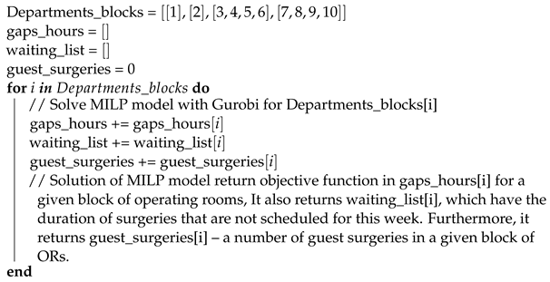
In Algorithm 2, we decompose our problem into four subproblems: $n=n_1+n_2+n_3+n_4$. Furthermore, the MILP problem becomes much easier, because the efficiency estimate now is equal to $2^{n_1}+2^{n_2}+2^{n_3}+2^{n_4}$, and with Property 1, it is better than $2^n$. In Algorithm 1, we decompose the problem into 10 subproblems $n=n_1+n_2+...+n_{10}$, but in each subproblem the dimension of the variable is reduced by one: $x_{ij}^d\to x_j^d$. $n_1=D·N_1$, $n_2=D·N_2$, …, $n_{10}=D·N_{10}$, where $N_i$ is the number of surgeries in i-th department and $N={\sum }_{i\in I}{N}_i$. So let us find the complexity of Algorithm 1 exclusive of the complexity of Gurobi. At the first stage, we solve the MILP problem by Gurobi for each department. At the second stage, we check for each surgery on the waiting list to see if it can be placed in an operating room on any given day. In the worst case, the number of surgeries on the waiting list can be N, then the complexity of the second stage is $O(D·M·N)$. At the third stage, we check for each surgery on the waiting list to see if it can be changed with the scheduled surgery with a minimum duration in an operating room on any given day. Furthermore, the complexity of this stage is the same as the second stage. The complexity of Algorithm 1, exclusive of the complexity of Gurobi, is $O(D·N·M)$ and it is less than ${\sum }_{i\in I}{2}^{D·N_i}$. Therefore, the efficiency estimate of Algorithm 1 is equal ${\sum }_{i\in I}{2}^{n_i}$ and with Property 1, it is better than $2^n$.

4.4. Algorithms Accuracy Estimation

Now, let consider evaluating the accuracy of our algorithms. Let us discuss this question using the following examples:

Example 1.

To illustrate the accuracy of Algorithm 1, consider a simple example. Let $p_1=[2,5,2]$, $p_2=[4,3,4]$, $p_3=[3,4,3]$, and $p_4=[2,1,3]$, where $p_i$ is the processing time in hours of surgeries that are related to department i. There are a total of four departments and four operating rooms. Let each operating room work only 9 h and only one day. The total duration of all surgeries is 36 h. The optimal solution of this problem using model (1)–(3) constructs the schedule without gaps, all operations are scheduled, all 36 of the 36 h of operating time is used, and the number of guest surgeries is equal to three. To use Algorithm 1 for this example, we construct a schedule for each department using model (4)–(6) and then rearrange some surgeries if they will increase the objective function, according to Algorithm 1. We get the following results: 33 of the 36 h of operating time is used and only one guest surgery. Thus, the relative error of the objective function of Algorithm 1 for this example is 8.3%.

Example 2.

To illustrate the accuracy of Algorithm 1, consider the same example as for the Algorithm 1. To use Algorithm 2 for this example, we break down the departments into groups and solve model (1)–(3) for each group. In this example, the total processing time of the surgeries for each department are 9 h, 11 h, 10 h, and 6 h, respectively. Thus, in the worst case we can divide the departments into the following groups: $[1,4]$ and $[2,3]$. Let me remind you that this means that surgeries can only be transferred from one department to another within its group. After scheduling each group using model (1)–(3), we get the following results: only 32 of the 36 h of operating time were used and the number of guest surgeries is equal to two. Since our main criterion is the total duration of surgeries, Algorithm 2 gives a relative error equal to 11.1% of the optimal solution in this example.

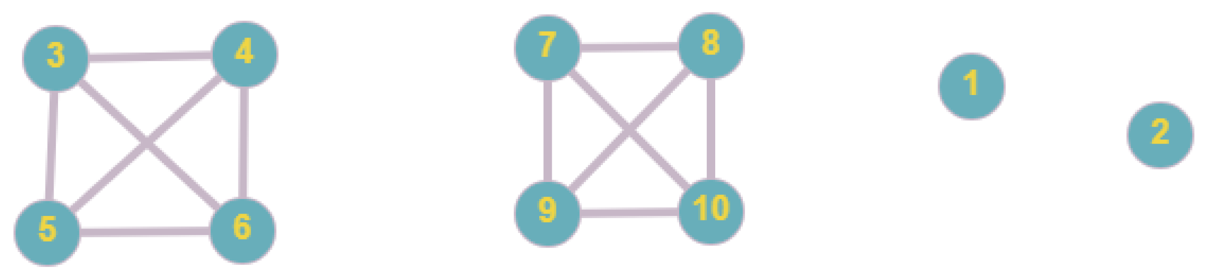
In order to measure the accuracy of Algorithm 2, it is necessary to take the model (1)–(3), and according to the decomposition in Figure 5, construct a special example using additional parameters. These parameters must be related to the number of generated operations N described in the beginning of Section 3. It is necessary to describe these parameters in such a way that this special case is the worst case for the Algorithm 2. The estimate of the accuracy in the worst case will be the accuracy of the algorithm. For Algorithm 1, everything is done similarly, but instead of a decomposition graph, each operation is considered separately and then there is a balancing process according to Steps 2 and 3 of Algorithm 1.

Worst case of Algorithm 1. The problem of calculating the absolute error for the NP-hard problem is quite time consuming. The study of this problem is planned to be covered in future papers. However, let us show a rough estimation of the algorithm accuracy without taking into account some restrictions existing in practice. Let us neglect the restriction on the total number of operations and the number of operations that are assigned to each operation to construct the worst case of the problem. The exact algorithm allows for an even distribution of operations between operations, so we will construct the worst-case example so that the distribution of operations is unequal. Furthermore, the exact algorithm allows you to go through all possible combinations, to construct the worst case so that the approximate algorithm works least accurately due to the order of operations of the different durations. To increase the error of the approximate algorithm we will use only the minimum and maximum operations. In our case, the minimum duration of the operation is $h=1$ h, and the maximum is $H=6$ h. We took these durations based on historical data. Furthermore, we use the restriction on the size of one day in the operating room–$A=11$ h of work. We construct the jobs in such a way that by using the largest duration of the surgery in each working day we get the gaps of a maximum size. Let the next set of surgeries be assigned to the first department for this week: eight surgeries with a duration of $A/2$ h, 180 surgeries with a duration of h hours, and 36 surgeries with a duration of H hours. Furthermore, the rest of the departments are empty. Following the exact approach, the schedule will be constructed as follows: all surgeries of $A/2$ h will be assigned to the first operating room (two surgeries for each day). Furthermore, the rest of the operating rooms will have one surgery of a duration of H and five surgeries of a duration of h on each day. Thus, there will be no gaps in the schedule at all. Applying the first algorithm to this example yields the following results: Since at the first step of the algorithm we construct the schedule for all departments separately, all surgeries of $A/2$ h will be assigned to the first operating room, but then all other surgeries will be on the waiting list. According to the second and third steps of Algorithm 1 on page 9, the operations from the waiting list will be distributed as follows: operating rooms number 2, 3, 4, and 5 will be “packed” with surgeries of a duration of $h=1$ h, this will require $\frac{4·A·D}{h}=176$ surgeries, where $D=4$ days. The remaining four surgeries of a duration of h will be assigned to OR six on the first day. Finally, one surgery of a duration of H will be assigned to operating room numbers 6, 7, 8, 9, and 10 for each day. So, it turns out that the number of gap hours is equal to $M^{\prime }·D·(A-H)-4=96$ h, where $M^{\prime }=5$ it is the number of not-fully-filled operating rooms. As a result, we obtain that a rough estimate of the absolute error of Algorithm 1 is 96 h.

Worst case of Algorithm 2. To construct the worst case for Algorithm 2, we introduce an additional restriction: 10 to 20 patients must be admitted to each department. Without this restriction, Algorithm 2 does not make much sense for extreme cases. To construct the worst case, we distribute the surgeries as follows: In each department of the first subgraph of the decomposition graph in Figure 5, we place 10 surgeries of duration $(A-H)=5$ h. Furthermore, in each department of the second subgraph we place 10 surgeries of duration $H=6$ h. We also place 10 surgeries of duration $(A-H)$ hours and 10 surgeries of duration H hours, respectively, in department one and two. Thus, the exact approach would give an optimal solution with the number of gap hours equal to zero: each operating room would have one surgery of duration $(A-H)$ and one surgery of duration H on each day. Furthermore, following Algorithm 2, we obtain that half of the operating rooms for each day have one surgery of duration H, and the other half of the operating rooms for each day have two surgeries of duration $(A-H)$. We get the following estimate of the absolute error of gap hours for Algorithm 2:

$$Ga{p}_{abs}=\frac{M}{2}·D·(A-H)+\frac{M}{2}·D·(A-2(A-H))=\frac{M}{2}·D·H=120,$$

(10)

where M = 10—the number of operating rooms.

The result is that a rough estimate of the absolute error of Algorithm 2 is 120 h. However, although Algorithm 2 has a worse accuracy estimate, Algorithm 1 performs worse on average, as will be shown in the results below.

Our problem is a generalization of the 0–1 multiple knapsack problem. This problem is NP-hard, and it is shown in [15], where our problem is called LEGAP—a special case of the generalized assignment problem. Since it is NP-hard, it is not possible to obtain theoretical estimates for these algorithms. To estimate the practical accuracy of the algorithms, the extreme cases of the examples were constructed. In the first case, the surgeries with the minimum variation in the duration of surgeries were taken, and in the second case, with the maximum variation. 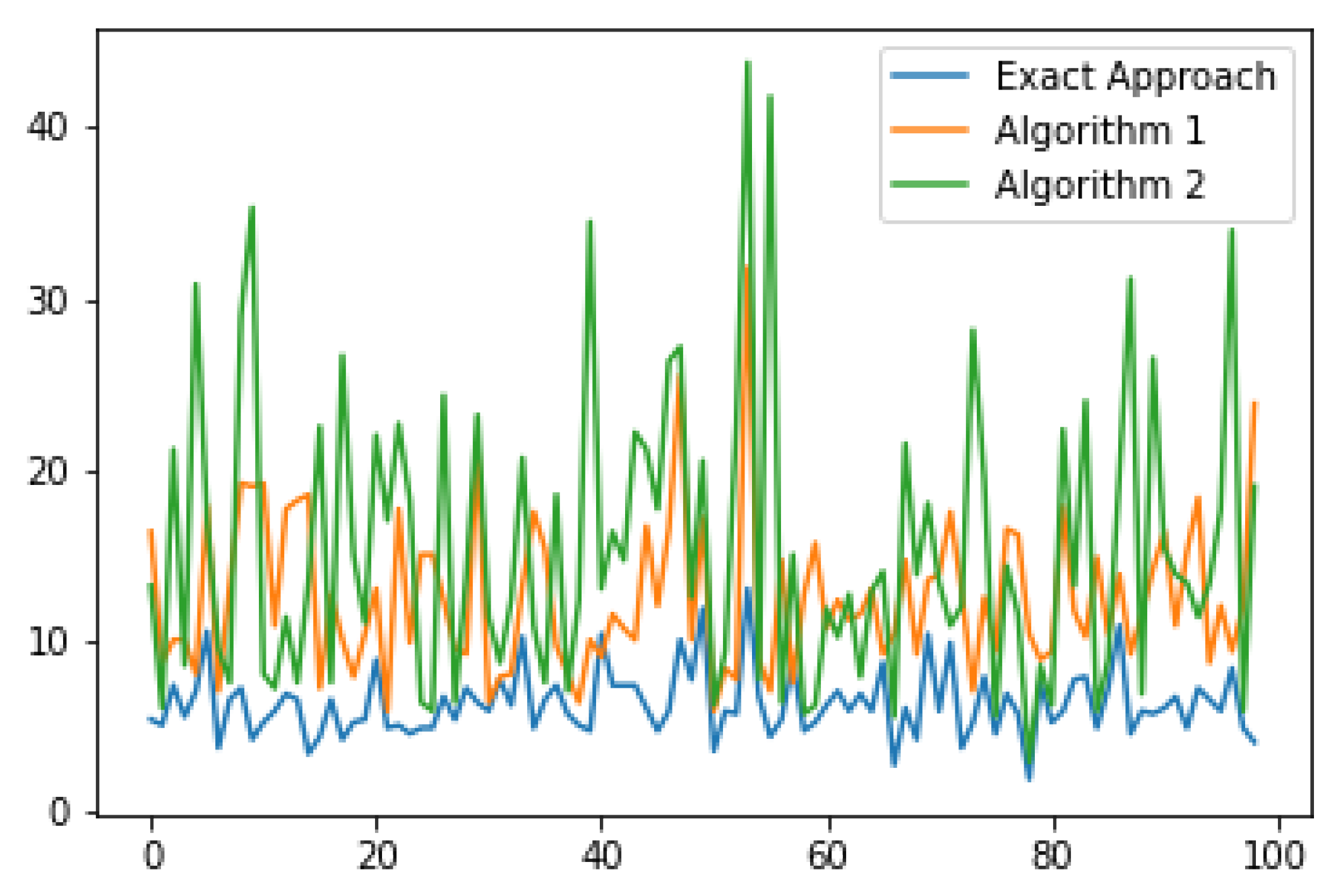As shown in [16,17], for examples with a large scatter of surgery duration, the core-type algorithms work badly, and for examples with a small scatter of surgery duration, the graphical-type algorithms work badly. For this experiment, the data were divided into two types. In the first case, the duration of the surgeries varies from 1.5 h to 9 h, with a uniform distribution. That is, the duration of surgeries has a very large scatter. In the second case, the duration of surgeries varies from 4.5 to 5.5 h, also with a uniform distribution. Using this experiment, we analyze the accuracy estimate of our algorithms depending on the width of the range of the duration of the surgeries. The other parameters of data remained the same as for the previous experiments. The assignment of surgeries to each of the 10 departments for each case is the same. However, in this experiment, half of the working week was taken, i.e., 2 days. Accordingly, half as many surgeries were taken. This was done so that the MILP solver could solve all the examples in a reasonable time. For each type, 100 examples were generated and tested for each of our approaches. 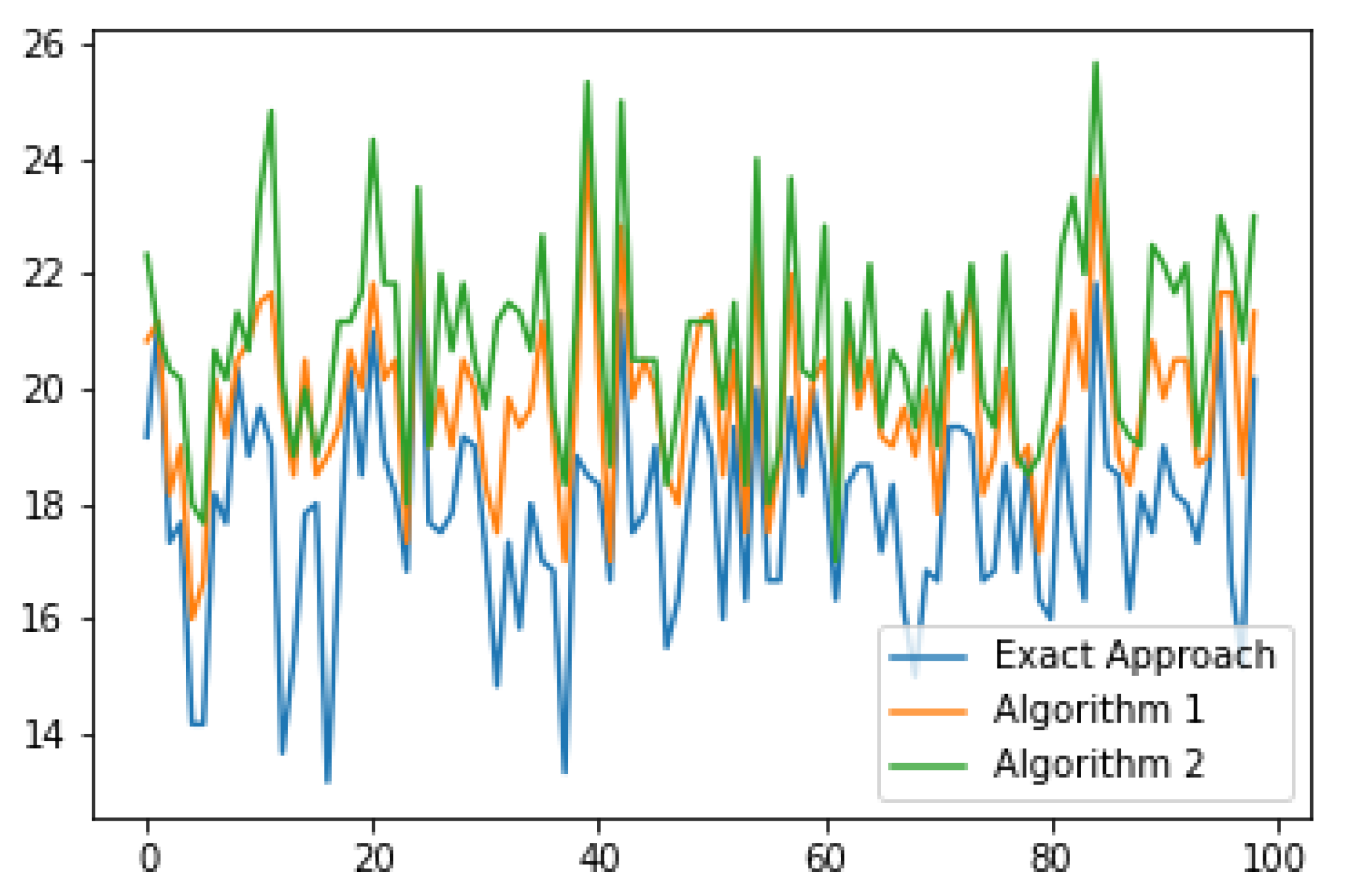Figure 6 and Figure 7 show a graph of the dependence of the gap hours in the examples with a small variation of the duration of surgeries and on the examples with a large variation of the duration, accordingly. In Figure 6, it can be seen that Algorithm 1 performs better in almost all examples compared to Algorithm 2. The absolute error of the algorithms compared to the exact approach is not very large for surgeries with a small scatter, while it is already significantly larger for surgeries with a large scatter. Furthermore, it can be noticed that the scatter of the gap hours in Figure 6 is smaller than in Figure 7, which is quite logical, since the examples in Figure 6 are close to each other.

The average values of the objective function and the number of guest surgeries are shown in

Table 1. Average values.

Data Type	Average	Exact Approach	Algorithm 1	Algorithm 2
Surgeries with a wide	Gap hours, hours	5.7	12.9	14.6
variation in duration	Guest surgeries	10.2	12.1	8.8
Surgeries with a small	Gap hours, hours	17.7	17.9	20.8
variation in duration	Guest surgeries	1.0	11.9	4.0

. In the case of surgeries with a wide variation of duration, the absolute error of the gap hours for Algorithm 1 is $7.2$ h, and for Algorithm 2 it is $8.9$ h, while the number of guest surgeries for each approach is about the same. Now consider the case of surgeries with a small variation of duration. The absolute error of the gap hours for Algorithm 1 is only $0.2$ h, and for Algorithm 2 it is $2.1$ h. However, the average number of guest surgeries is different for each approach. For the exact approach, the average number of guest surgeries is equal to one. This can be explained by the fact that in each department the duration of the surgeries is almost the same. In Algorithm 2, the number of guest surgeries is not too large either, but Algorithm 1 has an average of 12 guest surgeries. This is due to the fact that in the second and third steps of Algorithm 1, surgeries are transferred from one department to another, even with a small improvement in the objective function. To summarize, our approaches work better for surgeries with a wide range of duration. This is a good factor for us, since in real life, the durations of surgeries are very different.

5. Results

Now we need to compare all approaches on the same data. All results are present in

Table 2. Computing Time.

Experiment	Exact Approach, sec	Algorithm 1, sec	Algorithm 2, sec
1	1500	1.92	7
2	340	1.97	13
3	1350	2.35	31
4	310	2.99	21
5	150	1.91	9
6	-	2.16	13
7	-	2.15	7
8	-	2.3	11
9	-	2.2	48
10	-	2.5	15

,

Table 3. Gap hours (objective function).

Experiment	Exact Approach, Hours	Algorithm 1, Hours	Algorithm 2, Hours
1	8	18.5	9
2	6	23	16
3	7.7	22	13
4	7	20.5	11.5
5	4.8	16	9
6	-	21.5	12.5
7	-	15.5	7
8	-	17	12.5
9	-	25	13
10	-	23	8

,

Table 4. Guest surgeries.

Experiment	Exact Approach	Algorithm 1	Algorithm 2
1	17	15	9
2	12	20	13
3	16	26	13
4	13	16	13
5	14	26	7
6	-	31	12
7	-	22	13
8	-	20	13
9	-	18	8
10	-	19	10

and

Table 5. Average values.

Average	Exact Approach	Algorithm 1	Algorithm 2
Computing time, sec	730	2.2	17.5
Gap hours, hours	6.7	20.2	11.1
Guest surgeries	14.4	21.3	11.2

; “-” means that the solve time limit is exceeded. The time limit is 30 min. All 10 examples were generated in the same way described in Section 3. Furthermore, we present an example schedule with the help of Gantt charts in Figure 8. Guest surgeries are marked in black.

Figure 8 presents that there are not many guest surgeries, and the duration of the surgeries is widely scattered.

Table 2 shows the computing times for each approach for different examples. The computational time for the exact approach is extremely data-dependent. Furthermore, some examples cannot be solved at all within the time limits we set. Furthermore, the examples that are solved are solved long enough. Algorithms 1 and 2 solve the problem faster. In particular, Algorithm 1 is on average several times faster than Algorithm 2.

Table 3 compares the total number of gap hours for each approach. The results obtained by the exact algorithm show that the gaps range from 4.8 to 8 h for the groups of examples considered, but the results obtained by Algorithm 1 on average differ by 13.1 h compared to the exact approach. At the same time, the gaps obtained for the examples that the exact algorithm was unable to calculate averaged 20.4 h for Algorithm 1. Algorithm 2 in turn differs from the exact solution by 5.1 h for the first five examples. Furthermore, for the following examples, which do not have an exact solution, the gaps average 10.6 h for Algorithm 2.

Table 4 shows the number of guest surgeries. We have chosen the parameters so that the number of guest surgeries would be acceptable for each approach. It can be seen that for Algorithm 2, guest surgeries on average turn out even less than the exact approach; this is due to the decomposition of the problem into several groups of departments, while Algorithm 1 has more guest surgeries than the exact approach, because in it we transfer surgeries from one department to another at steps 2 and 3 of the algorithm.

It can be seen that the exact approach can not find the optimal solution within the time limit for all generated examples. Thus, it can be observed that algorithms have a much shorter computation time, and at the same time do not lose much in the objective function. As we can see in Table 4, Algorithm 1 is the fastest, but Algorithm 2 has a running time not much longer and the objective function is half the size of Algorithm 1. However, pay attention to the gap hours relative to all available work times of all ORs in these two weeks. There are 880 h of work time. Furthermore, even in Algorithm 1, the gap hours are only $2.3\%$ of all work time. It is not much different from the optimal solution with $0.8\%$.

6. Conclusions

This paper presents a formal statement of the problem of the predictive planning of surgery units in a large medical hospital and outlines the methods for its optimal solution. The experiments were carried out on real data that was generated based on data provided by the Burdenko Institute. The managerial insights of this work are to implement a program for scheduling operating rooms to automate this process and increase patient throughput at the Burdenko Neurosurgical Center. To achieve this, the plan is to make the existing model more complex, so that it is as similar as possible to the real situation in the hospital. In future works, we plan to add the uncertainty of the duration of surgery, urgent patients, and the work of anesthesiologists.

The hospital report shows some departments are busier than others. Furthermore, our model implies the possibility of transferring the patients to the operating rooms of other departments if they are not busy. Our main goal was to increase patient throughput. This can be achieved by maximizing the number of operating hours. Operating rooms should be out of work for as little time as possible. The MILP model allows us to construct a long-term schedule with fewer gaps. Since we have to make a new schedule every time a patient is removed or added to the waiting list, a new schedule should be made in a short period of time. Furthermore, since our model is computationally complex, two decomposition algorithms were presented that significantly reduce the time calculations.

This paper shows that the complexity of the proposed algorithms is significantly reduced compared to the complexity of the exact approach. This thesis is confirmed in practice: the exact solution was obtained only in half of the cases. The problem with the exact approach is that for cases with the same number of applications but different distributions of surgery durations across operating rooms this approach may not find an exact solution in an acceptable time. Discussions are carried out regarding the theoretical estimation of the accuracy of the algorithms. For those examples for which the exact solution was obtained, the relative error of the solution was calculated. It can be seen that the first algorithm is further from the exact solution than the second. For further examples, in the accuracy of which has not been estimated we can also see this pattern. The objective function value obtained by the first algorithm is much higher than for the second. At the same time, we see that the computation time for the first algorithm is much less than for the second. This paper contributes to solving the problem of scheduling operating rooms. The peculiarity of the problem is that the operating rooms are multidisciplinary. That is, the operating rooms are assigned to certain departments where patients are admitted. The MILP model was invented for this problem. This problem is NP-hard. Therefore, it took a long time to construct the schedule. To solve this problem, two decomposition algorithms were developed to reduce the solution time. Furthermore, the complexities and rough estimates of the accuracies of these algorithms are given. In the future, we plan to expand the model for emergency patients and to add uncertainty, and we also will try a metric approach [18] for this case.

References

1. Zhu, S.; Fan, W.; Yang, S.; Pei, J.; Pardalos, P.M. Operating room planning and surgical case scheduling: A review of literature. J. Comb. Optim. 2019, 37, 757–805. [Google Scholar] [CrossRef]
2. Rahimi, I.; Gandomi, A.H. A Comprehensive Review and Analysis of Operating Room and Surgery Scheduling. Arch. Comput. Methods Eng. 2021, 28, 1667–1688. [Google Scholar] [CrossRef]
3. Clavel, D.; Mahulea, C.; Albareda, J.; Silva, M. A decision support system for elective surgery scheduling under uncertain durations. Appl. Sci. 2020, 10, 1937. [Google Scholar] [CrossRef] [Green Version]
4. Rivera, G.; Cisneros, L.; Sánchez-Solís, P.; Rangel-Valdez, N.; Rodas-Osollo, J. Genetic algorithm for scheduling optimization considering heterogeneous containers: A real-world case study. Axioms 2020, 9, 27. [Google Scholar] [CrossRef] [Green Version]
5. Allen, T.T.; Hernandez, O.K.; Roychowdhury, S.; Patterson, E.S. Practical Optimal Scheduling for Surgery. In Proceedings of the International Symposium on Human Factors and Ergonomics in Health Care; Sage: Los Angeles, CA, USA, 2020; Volume 9, pp. 1–14. [Google Scholar] [CrossRef]
6. Shylo, O.V.; Prokopyev, O.A.; Schaefer, A.J. Stochastic operating room scheduling for high-volume specialties under block booking. INFORMS J. Comput. 2013, 25, 682–692. [Google Scholar] [CrossRef] [Green Version]
7. Gür, Ş.; Eren, T.; Alakaş, H.M. Surgical operation scheduling with goal programming and constraint programming: A case study. Mathematics 2019, 7, 251. [Google Scholar] [CrossRef] [Green Version]
8. Lin, Y.K.; Li, M.Y. Solving Operating Room Scheduling Problem Using Artificial Bee Colony Algorithm; Healthcare Multidisciplinary Digital Publishing Institute: Basel, Switzerland, 2021; Volume 9, p. 152. [Google Scholar] [CrossRef]
9. Kayvanfar, V.; Akbari Jokar, M.R.; Rafiee, M.; Sheikh, S.; Iranzad, R. A new model for operating room scheduling with elective patient strategy. INFOR Inf. Syst. Oper. Res. 2021, 59, 309–332. [Google Scholar] [CrossRef]
10. Naderi, B.; Roshanaei, V.; Begen, M.A.; Aleman, D.M.; Urbach, D.R. Increased surgical capacity without additional resources: Generalized operating room planning and scheduling. Prod. Oper. Manag. 2021, 30, 2608–2635. [Google Scholar] [CrossRef]
11. Hans, E.; Wullink, G.; Van Houdenhoven, M.; Kazemier, G. Robust surgery loading. Eur. J. Oper. Res. 2008, 185, 1038–1050. [Google Scholar] [CrossRef]
12. Pang, B.; Xie, X.; Song, Y.; Luo, L. Surgery scheduling under case cancellation and surgery duration uncertainty. IEEE Trans. Autom. Sci. Eng. 2018, 16, 74–86. [Google Scholar] [CrossRef]
13. Liu, H.; Zhang, T.; Luo, S.; Xu, D. Operating room scheduling and surgeon assignment problem under surgery durations uncertainty. Technol. Health Care 2018, 26, 297–304. [Google Scholar] [CrossRef] [PubMed]
14. Lazarev, A.A.; Lemtyuzhnikova, D.V.; Mandel, A.S.; Pravdivets, N.A. The Problem of the Hospital Surgery Department Debottlenecking In International Conference on Learning and Intelligent Optimization; Springer: Cham, Germany, 2020; pp. 289–302. [Google Scholar] [CrossRef]
15. Ohlsson, M.; Pi, H. A study of the mean field approach to knapsack problems. Neural Netw. 1997, 10, 263–271. [Google Scholar] [CrossRef]
16. Hans, K.; Ulrich, P.; David, P. Knapsack Problems; Springer Science & Business Media: Berlin/Heidelberg, Germany, 2004; ISBN 10:3540402861/ISBN 13:9783540402862. [Google Scholar]
17. Lazarev, A.A.; Werner, F. A graphical realization of the dynamic programming method for solving NP-hard combinatorial problems. Comput. Math. Appl. 2009, 58, 619–631. [Google Scholar] [CrossRef] [Green Version]
18. Lazarev, A.A.; Lemtyuzhnikova, D.V.; Werner, F. A metric approach for scheduling problems with minimizing the maximum penalty. Appl. Math. Model. 2021, 89, 1163–1176. [Google Scholar] [CrossRef]
Figure 1. The dependency of the total duration of all schedule gaps on the weight w 0 , 1 w o 100 .
Mathematics 10 00784 g001
Figure 2. More detailed dependency diagram of the total duration of all schedule gaps on the weight w 0 , 1 w o 10 .
Mathematics 10 00784 g002
Figure 3. The dependency of the number of guest surgeries on the weight w 0 , 1 w o 100 .
Mathematics 10 00784 g003
Figure 4. More detailed dependency diagram of the number of guest surgeries on the weight w 0 , 1 w o 10 .
Mathematics 10 00784 g004
Figure 5. Decomposition graph.
Mathematics 10 00784 g005
Figure 6. Graph of the dependence of the gap hours on the examples with a small variation of the duration.
Mathematics 10 00784 g006
Figure 7. Graph of the dependence of the gap hours on the examples with a large variation of the duration.
Mathematics 10 00784 g007
Figure 8. Example of schedule for exact approach.
Mathematics 10 00784 g008