Changing the Threshold in a Bivariate Polynomial Based Secret Image Sharing Scheme

Abstract

Secret image sharing (SIS) is an important application of the traditional secret sharing scheme, which has become popular in recent years. In an SIS scheme, a confidential image is encrypted into a group of shadows. Any set of shadows that reaches the threshold can reconstruct the image; otherwise, nothing can be recovered at all. In most existing SIS schemes, the threshold on shadows for image reconstruction is fixed. However, in this work, we consider more complicated cases of SIS, such that the threshold is changeable according to the security environment. In this paper, we construct a $(k\leftrightarrow h,n)$ threshold-changeable SIS (TCSIS) scheme using a bivariate polynomial, which provides $h-k+1$ possible thresholds, $k,k+1,\dots ,h$. During image reconstruction, each participant can update their shadow according to the current threshold T based only on their initial shadow. Unlike previous TCSIS schemes, the proposed scheme achieves unconditional security and can overcome the information disclosure problem caused by homomorphism.

1. Introduction

The issue of image security has become important in recent years—for instance, in image steganography [1,2] and verification of visual consistency of images [3]. Secret image sharing (SIS) is also an important topic in image security, which is meant to protect confidential images among multiple participants. Most SIS schemes satisfy a $(k,n)$ threshold, such that an image is encrypted into n shadows: k or more shadows can reconstruct the image, but less than k shadows can do nothing. There are two main approaches for SIS: visual cryptography-based SIS schemes [4,5,6] and polynomial-based SIS schemes [7,8,9]. Visual cryptography-based SIS uses the human visual system to recover an image, but the shadow size is greatly expanded from the original image, and the reconstructed image is of diminished quality; polynomial-based SIS is capable of recovering an image losslessly, and the shadow size is reduced from the original image, but the computation for image reconstruction is more complicated than in visual cryptography-based SIS. Many research topics concerning SIS exist, such as progressive SIS [10,11,12], SIS with essential shadows [13,14], and SIS with authentication [15]. When an image has a huge number of pixels, the computations in shadow generation or image reconstruction may cause high time complexity. One can use the method of compressive sensing [16,17] to reduce image size, so that the time complexity for an SIS scheme can be reduced.

Most existing SIS schemes consider a single security policy, and the threshold k for image reconstruction is fixed. However, the security environment for image reconstruction is probably changeable in real applications; therefore, it is more reasonable to design SIS schemes with the capability of threshold changeability. The considerations for threshold changeability include: (1) the security level of a secret image may change; (2) the number of total participants may vary; (3) the power of adversaries may increase; (4) information disclosure may be caused by some malicious participants. Discussion on changing thresholds in traditional secret sharing [18,19,20] has already been presented, which proves the necessity for threshold changeability in SIS. However, SIS and traditional secret sharing are different. The studies on threshold-changeable secret sharing could not be directly copied into TCSIS. In fact, the discussion on TCSIS is insufficient in the literature. Two TCSIS schemes [21,22] have been constructed. In the first TCSIS scheme [21], there are N possible thresholds $T_1,T_2,\dots ,T_N$, but extra two-variable one-way functions are included for image reconstruction. The computational complexity is high, and the security is based on the assumption of one-way functions. It is unconditionally secure. The other TCSIS scheme [22] has reduced computational complexity, but it has only three possible thresholds $(k^{{}^{\prime }},k,k^{{}^{″}})$. In addition, it requires the dealer to be involved in shadow updating, and it suffers from the problem of information leakage.

In this paper, we construct a $(k\leftrightarrow h,n)$ TCSIS scheme which provides $h-k+1$ possible thresholds, $(k,k+1,\dots ,h-1,h)$. The shadows are encrypted using a bivariate polynomial, and the participant only keeps one initial shadow from the dealer. During image reconstruction, the dealer or another trusted party chooses a threshold T from $\{k,k+1,\dots ,h\}$ according to the current security requirement; then, each participant can update their shadow according to threshold T. In addition, the process of shadow updating is only based on the initial shadow. The dealer does not need to participate in this process. All the computations in the proposed scheme are polynomial, making them highly efficient.

The rest of this paper is organized as follows. In next section, some preliminaries are prepared which include the Thien–Lin polynomial-based $(k,n)$ SIS and some results of previous TCSIS. Our proposed scheme is described in Section 3 together with the corresponding theoretical proofs. Comparisons between the proposed scheme and previous TCSIS schemes and experimental results are shown in Section 4. The conclusions of our work are presented in Section 5.

2. Related Works

In this section, we briefly introduce some related studies about TCSIS, which relate to polynomial-based SIS, the model of TCSIS, and one previous TCSIS.

2.1. Polynomial Based SIS

The model of $(k,n)$ SIS consists of two phases, which can be shown as follows.

Model of SIS

Shadow Encryption Phase

1

A dealer encrypts a confidential image O into shadows $S_1,S_2,\dots ,S_n$.

2

Each shadow $S_i$ is sent to participant ${\mathcal{P}}_i$ through a secure channel.

Image Reconstruction Phase

Any set of k or more participants can reconstruct the image O; less than k participants cannot get any information on the image at all.

In 2002, Thien and Lin proposed a polynomial based $(k,n)$ threshold SIS scheme [7], which was the foundation for later polynomial based SIS schemes. All existing TCSIS schemes were based on the Thien–Lin polynomial-based SIS, and our work is also inspired by their work. Therefore, it is necessary to give a description of their work.

Scheme 1: Thien–Lin $(k,n)$ SIS

Shadow Encryption Phase:

Input: image O, Output: n shadows $S_1,S_2,\dots ,S_n$

1

The dealer divides O into l-non-overlapping k-pixel groups, $G_1,G_2,\dots ,G_l$.

2

For k pixels $p_{j,0},p_{j,1},\dots ,p_{j,k-1}$ in each group $G_j,j\in [1,l]$, the dealer builds a $k-1$ degree polynomial $f_j\left(x\right)=p_{j,0}+p_{j,1}x+p_{j,2}{x}^2+\dots ,+p_{j,k-1}{x}^{k-1}$.

3

The dealer computes n sub-shadows, $s_{j,1}=f_j\left(1\right),s_{j,2}=f_j\left(2\right),\dots ,s_{j,n}=f_j\left(n\right),j\in [1,l]$.

4

The dealer outputs n shadows $S_i=s_{1,i}\Vert s_{2,i}\Vert ,\dots ,\Vert s_{l,i},i=1,2,\dots ,n$.

Image Reconstruction Phase:

Input: m shadows $S_1,S_2,\dots ,S_m$.$(m\ge k)$. Outputs: secret image O.

1

Reconstructing $f_j\left(x\right)$ from $s_{1,j},s_{2,j},\dots ,s_{m,j},j\in [1,l]$ using Lagrange interpolation:

$$f_j\left(x\right)=\sum _{i=1}^m[s_{i,j}\times \prod _{w=1,w\ne i}^m\frac{x-w}{i-w}];$$

(1)

then the block $G_j$ is recovered from all k coefficients in $f_j\left(x\right)$.

2

Output: $O=G_1\Vert G_2\Vert ,\dots ,\Vert G_l$.

2.2. Results on TCSIS

In this section, we give a model of TCSIS, and then describe some results on previous TCSIS schemes.

The model TCSIS scheme consists of two phases: shadow encryption phase and image reconstruction phase, which have the following steps.

Model of TCSIS

Shadow Encryption Phase

1

A dealer encrypts a confidential image O into initial shadows $S_1,S_2,\dots ,S_n$.

2

Each initial shadow $S_i$ is sent to participant ${\mathcal{P}}_i$ through secure channel.

Image Reconstruction Phase

1

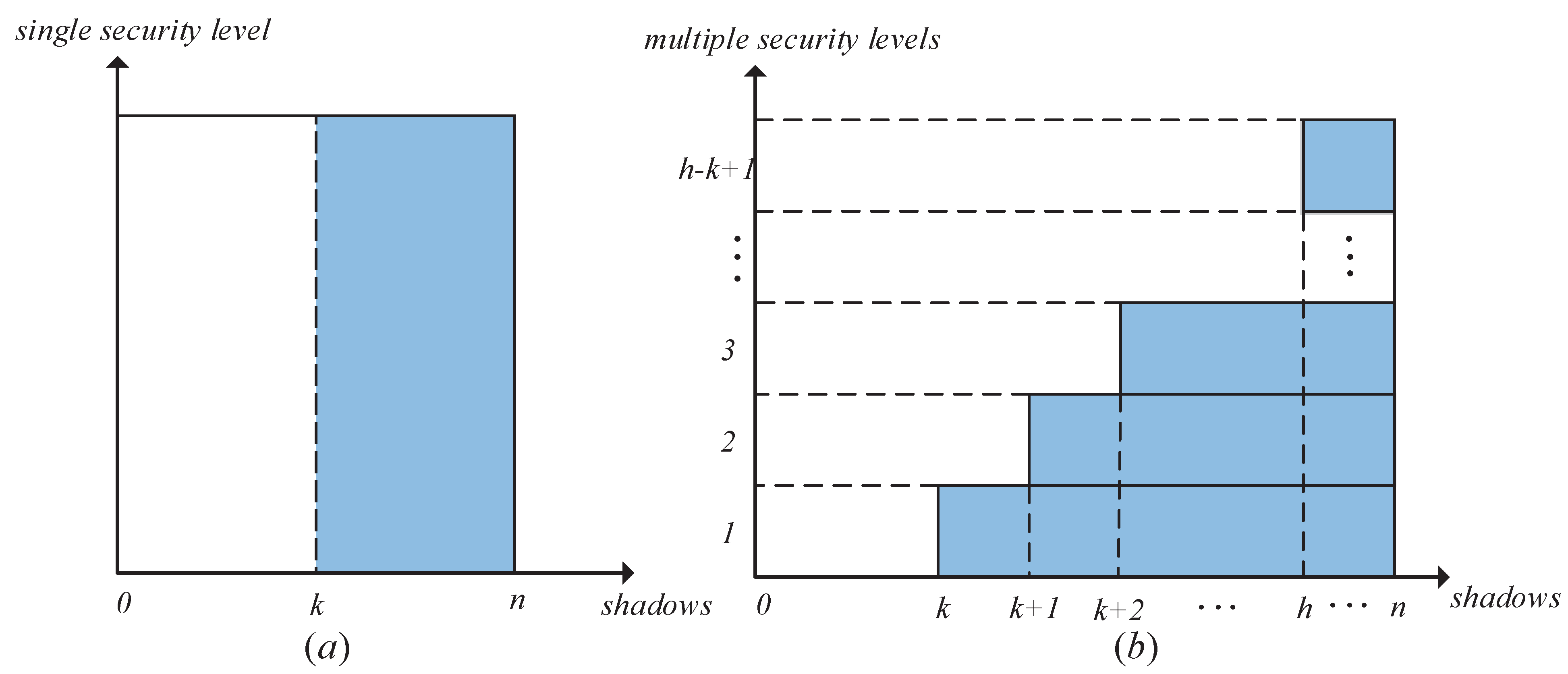
A threshold T is selected from the set of all possible thresholds $T_1,T_2,\dots ,T_d$.

2

Each participant ${\mathcal{P}}_i$ updates the shadow according to current threshold T.

3

Any group of participants that satisfy the access structure can reconstruct the image O using updated shadows.

The difference between the SIS model and the TCSIS model is that during the the image reconstruction phase, each participant needs to update the shadow according to the current threshold T.

The scheme in [21] is a polynomial scheme that satisfies the model of TCSIS; however, some one-way functions were adopted in [21] to change the threshold. Therefore, the security of [21] is based on the security assumptions of those one-way functions, and the computational complexity is much higher than the computations in polynomial interpolation. Recently, Liu et al. proposed a $(k^{{}^{\prime }},k,k^{{}^{″}})$ TCSIS [22] that can reduce the computational complexity of [21]. However, there are only three available thresholds in [22], and the dealer has to involve one in shadow updating. In addition, information leakage can occur in [22] due to the property of homomorphism. Since the scheme in [22] is more representative than the scheme in [21], we give a description of the scheme in [22] in the following.

Scheme 2: Liu et al.’s $(k^{{}^{\prime }},k,k^{{}^{″}})$ TCSIS [22]

Shadow Encryption Phase:

1

The dealer $\mathcal{D}$ divides an image O into l non-overlapping $k^{{}^{\prime }}$ pixel blocks, $G_1,G_2,\dots ,G_l$.

2

For $k^{{}^{\prime }}$ pixels $p_{j,0},p_{j,1},\dots ,p_{j,k^{{}^{\prime }}-1}$ in each block $G_j,j\in [1,l]$, $\mathcal{D}$ generates a $k^{{}^{\prime }}-1$ degree polynomial $f_j\left(x\right)=p_{j,0}+p_{j,1}x+p_{j,2}{x}^2+\dots ,+p_{j,k^{{}^{\prime }}-1}{x}^{k^{{}^{\prime }}-1}$.

3

$\mathcal{D}$ selects randomly $k-k^{{}^{\prime }}$ integers $w_{k^{{}^{\prime }}},w_{k^{{}^{\prime }}+1},\dots ,w_{k-1}$, and generates a $k-1$ degree polynomials $F^{{}^{\prime }}\left(x\right)=w_{k^{{}^{\prime }}}{x}^{k^{{}^{\prime }}}+w_{k^{{}^{\prime }}+1}{x}^{k^{{}^{\prime }}+1}+\dots +w_{k-1}{x}^{k-1}$. In addition, $\mathcal{D}$ randomly selects $k^{{}^{″}}-k$ integers $r_k,r_{k+1},\dots ,r_{k^{{}^{″}}-1}$ and generates a polynomial: $F^{{}^{″}}\left(x\right)=r_k{x}^k+r_{k+1}{x}^{k+1}+\dots +r_{k^{{}^{″}}-1}{x}^{k^{{}^{″}}-1}$.

3

Let $F_j\left(x\right)=f_j\left(x\right)+F^{{}^{\prime }}\left(x\right)$. $\mathcal{D}$ computes n sub-shadows $s_{j,1}=F_j\left(1\right),s_{j,2}=F_j\left(2\right),\dots ,s_{j,n}=F_j\left(n\right),j\in [1,l]$, and the initial shadow $S_i$ of ${\mathcal{P}}_i$ is $S_i=s_{1,i}\Vert s_{2,i}\Vert ,\dots ,\Vert s_{l,i},i=1,2,\dots ,n$.

Image Decryption Phase:

$\mathcal{D}$ chooses a threshold from $\{k^{{}^{\prime }},k,k^{{}^{″}}\}$ and publishes it to all participants.

1

If the threshold is k, k or more initial shadows can reconstruct l polynomials $F_j\left(x\right),j=1,2,\dots ,l$. $k^{{}^{\prime }}$ pixel block $G_j$ is made up of the first $k^{{}^{\prime }}$ coefficients in $F_j\left(x\right)$, and thus the image $O=G_1\left|\right|G_2\left|\right|\dots \left|\right|G_l$ can be recovered.

2

If the threshold is $k^{{}^{\prime }}$, $\mathcal{D}$ publishes the information of $e_i=F^{{}^{\prime }}\left(i\right),i=1,2,\dots ,n$ to all participants. Each participant ${\mathcal{P}}_i$ updates its shadow by: $S_i^{k^{{}^{\prime }}}=L_i\left(S_i\right)=S_i-e_i$. Here the operation of $S_i-e_i$ is defined as:$S_i-e_i=(s_{1,i}-e_i)\left|\right|(s_{2,i}-e_i)\left|\right|\dots \left|\right|(s_{l,i}-e_i)$. Let $P^{{}^{\prime }}=\left\{S_i^{k^{{}^{\prime }}}\right|i=1,2,\dots ,n\}$. The threshold of all updated shadows in $P^{{}^{\prime }}$ is decreased to $k^{{}^{\prime }}$ from k.

3

If the threshold is $k^{{}^{″}}$, $\mathcal{D}$ publishes the information of $m_i=F^{{}^{″}}\left(i\right),i=1,2,\dots ,n$. Each participant ${\mathcal{P}}_i$ updates their shadow by $S_i^{k^{{}^{″}}}=H_i\left(S_i\right)=S_i+m_i$. Here the operation of $S_i+m_i$ is defined as: $S_i+m_i=(s_{1,i}+m_i)\left|\right|(s_{2,i}+m_i)\left|\right|\dots \left|\right|(s_{l,i}+m_i)$. Let $P^{{}^{″}}=\left\{S_i^{k^{{}^{″}}}\right|i=1,2,\dots ,n\}$. The threshold of all updated shadows in $P^{{}^{″}}$ is increased to $k^{{}^{″}}$ from k.

Here we omit the process of image reconstruction with the threshold $k^{{}^{\prime }}$ and $k^{{}^{″}}$. The details can be found in reference [22].

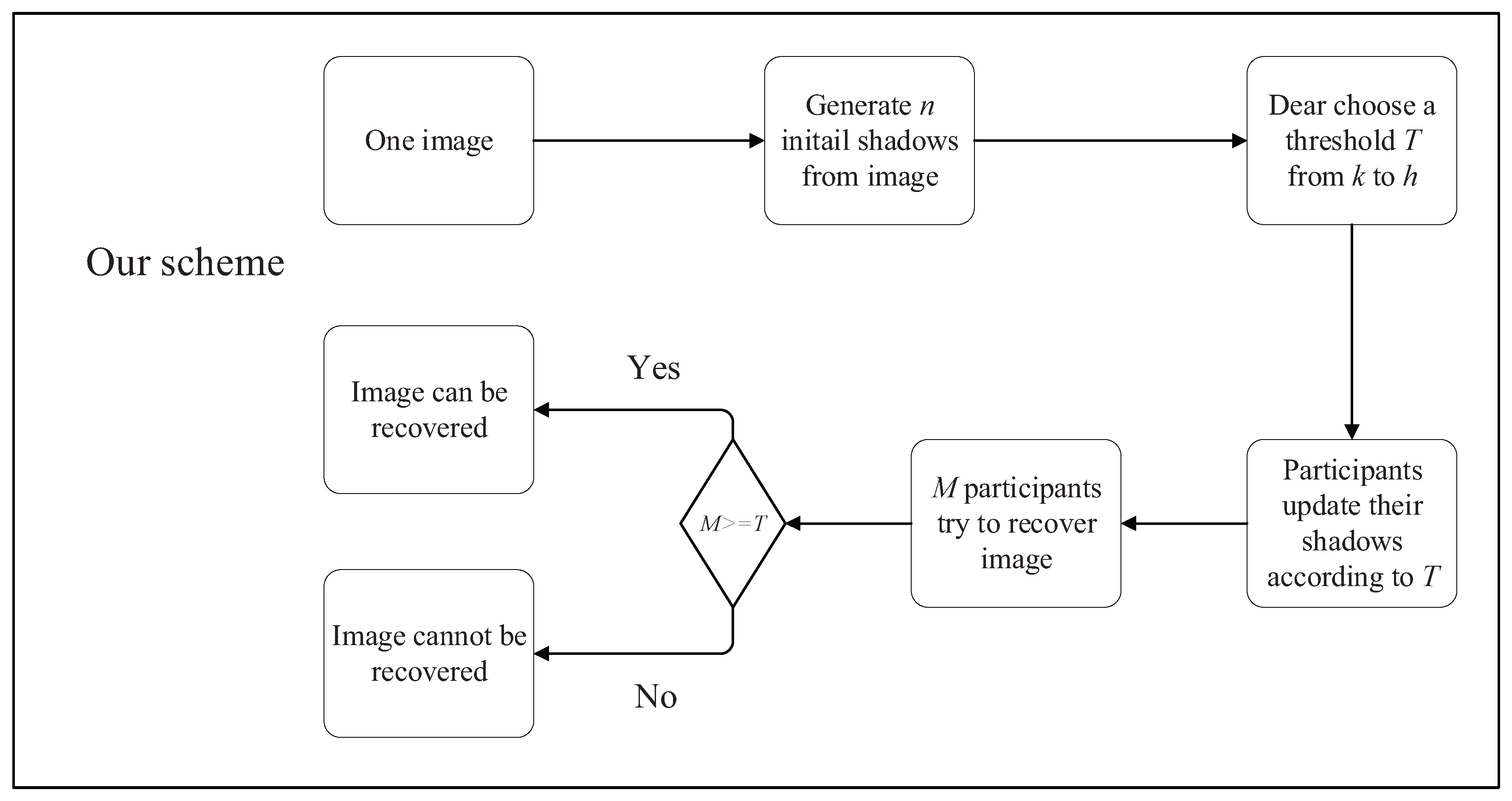
3. Proposed Scheme

3.1. Design Motivation

In real applications, security conditions are probably changeable after the dealer sends shadows in an SIS scheme to all participants. For instance, (1) the security level of a secret image may change; (2) the number of total participants may vary; (3) the power of adversaries may increase; (4) information disclosure may be caused by some malicious participants. A wide variety of emergencies can affect security requirements. In this work, we assume there are multiple security levels for image reconstruction. For instance, a confidential image should be reconstructed immediately due to emergency cases, such as in medical or traffic settings. However, if the number of available participants did not satisfy the access structure for image reconstruction, it would cause losses, even loss of life. Therefore, an SIS scheme with the capability of changing its threshold is more reasonable, since it can reconstruct images under multiple security levels. The design concept of our work can be seen in Figure 1, and the flow chart of our scheme is shown in Figure 2.

3.2. TCSIS Using a Bivariate Polynomial

The previous TCSIS schemes [21,22] were based on univariate polynomials. Differently from their works, the proposed $(k\leftrightarrow h,n)$ TCSIS is based on a bivariate polynomial, and it can provide $h-k+1$ available thresholds $\{k,k+1,\dots ,h\}$. The advantages of our scheme are that the dealer does not need to be involved in shadow updating, and that it is unconditionally secure. Similarly to the previous TCSIS schemes, the proposed scheme also divides an image into non-overlapping blocks, and each block includes $kh$ pixels. During shadow encryption phase, each block is encrypted into shadows using the same algorithm. During the image reconstruction phase, all blocks are recovered from their shadows using same algorithm. When all blocks are recovered, the image is reconstructed accordingly. Therefore, for simplicity and readability, we use a $kh$-pixels block G instead of an image, as follows.

Scheme 3: $(k\leftrightarrow h,n)$ TCSIS

Shadow Encryption Phase:

1

Suppose $p_{i,j},i=0,1,\dots ,k-1,j=0,1,\dots ,h-1$ are $kh$ pixels in G, $\mathcal{D}$ builds a bivariate polynomial:

$$F(x,y)=\left\{\begin{array}{c}{p}_{0,0}+p_{0,1}y+,\dots ,+p_{0,h-1}{y}^{h-1},\hfill \\ p_{1,0}x+p_{1,1}xy+,\dots ,+p_{1,h-1}x{y}^{h-1},\hfill \\ \dots \hfill \\ p_{k-1,0}{x}^{k-1}+p_{k-1,1}{x}^{k-1}y+,\dots ,+p_{k-1,h-1}{x}^{k-1}{y}^{h-1}\hfill \end{array}\right.$$

(2)

2

$\mathcal{D}$ computes $f_i\left(y\right)=F(i,y),g_i\left(x\right)=F(x,i)$. The initial shadow $s_i$ for ${\mathcal{P}}_i$ is $s_i=(f_i\left(y\right),g_i\left(x\right))$.

Image Reconstruction Phase:

1

Select a threshold T from the set $\{k,k+1,\dots ,h\}$.

(a)

If current threshold is $T=k$, each participant ${\mathcal{P}}_i$ updates their shadow by $s_i^k=f_i\left(y\right)$.

(b)

If the current threshold is $T=h$, each participant ${\mathcal{P}}_i$ updates its shadow by $s_i^h=g_i\left(x\right)$.

(c)

If the current threshold T satisfies $k<T<h$, the participants select $h-T$ integers $e_1,e_2,\dots ,e_{h-T}$ other than $1,2,\dots ,n$. Each participant ${\mathcal{P}}_i$ computes $f_i\left(e_1\right),f_i\left(e_2\right),\dots ,f_i\left(e_{h-T}\right)$, and the updated shadow $s_i^T$ is

$s_i^T=(s_i^h,(f_i\left(e_1\right),f_i\left(e_2\right),\dots ,f_i\left(e_{h-T}\right))$.

2

Any group of T participants can reconstruct all $kh$ pixels in G using Lagrange interpolation.

Scheme 3 describes the algorithms for updating shadows according to different thresholds, but the methods for image reconstruction using updated shadows are not given. In the following three theorems, we will prove that the updated shadows are consistent with the current threshold. This is also a proof of the security of our scheme. The methods of image reconstruction using these updated shadows are also described in these theorems.

Theorem 1.

The threshold T for updated shadows $s_1^k,s_2^k,\dots s_n^k$ on G is $T=k$.

Proof. 

According to Scheme 3, the updated shadow in $s_i^k$ for G is $s_i^k=f_i\left(y\right)=F(i,y)$. $F(x,y)$ in Equation (2) can be rewritten as:

$$F(x,y)=u_0\left(x\right)+u_1\left(x\right)y+u_2\left(x\right)y^2+,\dots ,+u_{h-1}\left(x\right)y^{h-1}$$

(3)

where $u_0\left(x\right),u_1\left(x\right),\dots ,u_{h-1}\left(x\right)$ are all $k-1$ degree univariate polynomials. Suppose that

$$s_i^k=F(i,y)=b_{i,0}+b_{i,1}y+,\dots ,b_{i,h-1}{y}^{h-1},i=1,2,\dots ,n$$

(4)

Comparing Equation (3) with Equation (4), we can observe that $(b_{1,0},b_{2,0},\dots ,b_{n,0})$ are interpolations on $u_0\left(x\right)$ that $b_{i,0}=u_0\left(i\right),i=1,2,\dots ,n$. Since $u_0\left(x\right)$ is $k-1$ degree polynomial, the threshold of $(b_{1,0},b_{2,0},\dots ,b_{n,0})$ to reconstruct $u_0\left(x\right)$ is k, and the reconstruction can be executed using Lagrange interpolation, Equation (1). As each $b_{i,0}$ comes from sub-shadow $s_i^k$, the threshold on $(s_1^k,s_2^k,\dots ,s_n^k)$ for $u_0\left(x\right)$ is k. By the same way, the threshold for the other polynomials $u_1\left(x\right),u_2\left(x\right),\dots ,u_{h-1}\left(x\right)$ on $(s_1^k,s_2^k,\dots ,s_n^k)$ is also k. In summary, the threshold for the $kh$ pixel block G from $(s_1^k,s_2^k,\dots ,s_n^k)$ is $T=k$. □

Theorem 2.

The threshold T for updated shadows $s_1^h,s_2^h,\dots ,s_n^h$ is $T=h$.

Proof. 

The updated shadow $s_i^h$ for G is $s_i^h=g_i\left(x\right)=F(x,i)$. $F(x,y)$ in Equation (2) can be rewritten as:

$$F(x,y)=v_0\left(y\right)+v_1\left(y\right)x+v_2\left(y\right)x^2+,\dots ,+v_{k-1}\left(y\right)x^{k-1}$$

(5)

where $v_0\left(y\right),v_1\left(y\right),\dots ,v_{k-1}\left(y\right)$ are all $h-1$ degree univariate polynomials. Suppose that

$$s_i^h=F(x,i)=c_{i,0}+c_{i,1}x+,\dots ,c_{i,k-1}{x}^{k-1},i=1,2,\dots ,n$$

(6)

Comparing Equation (5) with Equation (6), we can observe that $(c_{1,0},c_{2,0},\dots ,c_{n,0})$ are interpolations on $v_0\left(y\right)$ that $c_{i,0}=v_0\left(i\right),i=1,2,\dots ,n$. Since $v_0\left(y\right)$ is $h-1$ degree polynomial, the threshold of $(c_{1,0},c_{2,0},\dots ,c_{n,0})$ to reconstruct $v_0\left(y\right)$ is h, and the reconstruction can be executed using Lagrange interpolation, Equation (1). As each $c_{i,0}$ comes from sub-shadow $s_{i,1}^h$, the threshold on $(s_{1,1}^h,s_{2,1}^h,\dots ,s_{n,1}^h)$ for $v_0\left(y\right)$ is h. By the same way, the threshold for the other polynomials $v_1\left(y\right),v_2\left(y\right),\dots ,v_{k-1}\left(y\right)$ on $(s_1^h,s_2^h,\dots ,s_n^h)$ is also h. In summary the threshold for the $kh$ pixel block G from $(s_1^h,s_2^h,\dots ,s_n^h)$ is $T=h$. □

Theorem 3.

The threshold on updated shadows $(s_1^T,s_2^T,\dots ,s_n^T)$ when $k<T<h$ is T.

Proof. 

The updated shadow $s_i^T$ for G is $s_i^T=(s_i^h,f_i\left(e_1\right),f_i\left(e_2\right),\dots ,f_i\left(e_{h-T}\right))$. Without loss of generality, suppose $s_1^T,s_2^T,\dots ,s_T^T$ are the T updated shadows on G. First we prove that G can be reconstructed by these T updated shadows. As $f_i\left(e_j\right)=F(i,e_j)=g_{e_j}\left(i\right)$, $f_i\left(e_j\right)$ can be seen seen as one interpolation on $g_{e_j}\left(x\right)=F(x,e_j)$. On the other hand, $T>k$ and $g_{e_j}\left(x\right)$ is of degree $k-1$; thus, $g_{e_j}\left(x\right)$ can be reconstructed from $f_i\left(e_j\right),i=1,2,\dots ,T$, these T updated shadows. As a result, $F(x,e_1),F(x,e_2),\dots ,F(x,e_{h-T})$ can be reconstructed from T updated shadows $s_1^T,s_2^T,\dots ,s_T^T$. According to Equation (5), $F(x,e_j),j=1,2,\dots ,h-T$ can be presented as:

$$F(x,e_j)=v_0\left(e_j\right)+v_1\left(e_j\right)x+v_2\left(e_j\right)x^2+,\dots ,+v_{k-1}\left(e_j\right)x^{k-1}$$

(7)

Therefore, $h-T$ extra interpolations can be obtained on each polynomial in $v_0\left(y\right)$, $v_1\left(y\right)$, …, $v_{k-1}\left(y\right)$. On the other hand, other T interpolations can be obtained from $s_1^h,s_2^h,\dots ,s_T^h$. There are in total $h-T+T=h$ interpolations for each polynomial $v_0\left(y\right)$, $v_1\left(y\right)$, …, $v_{k-1}\left(y\right)$. Since these polynomials $v_0\left(y\right),v_1\left(y\right),\dots ,v_{k-1}\left(y\right)$ are all of degree $h-1$, they can be reconstructed. Thus, the bivariate polynomial $F(x,y)$ can be reconstructed correspondingly. When there are $T-1$ or less updated shadows, at most $T-1+h-T=h-1$ interpolations can be gathered on $v_0\left(y\right),v_1\left(y\right),\dots ,v_{k-1}\left(y\right)$. $F(x,y)$ cannot be reconstructed. In summary, the threshold for the $kh$ pixel block G from $(s_1^T,s_2^T,\dots ,s_n^k)$ when $k<T<h$ is T. □

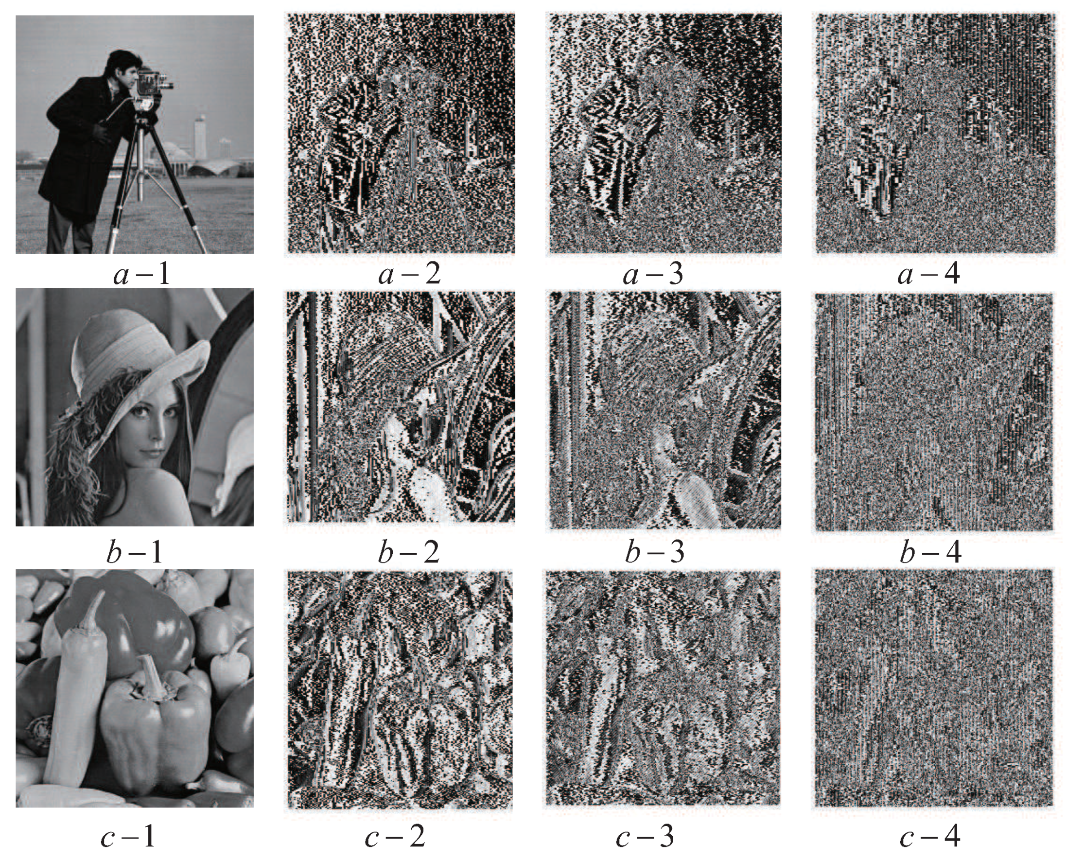
4. Results and Discussion

In this section, we use examples and experimental results to show the performance of the proposed scheme, and then compare the proposed scheme and previous TCSIS schemes.

Suppose the image is $O=(97,46,253,12,165,19,247,251,214,142,191,180,210,172,152)$. We construct a proposed $(3\leftrightarrow 5,7)$ TCSIS scheme for this image. Our proposed scheme is based on the computation of a $GF\left(P\right)$: $P=251$ and $P=2^8$ are adopted in our examples. When using $P=251$, all pixels that larger than 250 are transformed to 250 instead, and the computation is over $mod\left(251\right)$; therefore, the reconstructed image is of lower quality than the original image. When using $P=2^8$, no distortion would be caused from reconstructed image, but each pixel would need to be transferred into a polynomial, and the computation would be over $mod(x^8+x^4+x^3+x+1)$, which is much more complicated than the computation in $mod\left(251\right)$.

Example 1.

Proposed $(3\leftrightarrow 5,7)$ TCSIS on O over $GF\left(251\right)$.

First the original image O is transformed into image $O^{{}^{\prime }}$, where the pixels larger than 250 are transformed to 250. Then we get

$$O^{{}^{\prime }}=(97,46,250,12,165,19,247,250,214,142,191,180,210,172,152).$$

Next, a bivariate $F(x,y)$ with degree 2 on x and degree 4 on y is constructed based on $O^{{}^{\prime }}$.

$$F(x,y)=\left\{\begin{array}{c}97+46y+250y^2+12y^3+165y^4,\hfill \\ 19x+247xy+250x{y}^2+214x{y}^3+142x{y}^4,\hfill \\ 191x^2+180x^{2}y+210x^2{y}^2+172x^2{y}^3+152x^2{y}^4\hfill \end{array}\right.$$

(8)

Then the dealer computes $f_i\left(y\right)=F(i,y),g_i\left(x\right)=F(x,i),i=1,2,\dots ,7$ over $GF\left(251\right)$. The initial shadow ${\mathcal{S}}_i=(f_i\left(y\right),g_i\left(x\right))$ is sent to each participant $P_i,i=1,2,\dots ,7$ confidentially. The initial shadows ${\mathcal{S}}_1,{\mathcal{S}}_2,\dots ,{\mathcal{S}}_7$ are listed in Equation (9).

$$\left\{\begin{array}{c}{\mathcal{S}}_1:f_1\left(y\right)=56+222y+208y^2+147y^3+208y^4,g_1\left(x\right)=68+119x+152x^2\hfill \\ {\mathcal{S}}_2:f_2\left(y\right)=146+5y+84y^2+124y^3+53y^4,g_2\left(x\right)=160+226x+179x^2\hfill \\ {\mathcal{S}}_3:f_3\left(y\right)=116+148y+129y^2+194y^3+202y^4,g_3\left(x\right)=110+210x+250x^2\hfill \\ {\mathcal{S}}_4:f_4\left(y\right)=217+149y+92y^2+106y^3+153y^4,g_4\left(x\right)=101+86x+226x^2\hfill \\ {\mathcal{S}}_5:f_5\left(y\right)=198+8y+224y^2+111y^3+157y^4,g_5\left(x\right)=9+14x+102x^2\hfill \\ {\mathcal{S}}_6:f_6\left(y\right)=59+227y+23y^2+209y^3+214y^4,g_6\left(x\right)=156+48x+7x^2\hfill \\ {\mathcal{S}}_7:f_7\left(y\right)=51+53y+242y^2+149y^3+73y^4,g_7\left(x\right)=55+136x+204x^2\hfill \end{array}\right.$$

(9)

During image reconstruction, suppose the threshold is T, and $P_1,P_2,\dots ,P_T$ are involved.

• If $T=3$, $P_1,P_2,P_3$ publishes $S_i^3=f_i\left(y\right),i=1,2,3$, all coefficients in $F(x,y)$ can be computed using Lagrange interpolation according to Theorem 1. Then the image $O^{{}^{\prime }}$ can be reconstructed.
• If $T=4$, $P_1,P_2,P_3,P_4$ publish $S_i^4=g_i\left(x\right)\left|\right|f_i\left(e_1\right),i=1,2,3,4$. Here $e_1=8$. The interpolation polynomial on $f_i\left(e_1\right),i=1,2,3,4$ is $g_{e_1}\left(x\right)=F(x,e_1)=167+120x+86x^2$ for Example 1. Then, all coefficients in $F(x,y)$ can be computed using the Lagrange interpolation according to Theorem 3. Then the image $O^{{}^{\prime }}$ can be reconstructed.
• If $T=5$, $P_1-P_5$, publish $S_i^5=g_i\left(x\right),i=1,2,\dots ,5$. All coefficients in $F(x,y)$ can be computed using Lagrange interpolation according to Theorem 1. Then the image $O^{{}^{\prime }}$ can be reconstructed.

Example 2.

Proposed $(3\leftrightarrow 5,7)$ TCSIS on O over $GF\left(2^8\right)$.

A bivariate $F(x,y)$ with degree 2 on x and degree 4 on y is constructed based on O as follows.

$$F(x,y)=\left\{\begin{array}{c}97+46y+253y^2+12y^3+165y^4,\hfill \\ 19x+247xy+251x{y}^2+214x{y}^3+142x{y}^4,\hfill \\ 191x^2+180x^{2}y+210x^2{y}^2+172x^2{y}^3+152x^2{y}^4\hfill \end{array}\right.$$

(10)

Then the dealer computes $f_i\left(y\right)=F(i,y),g_i\left(x\right)=F(x,i),i=1,2,\dots ,7$ over $GF\left(2^8\right)$. The initial shadow ${\mathcal{S}}_i=(f_i\left(y\right),g_i\left(x\right))$ is sent to each participant $P_i,i=1,2,\dots ,7$ confidentially. The initial shadows ${\mathcal{S}}_1,{\mathcal{S}}_2,\dots ,{\mathcal{S}}_7$ are listed in Equation (11).

$$\left\{\begin{array}{c}{\mathcal{S}}_1:f_1\left(y\right)=205+109y+212y^2+118y^3+179y^4,g_1\left(x\right)=27+71x+237x^2\hfill \\ {\mathcal{S}}_2:f_2\left(y\right)=141+61y+117y^2+61y^3+244y^4,g_2\left(x\right)=58+245x+253x^2\hfill \\ {\mathcal{S}}_3:f_3\left(y\right)=33+126y+92y^2+71y^3+226y^4,g_3\left(x\right)=104+99x+106x^2\hfill \\ {\mathcal{S}}_4:f_4\left(y\right)=40+106y+179y^2+87y^3+232y^4,g_4\left(x\right)=168+119x+50x^2\hfill \\ {\mathcal{S}}_5:f_5\left(y\right)=132+41y+154y^2+45y^3+254y^4,g_5\left(x\right)=34+153x+200x^2\hfill \\ {\mathcal{S}}_6:f_6\left(y\right)=196+121y+59y^2+102y^3+185y^4,g_6\left(x\right)=168+219x+2x^2\hfill \\ {\mathcal{S}}_7:f_7\left(y\right)=104+58y+18y^2+28y^3+175y^4,g_7\left(x\right)=10+247x+61x^2\hfill \end{array}\right.$$

(11)

The reconstructions with different thresholds are similar to those in Example 1. Here we only emphasize that when the threshold is $T=4$, the participants can decide on $e_1=8$, and compute $g_{e_1}\left(x\right)=13+248x+98x^2$ in $GF\left(2^8\right)$, which is different from the $g_{e_1}\left(x\right)$ in Example 1.

The following Figure 3 shows the experimental results of the proposed $(5\leftrightarrow 7,9)$ over $GF\left(251\right)$, where the original image and initial shadows are included.

Next we give comparisons between the proposed TCSIS and the previous two TCSIS schemes [21,22] in detail. First we illustrate the information disclosure problem of the scheme in [22]. The initial shadows $S_i$ for each participant $P_i$ in [22] are generated from a $k-1$ degree polynomial $F_i^{*}\left(x\right)=F\left(x\right)+f_i\left(x\right)$, where $F\left(x\right)$ is of degree $k-1$, $f_i\left(x\right)$ is of degree $k^{{}^{\prime }}-1$, and $f_i\left(x\right)$ contains the pixels of secret image O. When the threshold is $k^{{}^{\prime }}$, each participant $P_i$ modifies its initial shadow by $S_i^{{}^{\prime }}=S_i-F\left(i\right)$; thus, the threshold of updated shadows is reduced to $k^{{}^{\prime }}$ from k. However, any $k^{{}^{\prime }}$ participants can recover a distortion image without updating their shadows, based on the homm. $S_i-S_j$ is generated from $F_i^{*}\left(x\right)-F_j^{*}\left(x\right)=f_i\left(x\right)-f_j\left(x\right)$. Since $f_i\left(x\right)-f_j\left(x\right)$ is of degree $k^{{}^{\prime }}-1$, any $k^{{}^{\prime }}$ participants can recover $f_i\left(x\right)-f_j\left(x\right)$. As a result, a distortion image can be recovered from the pixel information in $f_i\left(x\right)-f_j\left(x\right)$. The experimental results of information disclosure problem in [22] are shown in Figure 4.

The proposed TCSIS scheme generates initial shadows using bivariate polynomial $F(x,y)$, where image pixels are hidden in all coefficients in $F(x,y)$. Thus, the proposed scheme avoids the information disclosure problem in [22]. On the other hand, the the scheme in [22] only provides three potential thresholds $k^{{}^{\prime }},k,k^{{}^{″}}$ for low, medium, and high security levels, whereas our scheme can provide $h-k+1$ thresholds $k,k+1,k+2,\dots ,h$ to satisfy more complicated security requirements. The scheme in [21] can also provide more thresholds than the scheme in [22], but there are two weaknesses of the scheme in [21]. The dealer needs to publish certain information when changing a threshold; therefore, the participation of dealer in this process would not only reduce the efficiency of image reconstruction, but also risks information leakage from the communication between dealer and participants. Such problems also exist for the scheme presented in [22]. The other problem of the scheme in [21] is that the security is based on the security assumption of two-variable one-way functions; it is not unconditionally secure. In addition, the computation of one-way functions is much more complicated than the computation of polynomial interpolation. A comparison between the proposed scheme and the previous TCSIS schemes [21,22] is shown in

Table 1. A comparison of the three TCSIS schemes.

Schemes	Thresholds	Changing Threshold	Security Level	Main Computation	Shadow Size
Scheme [22]	$k^{{}^{\prime }},k,k^{{}^{″}}$	Dealer involves	Unconditional	Polynomial interpolation	$\frac{1}{k^{{}^{\prime }}}$
Scheme [21]	$T_1,T_2,\dots ,T_N$	Dealer involves	Conditional	One way function	$\frac{N}{T_N}$
Proposed scheme	$k,k+1,\dots ,h$	Without dealer	Unconditional	Polynomial interpolation	$\frac{k+h}{kh}$

.

5. Conclusions

In this paper, we constructed a $(k\leftrightarrow h,n)$ TCSIS scheme based on a bivariate polynomial that provides $h-k+1$ potential thresholds. During image reconstruction, participants can modify their initial shadows to adjust the threshold from $\{k,k+1,\dots ,h\}$. Compared with previous TCSIS schemes, our scheme has the following advantages:

• Our scheme provides more thresholds than the scheme in [22].
• Our scheme does not require the dealer’s involvement in changing the threshold, reducing its computational cost compared to the schemes in [21,22] and reducing the risk of information leakage.
• Our scheme does not adopt one-way functions; it achieves unconditional security.
• The computation is only based on polynomial interpolation, making it more efficient than the first scheme [21].

References

- Zhou, Z.L.; Wu, Q.J.; Yang, Y.M.; Sun, X.M. Region-level visual consistency verification for large-scale partial-duplicate image search. ACM Trans. Multimed. Comput. Commun. Appl. 2020, 16, 1–25. [Google Scholar] [CrossRef]
- Wang, C.C.; Kuo, W.C.; Huang, Y.C.; Wuu, L.C. A high capacity data hiding scheme based on re-adjusted GEMD. Multimed. Tools Appl. 2018, 77, 6327–6341. [Google Scholar] [CrossRef]
- Zhou, Z.L.; Mu, Y.; Wu, Q.J. Coverless image steganography using partial-duplicate image retrieval. Soft Comput. 2019, 23, 4927–4938. [Google Scholar] [CrossRef]
- Naor, M.; Shamir, A. Visual cryptography. Lect. Notes Comput. Sci. 1994, 950, 1–12. [Google Scholar]
- Wang, R.Z. Region incrementing visual cryptography. IEEE Signal Process. Lett. 2009, 16, 659–662. [Google Scholar] [CrossRef]
- Yang, C.N.; Shih, H.W.; Wu, C.C.; Harn, L. k out of n region incrementing scheme in visual cryptography. IEEE Trans. Circuits Syst. Video Technol. 2012, 22, 799–809. [Google Scholar] [CrossRef]
- Thien, C.C.; Lin, J.C. Secret image sharing. Comput. Graph. 2002, 26, 765–770. [Google Scholar] [CrossRef]
- Wang, R.Z.; Shyu, S.J. Scalable secret image sharing. Signal Process. Image Commun. 2007, 22, 363–373. [Google Scholar] [CrossRef]
- Liu, Y.X.; Yang, C.Y.; Yeh, P.H. Reducing shadow size in smooth scalable secret image sharing. Secur. Commun. Netw. 2014, 7, 2237–2244. [Google Scholar] [CrossRef]
- Wang, Z.H.; Di, Y.F.; Li, J.J.; Chang, C.C.; Liu, H. Progressive secret image sharing scheme using meaningful shadows. Secur. Commun. Netw. 2016, 9, 4075–4088. [Google Scholar] [CrossRef]
- Yan, X.H.; Wang, S.; Niu, X.M. Threshold progressive visual cryptography construction with unexpanded shares. Mutimedia Tools Appl. 2016, 75, 8657–8674. [Google Scholar] [CrossRef]
- Liu, Y.X.; Yang, C.N.; Wu, S.Y.; Chou, Y.S. Progressive (k, n) secret image sharing schemes based on Boolean operations and covering codes. Signal Process. Image Commun. 2018, 66, 77–86. [Google Scholar] [CrossRef]
- Liu, Y.X.; Yang, C.N. Scalable secret image sharing scheme with essential shadows. Signal Process. Image Commun. 2017, 58, 49–55. [Google Scholar] [CrossRef]
- Li, P.; Yang, C.N.; Wu, C.C.; Kong, Q.; Ma, Y. Essential secret image sharing scheme with different importance of shadows. J. Vis. Commun. Image Represent. 2013, 24, 1106–1114. [Google Scholar] [CrossRef]
- Yang, C.N.; Ouyang, J.F.; Harn, L. Steganography and authentication in image sharing without parity bits. Opt. Commun. 2012, 285, 1725–1735. [Google Scholar] [CrossRef]
- Ye, G.D.; Liu, M.; Wu, M.F. Double image encryption algorithm based on compressive sensing and elliptic curve. Alex. Eng. J. 2022, 61, 6785–6795. [Google Scholar] [CrossRef]
- Gong, L.H.; Qiu, K.D.; Deng, C.Z.; Zhou, N.R. An optical image compression and encryption scheme based on compressive sensing and RSA algorithm. Opt. Lasers Eng. 2019, 121, 169–180. [Google Scholar] [CrossRef]
- Zhang, Z.; Chee, Y.M.; Ling, S.; Liu, M.; Wang, H. Threshold changeable secret sharing schemes revisited. Theor. Comput. Sci. 2012, 418, 106–115. [Google Scholar] [CrossRef] [Green Version]
- Steinfeld, R.; Pieprzyk, J.; Wang, H.X. Lattice-based threshold-changeability for standard crt secret-sharing schemes. Finite Fields Their Appl. 2006, 12, 653–680. [Google Scholar] [CrossRef]
- Harn, L.; Hsu, C.F. Dynamic threshold secret reconstruction and its application to the threshold cryptography. Inf. Process. Lett. 2015, 115, 851–857. [Google Scholar] [CrossRef]
- Yuan, L.F.; Li, M.C.; Guo, C.; Hu, W.T.; Luo, X.J. Secret image sharing scheme with threshold changeable capability. Math. Probl. Eng. 2016, 2016, 9576074. [Google Scholar] [CrossRef] [Green Version]
- Liu, Y.X.; Yang, C.N.; Wu, C.M.; Sun, Q.D.; Bi, W. Threshold changeable secret image sharing scheme based on interpolation polynomial. Multimed. Tools Appl. 2019, 78, 18653–18667. [Google Scholar] [CrossRef]