Periodic Orbits of a Mosquito Suppression Model Based on Sterile Mosquitoes

Abstract

In this work, we investigate the existence and stability of periodic orbits of a mosquito population suppression model based on sterile mosquitoes. The model switches between two sub-equations as the actual number of sterile mosquitoes in the wild is assumed to take two constant values alternately. Employing the Poincaré map method, we show that the model has at most two T-periodic solutions when the release amount is not sufficient to eradicate the wild mosquitoes, and then obtain some sufficient conditions for the model to admit a unique or exactly two T-periodic solutions. In particular, we observe that the model displays bistability when it admits exactly two T-periodic solutions: the origin and the larger periodic solution are asymptotically stable, and the smaller periodic solution is unstable. Finally, we give two numerical examples to support our lemmas and theorems.

1. Introduction

Mosquito-borne diseases, such as dengue, malaria, Zika, yellow fever, West Nile fever, seriously imperil the health of people in tropical and sub-tropical areas. Recently, the rising global temperatures and uncontrolled urbanization greatly expand the threat range of such diseases [1,2,3]. The most direct approach to prevent and control these mosquito-borne diseases is to control the vector mosquitoes. Sterile Insect Technique (SIT) and Incompatible Insect Technique (IIT) are two promising and environment-friendly methods for controlling mosquitoes [4,5,6,7,8,9], which involve rearing massive number of sterile or Wolbachia-infected mosquitoes (these two kinds of mosquitoes are called sterile mosquitoes hereafter) in the laboratories or factories, then releasing them into the field to sterilize wild mosquitoes, and thus, the mosquito density can be asymptotically controlled.

Mathematical modeling has played an important role in the control and prevention of mosquito-borne diseases. One is to study the Wolbachia spread dynamics in mosquito populations aiming to study the possible invasion of Wolbachia in mosquito populations [10,11,12,13,14,15,16,17,18,19], and the other is to study the interactive dynamics of wild and sterile mosquitoes aiming to eliminate or control the wild mosquitoes below the risk of mosquito-borne disease outbreaks. Most early studies on the interactive dynamics mainly concentrate on models where the number of sterile mosquitoes was assumed to be an independent variable satisfying an independent dynamical equation, see, for example, [20,21,22,23,24], whereas recent investigations have proposed a motivation-attention modeling idea where the number of sterile mosquitoes is treated as a control function instead of an independent variable, since the fundamental and only role of sterile mosquitoes is to mate with wild mosquitoes to induce the infertility of wild females, see, for example, [25,26,27,28,29,30,31,32,33,34,35,36,37,38].

In [21], Li formulated the following model

$$\begin{array}{cc}\hfill \frac{dw}{dt}& =\frac{aw}{w+g}(1-\xi w)w-\mu w,\hfill \\ \hfill \frac{dg}{dt}& =B\left(w\right)-\mu g,\hfill \end{array}$$

(1)

to explore the interactive dynamics between wild and sterile mosquitoes. In this model, $w=w\left(t\right),g=g\left(t\right)$ are the numbers of wild and sterile mosquitoes at time t, respectively, a is the total number of offspring produced per wild mosquito, per unit of time, $\frac{w}{w+g}$ is the fraction of mates with wild mosquitoes, $\xi$ represents the carrying capacity of wild mosquitoes such that $1-\xi w$ characterizes the density-dependent survival probability, $\mu$ is the density-independent death rate coefficient of wild as well as sterile mosquitoes, and $B(·)$ is the rate of the releases of sterile mosquitoes. Under three different release strategies: constant releases ($B\left(w\right)=b$), proportional releases ($B\left(w\right)=bw$), and fractional releases ($B\left(w\right)=\frac{bw}{1+w}$), the author obtained the corresponding conditions for the existence and stabilities of positive equilibria.

Note that the sterile male mosquitoes are released to sterilize wild mosquitoes, along with the two facts: the lifespan of mosquitoes is short, and the sexual lifespan of those released sterile mosquitoes is much shorter than their longevity [39,40], it seems reasonable to ignore the death of those released sterile mosquitoes when they are sexually active and energetic. Moreover, the number of sterile mosquitoes that have been released into the field at time t is known in advance [9]. Hence, by regarding the number $g\left(t\right)$ of released sterile mosquitoes at time t as an arbitrarily given nonnegative continuous function, the authors in [28] omitted the second equation in (1), and studied the global dynamics of wild mosquitoes by the following model

$$\frac{dw}{dt}=\frac{aw}{w+g}(1-\xi w)w-\mu w.$$

(2)

This treatment greatly simplifies the model and makes the analysis mathematically more tractable.

In designing the release strategies of sterile mosquitoes, there are three important parameters: c, the release number in each batch; T, the waiting period between two adjacent releases; $\overline{T}$, the sexual lifespan of sterile mosquitoes. From the perspective of the relations between T and $\overline{T}$, there are three scenarios: $T>\overline{T},T=\overline{T}$ and $T<\overline{T}$. In [38], we studied the first case, and split Equation (2) into the following two sub-equations

$$\frac{dw}{dt}=\frac{a{w}^2(1-\xi w)}{w+c}-\mu w,t\in [iT,iT+\overline{T}),$$

(3)

and

$$\frac{dw}{dt}=a(1-\xi w)w-\mu w,t\in [iT+\overline{T},(i+1)T),$$

(4)

where $i=0,1,\dots$ We defined the first release amount threshold

$$g^{*}=\frac{{(a-\mu )}^2}{4a\mu \xi }.$$

(5)

Under the assumption of $c>g^{*}$, we further obtained the second release amount threshold $c^{*}$ and the waiting period threshold $T^{*}$ as follows

$$c^{*}=\frac{a-\mu }{\mu \xi },\mathrm{and}{T}^{*}=\frac{a}{a-\mu }\overline{T}.$$

We investigated Equations (3) and (4) for exploring the dynamical behaviors of wild mosquitoes under the interferences of released sterile mosquitoes.

However, rearing sterile mosquitoes needs huge economic input and puts the density of wild mosquitoes below a given value which is more realistic than eradicating them. Taking these facts into consideration, in this paper, we mainly discuss the dynamics of the model (3) and (4) under the release strategy of $c\le g^{*}$, which concentrates on reducing the number of wild mosquitoes with a lower cost than that in [38]. The remaining of the paper is structured as follows. In Section 2, we present some preparations, which mainly contain the introduction of the Poincaré map for determining the number of periodic solutions of the model (3) and (4), and some lemmas that are of vital importance to the proof of our main results. We give our main results in Section 3 and Section 4. In Section 5, we provide two numerical examples to verify our lemmas and theorems. Finally, some discussions on the current as well as future works are offered in Section 6.

2. Preliminaries

In this section, we give some lemmas, which provide a springboard to the proof of our main result.

Lemma 1

([38]). Assume that $c>g^{*}$ and $T>\overline{T}$. Then, the following conclusions are true.

$\left(\mathbf{1}\right)$

If $c\ge c^{*}$ and $T\le T^{*}$. Then, the origin, denoted by $E_0$, is globally asymptotically stable;

$\left(\mathbf{2}\right)$

If $T>T^{*}$ or $g^{*}<c<c^{*}$ and $T=T^{*}$. Then, the model (3) and (4) has a unique T-periodic solution, which is globally asymptotically stable;

$\left(\mathbf{3}\right)$

If $g^{*}<c<c^{*}$. Then, $E_0$ is locally asymptotically stable if and only if $T<T^{*}$.

We next give the definition of a solution of the model (3) and (4). A function $w\left(t\right)$ is said to be a solution of the model (3) and (4), if it satisfies both (3) and (4). Let $w\left(T^{-}\right)$ be the left limit of $w\left(T\right)$ with $w\left(T^{-}\right)=\underset{t\to T^{-}}{lim}w\left(t\right)$, and define

$$w\left(iT\right)=w\left({\left(iT\right)}^{-}\right),w(iT+\overline{T})=w({(iT+\overline{T})}^{-}),i=0,1,\dots$$

Then, $w\left(t\right)$ is a continuous and piecewise differentiable function defined on $[0,+\infty )$. Denote the solution of (3) and (4) with an initial value $w\left(0\right)=u>0$ by $w\left(t\right)=w(t;0,u)$. Then, $w\left(t\right)$ is a T-periodic solution of the model (3) and (4) provided that $w\left(T\right)=w(T;0,u)=u$. For convenience, we set

$$h\left(u\right):=w(T;0,u),\overline{h}\left(u\right):=w(\overline{T};0,u)$$

throughout this paper. Obviously, both $h\left(u\right)$ and $\overline{h}\left(u\right)$ are continuously differentiable functions in $u>0$.

As in [33], we define the following two sequences $h_n\left(u\right)$ and ${\overline{h}}_n\left(u\right)$ by

$$\left\{\begin{array}{c}{h}_n\left(u\right):=w(nT;0,u),\hfill \\ {\overline{h}}_n\left(u\right):=w(nT+\overline{T};0,u),\hfill \end{array}\right.n=0,1,\dots$$

The following lemma, which builds the relation between the signs of $h\left(u\right)-u$ and $h_n\left(u\right)-h_{n-1}\left(u\right),n=2,3,\dots$, plays an important role in judging the number of T-periodic solutions of the model (3) and (4).

Lemma 2

(Lemma 2.1 in [38]). For any given initial value u, the following conclusions hold.

$\left(1\right)$

Sequences $\left\{h_n\left(u\right)\right\}$ and $\left\{{\overline{h}}_n\left(u\right)\right\}$ are both strictly increasing if and only if $h\left(u\right)>u$.

$\left(2\right)$

$h_n\left(u\right)\equiv u,n=1,2,3,\dots$, if and only if $h\left(u\right)=u$. Hence, $w\left(t\right)=w(t;0,u)$ is a T-periodic solution of the model (3) and (4).

$\left(3\right)$

Sequences $\left\{h_n\left(u\right)\right\}$ and $\left\{{\overline{h}}_n\left(u\right)\right\}$ are both strictly decreasing if and only if $h\left(u\right)<u$.

Similar to Lemma 2.9 in [30], we give the following necessary and sufficient condition for $E_0$ to be asymptotically stable. The proof is also similar to that in [30] and we omit it here.

Lemma 3.

The origin $E_0$ is asymptotically stable if and only if there is ${\delta }_0>0$ such that

$$h\left(u\right)<u,\mathrm{for}u\in (0,{\delta }_0).$$

Lemma 2 tells us that the sign of $h^{\prime }\left(u\right)-1$ plays a key role in determining the number of T-periodic solutions of the model (3) and (4). To obtain this sign, we first solve Equation (3) for $t\in [0,\overline{T})$ to get the expression for $\overline{h}\left(u\right)$, and solve Equation (4) for $t\in [\overline{T},T)$ to get the relation between $\overline{h}\left(u\right)$ and $h\left(u\right)$. Then, we take the derivative of both sides of the above two expressions to get the expressions for ${\overline{h}}^{\prime }\left(u\right)$ and $h^{\prime }\left(u\right)$. We first consider Equation (4) as it is independent of c.

When $t\in [\overline{T},T)$, Equation (4) is

$$\frac{dw}{dt}=-a\xi w(w-A),$$

(6)

where $A=\frac{a-\mu }{a\xi }$. Further computations offer

$$d\left(ln\frac{w}{|A-w|}\right)=aA\xi dt.$$

(7)

Integrating (7) from $\overline{T}$ to T, we obtain

$$\frac{w\left(T\right)}{A-w\left(T\right)}=\frac{w\left(\overline{T}\right)}{A-w\left(\overline{T}\right)}{e}^{aA\xi (T-\overline{T})},$$

that is,

$$\frac{\overline{h}\left(u\right)}{A-\overline{h}\left(u\right)}=\frac{mh\left(u\right)}{A-h\left(u\right),}$$

(8)

where $m=e^{-aA\xi (T-\overline{T})}$.

When $t\in [0,\overline{T})$, we solve Equation (3) to obtain the expression for $\overline{h}\left(u\right)$. Since a solution may depends on the relations between c and $g^{*}$, we consider the following three possible cases.

Case (1):$0<c<g^{*}$. In this case, we can rewrite Equation (3) in the form

$$\frac{dw}{dt}=-\frac{a\xi w}{w+c}\left[{\left(w-\frac{A}{2}\right)}^2-\frac{\mu }{a\xi }(g^{*}-c)\right],$$

or, equivalently,

$$\frac{w+c}{w\left[{\left(w-\frac{A}{2}\right)}^2-\frac{\mu }{a\xi }(g^{*}-c)\right]}dw=-a\xi dt.$$

(9)

As $0<c<g^{*}$, we know that ${(w-\frac{A}{2})}^2-\frac{\mu }{a\xi }(g^{*}-c)=0$ has two real roots:

$$E_1\left(c\right)=\frac{A}{2}-\sqrt{\frac{\mu }{a\xi }(g^{*}-c)}\mathrm{and}{E}_2\left(c\right)=\frac{A}{2}+\sqrt{\frac{\mu }{a\xi }(g^{*}-c)}.$$

Then, we write (9) as

$$\frac{w+c}{w(w-E_1\left(c\right))(w-E_2\left(c\right))}dw=-a\xi dt.$$

(10)

By simple computations, we have

$$d\left\{ln\left[w^{{\alpha }_1}·|w-E_1{\left(c\right)|}^{{\beta }_1}·{|w-E_2\left(c\right)|}^{{\gamma }_1}\right]\right\}=-a\xi dt,$$

(11)

where

$${\alpha }_1=\frac{c}{E_1\left(c\right)E_2\left(c\right)},{\beta }_1=-\frac{c+E_1\left(c\right)}{E_1\left(c\right)(E_2\left(c\right)-E_1\left(c\right))},{\gamma }_1=\frac{c+E_2\left(c\right)}{E_2\left(c\right)(E_2\left(c\right)-E_1\left(c\right))}.$$

Integrating (11) from 0 to $\overline{T}$, along with the facts

$$w\left(0\right)=u,w\left(\overline{T}\right)=\overline{h}\left(u\right),$$

we obtain

$${\left(\frac{\overline{h}\left(u\right)}{u}\right)}^{{\alpha }_1}·{\left(\frac{\overline{h}\left(u\right)-E_1\left(c\right)}{u-E_1\left(c\right)}\right)}^{{\beta }_1}·{\left(\frac{\overline{h}\left(u\right)-E_2\left(c\right)}{u-E_2\left(c\right)}\right)}^{{\gamma }_1}=e^{-a\xi \overline{T}}.$$

(12)

Case (2): $c=g^{*}$. In this case, $E_1\left(c\right)=E_2\left(c\right)=\frac{A}{2}$. Set $E^{*}=\frac{A}{2}$. Then, Equation (3) is

$$\frac{dw}{dt}=-\frac{a\xi w}{w+g^{*}}{(w-E^{*})}^2.$$

(13)

Equation (13) is equivalent to

$$\frac{w+g^{*}}{w{(w-E^{*})}^2}dw=-a\xi dt,$$

which gives

$$\left(\frac{x}{w}+\frac{y}{w-E^{*}}+\frac{z}{{(w-E^{*})}^2}\right)dw=-a\xi dt,$$

(14)

where

$$x=\frac{g^{*}}{{\left(E^{*}\right)}^2},y=-\frac{g^{*}}{{\left(E^{*}\right)}^2},z=1+\frac{g^{*}}{E^{*}}.$$

We then transform (14) to

$$d\left\{ln\left[w^x·{|w-E^{*}|}^y·e^{-\frac{z}{w-E^{*}}}\right]\right\}=-a\xi dt,$$

which gives, by integrating from 0 to $\overline{T}$,

$${\overline{h}}^x\left(u\right)·{(\overline{h}\left(u\right)-E^{*})}^y·e^{-\frac{z}{\overline{h}\left(u\right)-E^{*}}}=u^x·{(u-E^{*})}^y·e^{-\frac{z}{u-E^{*}}}·e^{-a\xi \overline{T}}.$$

(15)

Case (3): $c>g^{*}$. In this case, we have from $\left(2.4\right)$ in [38]

$$\begin{array}{c}{\overline{h}}^{{\alpha }_2}\left(u\right)·{\left({\left(\overline{h}\left(u\right)-\frac{A}{2}\right)}^2+b^2\right)}^{\frac{{\beta }_2}{2}}·exp\left(\frac{{\gamma }_2}{b}{tan}^{-1}\left(\frac{\overline{h}\left(u\right)-\frac{A}{2}}{b}\right)\right)\hfill \\ \hfill \hspace{1em}\hspace{1em}\hspace{1em}\hspace{1em}\hspace{1em}\hspace{1em}=u^{{\alpha }_2}·{\left({\left(u-\frac{A}{2}\right)}^2+b^2\right)}^{\frac{{\beta }_2}{2}}·exp\left(\frac{{\gamma }_2}{b}{tan}^{-1}\left(\frac{u-\frac{A}{2}}{b}\right)\right)·e^{-a\xi \overline{T}},\end{array}$$

(16)

where

$${\alpha }_2=\frac{a\xi }{\mu },{\beta }_2=-\frac{a\xi }{\mu },{\gamma }_2=\frac{a+\mu }{2\mu },b=\sqrt{\frac{\mu }{a\xi }(c-g^{*})}.$$

Owing to the above preparations, we now give the following lemma, which manifests that the model (3) and (4) has no T-periodic solutions when $u\ge A$.

Lemma 4.

Assume that $u\ge A$. Then, $h\left(u\right)<u$.

Proof. 

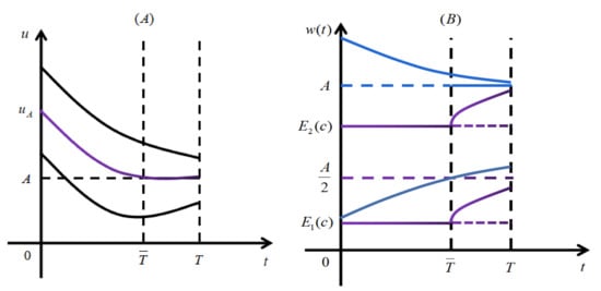
Due to the continuous dependence of the solutions on the initial data, the solution $w(t;0,u)$ is strictly increasing with respect to u, and it is strictly decreasing with respect to t for $t\in [0,\overline{T})$ when $u\ge A$. Then, there exists a unique $u_A>A$ such that $w(\overline{T};0,u_A)=A$, and $w(t;0,u_A)\equiv A$ when $t\in [\overline{T},T)$, which means that $h\left(u_A\right)=A<u_A$. Hence, solution $w(t;0,u)$ is strictly decreasing for $t\in [0,T]$ when $u>u_A$, as displayed in Figure 1A. Thus, when $u>u_A$, we have $h\left(u\right)=w(T;0,u)<u$, which shows that the lemma holds in this case. When $u\in [A,u_A)$, we have

$$h\left(u\right)=w(T;0,u)<w(T;0,u_A)=A\le u,$$

thus, the lemma also holds in this case. This completes the proof. □

Figure 1. (A): There exists a unique $u_A$ for the model (3) and (4) such that the solution $w\left(t\right)$ is strictly decreasing for $t\in [0,T]$ when $u>u_A$; (B): When $0<c<g^{*}$, the movement trend of the solution of the model (3) and (4) for $t\in [0,T]$ and $u\in [E_1\left(c\right),E_2\left(c\right)]$.

The following lemma tells us that the model (3) and (4) has no T-periodic solutions when $u\in [E_1\left(c\right),E_2\left(c\right)]$ with $c\in (0,g^{*}]$.

Lemma 5.

Assume that $0<c\le g^{*}$. Then, we have $h\left(u\right)>u$ for $u\in [E_1\left(c\right),E_2\left(c\right)]$.

Proof. 

If $c=g^{*}$, we have $E_1\left(c\right)=E_2\left(c\right)=E^{*}=\frac{A}{2}$, It follows from (6) and (13) that $h\left(E^{*}\right)>E^{*}$, which proves the lemma in this case.

If $c<g^{*}$, we have, according to (12),

$${\overline{h}}^{{\alpha }_1}\left(u\right)·{(\overline{h}\left(u\right)-E_1\left(c\right))}^{{\beta }_1}·{(\overline{h}\left(u\right)-E_2\left(c\right))}^{{\gamma }_1}=u^{{\alpha }_1}·{(u-E_1\left(c\right))}^{{\beta }_1}·{(u-E_2\left(c\right))}^{{\gamma }_1}·e^{-a\xi \overline{T}}.$$

(17)

Set

$$\kappa \left(u\right)=u^{{\alpha }_1}·{(u-E_1\left(c\right))}^{{\beta }_1}·{(u-E_2\left(c\right))}^{{\gamma }_1}.$$

(18)

Then, $\kappa \left(u\right)<0$, and (17) becomes $\kappa \left(\overline{h}\left(u\right)\right)=\kappa \left(u\right)e^{-a\xi \overline{T}}$, which shows that $\kappa \left(\overline{h}\left(u\right)\right)>\kappa \left(u\right)$. By taking the derivative on both sides of (18), we obtain

$${\kappa }^{\prime }\left(u\right)=\kappa \left(u\right)\frac{u+c}{u(u-E_1\left(c\right))(u-E_2\left(c\right))}>0,u\in (E_1\left(c\right),E_2\left(c\right)).$$

Hence, we obtain $\overline{h}\left(u\right)>u$. Moreover, from the fact $0<E_1\left(c\right)<E_2\left(c\right)<A$ (see the diagram depicted in Figure 1B), we see that $w(t;0,u)$ is strictly increasing for $t\in [\overline{T},T]$, and so $h\left(u\right)=w(T;0,u)>w(\overline{T},0,u)=\overline{h}\left(u\right)>u$. Obviously, when $u=E_1\left(c\right)$ or $u=E_2\left(c\right)$, we also have $h\left(u\right)>u$. The proof is completed. □

When $u\in (0,E_1\left(c\right))$, the following lemma implies that the model (3) and (4) has at most one T-periodic solution.

Lemma 6.

Assume that $0<c\le g^{*}$. Then, $h\left(u\right)-u=0$ has at most one positive root when $u\in (0,E_1\left(c\right))$.

Proof. 

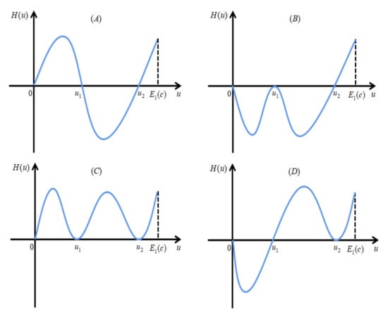
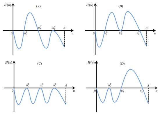
We divide the proof into two cases of $0<c<g^{*}$ and $c=g^{*}$. Define $H\left(u\right)=h\left(u\right)-u$. For the case when $0<c<g^{*}$, assume by contradiction that $H\left(u\right)=0$ has at least two positive real roots for $u\in (0,E_1\left(c\right))$, denote the largest two adjacent roots by $u_1$ and $u_2$, with $0<u_1<u_2<E_1\left(c\right)$. Note that we already have $H\left(E_1\left(c\right)\right)=h\left(E_1\left(c\right)\right)-E_1\left(c\right)>0$ from Lemma 5. Hence, we must have $H^{\prime }\left(u_2\right)\ge 0$. See Figure 2 for illustration.

Figure 2. Panels (A–D) are four possible cases when $H\left(u\right)=0$ has exactly two positive real roots for $u\in (0,E_1\left(c\right))$.

For convenience, we let $E_i\left(c\right)=E_i$ with $i=1,2$ hereafter. From (12), we have

$${\overline{h}}^{{\alpha }_1}\left(u\right)·{(E_1-\overline{h}\left(u\right))}^{{\beta }_1}·{(E_2-\overline{h}\left(u\right))}^{{\gamma }_1}=u^{{\alpha }_1}·{(E_1-u)}^{{\beta }_1}·{(E_2-u)}^{{\gamma }_1}·e^{-a\xi \overline{T}}.$$

(19)

Calculating the derivative on both sides of (19), we obtain

$$\begin{array}{c}{\overline{h}}^{{\alpha }_1}\left(u\right)·{(E_1-\overline{h}\left(u\right))}^{{\beta }_1}·{(E_2-\overline{h}\left(u\right))}^{{\gamma }_1}·\frac{\overline{h}\left(u\right)+c}{\overline{h}\left(u\right)(\overline{h}\left(u\right)-E_1)(\overline{h}\left(u\right)-E_2)}·{\overline{h}}^{\prime }\left(u\right)\hfill \\ \hfill =u^{{\alpha }_1}·{(E_1-u)}^{{\beta }_1}·{(E_2-u)}^{{\gamma }_1}·e^{-a\xi \overline{T}}·\frac{u+c}{u(u-E_1)(u-E_2)},\end{array}$$

which, combining with (19), gives

$${\overline{h}}^{\prime }\left(u\right)=\frac{\overline{h}\left(u\right)(\overline{h}\left(u\right)-E_1)(\overline{h}\left(u\right)-E_2)(u+c)}{u(u-E_1)(u-E_2)(\overline{h}\left(u\right)+c)}.$$

(20)

From (8), we get

$$h\left(u\right)=\frac{A\overline{h}\left(u\right)}{mA+(1-m)\overline{h}\left(u\right)}\mathrm{or}\overline{h}\left(u\right)=\frac{mAh\left(u\right)}{A-(1-m)h\left(u\right)},$$

(21)

which indicates

$$\begin{array}{ccc}\hfill & A-\overline{h}\left(u\right)=\frac{A(A-h(u\left)\right)}{A-(1-m)h\left(u\right)},\hfill & \hfill \overline{h}\left(u\right)-E_1=\frac{-A{E}_1+(m{E}_2+E_1)h\left(u\right)}{A-(1-m)h\left(u\right)},\\ \hfill & \overline{h}\left(u\right)-E_2=\frac{-A{E}_2+(m{E}_1+E_2)h\left(u\right)}{A-(1-m)h\left(u\right)},\hfill & \hfill \overline{h}\left(u\right)+c=\frac{cA+\left(mA-\left(1-m\right)c\right)h\left(u\right)}{A-(1-m)h\left(u\right)}.\end{array}$$

(22)

Moreover, by taking the derivative on both sides of (21), we arrive at

$${\overline{h}}^{\prime }\left(u\right)=\frac{m{A}^2{h}^{\prime }\left(u\right)}{{(A-(1-m)h\left(u\right))}^2},$$

or, equivalently,

$$\frac{{\overline{h}}^{\prime }\left(u\right)}{\overline{h}\left(u\right)(A-\overline{h}\left(u\right))}=\frac{h^{\prime }\left(u\right)}{h\left(u\right)(A-h(u\left)\right)},$$

which yields, along with (20),

$$h^{\prime }\left(u\right)=\frac{h\left(u\right)(A-h\left(u\right))(\overline{h}\left(u\right)-E_1)(\overline{h}\left(u\right)-E_2)(u+c)}{u(A-\overline{h}\left(u\right))(u-E_1)(u-E_2)(\overline{h}\left(u\right)+c)}.$$

(23)

Substituting (22) into (23), we obtain

$$h^{\prime }\left(u\right)=\frac{h\left(u\right)[A{E}_1-(m{E}_2+E_1)h\left(u\right)][A{E}_2-(m{E}_1+E_2)h\left(u\right)](u+c)}{Au(E_1-u)(E_2-u)\{cA+[mA-(1-m)c]h\left(u\right)\}}.$$

(24)

From the two facts that $h\left(u_2\right)=u_2$ and $h^{\prime }\left(u_2\right)\ge 1$, we get

$$h^{\prime }\left(u_2\right)=\frac{[A{E}_1-(m{E}_2+E_1)u_2][A{E}_2-(m{E}_1+E_2)u_2](u_2+c)}{A(E_1-u_2)(E_2-u_2)\{cA+[mA-(1-m)c]u_2\}}\ge 1,$$

(25)

which, along with $E_1+E_2=A$, gives

$$B{u}_2^2+C{u}_2+D\ge 0,$$

(26)

where the three coefficients $B,C,D$ are defined as

$$\begin{array}{cc}\hfill B& =(1-m)E_1{E}_2+cA,\hfill \\ \hfill C& =((1-m)c-2A)E_1{E}_2-2c{A}^2,\hfill \\ \hfill D& =A((A-c)E_1{E}_2+c{A}^2).\hfill \end{array}$$

(27)

Define

$$\chi \left(u\right)=B{u}^2+Cu+D.$$

(28)

Then, (26) becomes $\chi \left(u_2\right)\ge 0$. For the relation between $h^{\prime }\left(u_1\right)$ and 1, we need to consider two cases: (I) $h^{\prime }\left(u_1\right)\le 1$ (see panels (A), (B) and (C) in Figure 2 for illustration), and (II) $h^{\prime }\left(u_1\right)>1$ (see panel (D) in Figure 2 for illustration). Next, we prove that both cases (I) and (II) are impossible.

For case (I), similar to the relation between the two signs of $h^{\prime }\left(u_2\right)-1$ and $\chi \left(u_2\right)$, we have $\chi \left(u_1\right)\le 0$. Furthermore, we have the following observations:

$$\begin{array}{cc}\hfill & \chi \left(0\right)=D>0,{\chi }^{\prime }\left(0\right)=C=-((1+m)c+2A)E_1{E}_2+2c(E_1{E}_2-A^2)<0,\hfill \\ \hfill & \chi \left(E_1\right)=B{E}_1^2+C{E}_1+D=(E_1+c)\left[(1-m)E_1^2{E}_2+A{E}_2(E_2-E_1)\right]>0,\hfill \\ \hfill & {\chi }^{\prime }\left(E_1\right)=2B{E}_1+C=-(2m{E}_1+(1+m)c)E_1{E}_2-2E_2^2(E_1+c)<0.\hfill \end{array}$$

(29)

Hence, we get

$$\chi \left(u\right)>0,u\in (0,E_1).$$

(30)

Thus, $\chi \left(u_1\right)>0$, which contradicts $\chi \left(u_1\right)\le 0$.

Furthermore, if case (II) holds, then we gain $h^{\prime }\left(u_2\right)=1$, or, equivalently, $\chi \left(u_2\right)=0$, which also contradicts (30). The proof for the case of $0<c<g^{*}$ is completed.

For the case when $c=g^{*}$, using similar arguments that led to (25), we have

$$h^{\prime }\left(u_2\right)=\frac{{\{mA{u}_2-E^{*}[A-(1-m)u_2]\}}^2(u_2+g^{*})}{A{(u_2-E^{*})}^2\{mA{u}_2+g^{*}[A-(1-m)u_2]\}}\ge 1,$$

(31)

the remaining proof is similar to that of case $0<c<g^{*}$ and is omitted. We complete the proof. □

The following lemma tells us that the model (3) and (4) has a unique T-periodic solution when $u\in (E_2,A)$.

Lemma 7.

Assume that $0<c\le g^{*}$. Then, $h\left(u\right)-u=0$ has exactly one positive real root in $(E_2,A)$.

Proof. 

We first consider the case $0<c<g^{*}$. From Lemmas 4 and 5, we obtain

$$h\left(E_2\right)>E_2\mathrm{and}h\left(A\right)<A.$$

(32)

Then, there exists $\widehat{u}\in (E_2,A)$ such that $H\left(\widehat{u}\right)=h\left(\widehat{u}\right)-\widehat{u}=0$. Next, we prove that $\widehat{u}$ is the unique positive real root of $H\left(u\right)=0$ for $u\in (E_2,A)$.

Assume by contradiction that $H\left(u\right)=0$ has at least two positive real roots for $u\in (E_2,A)$, and the smallest and largest are denoted by ${\overline{u}}_1$ and ${\overline{u}}_2$, respectively. Hence, (32) implies that

$$H\left(u\right)>0,u\in (E_2,{\overline{u}}_1),\mathrm{and}H\left(u\right)<0,u\in ({\overline{u}}_2,A).$$

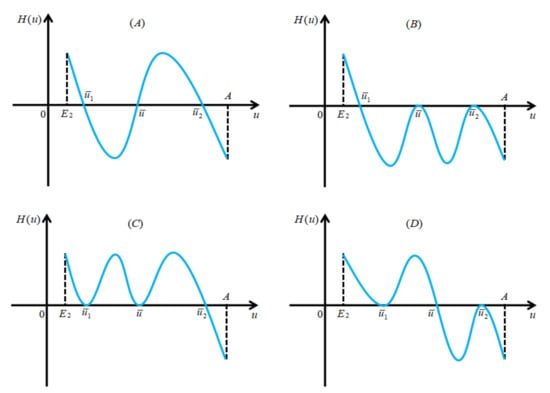
Thus, we obtain $H^{\prime }\left({\overline{u}}_i\right)\le 0,i=1,2$. However, from the continuous differentiability of $H\left(u\right)$, we know that there exists $\overline{u}\in [{\overline{u}}_1,{\overline{u}}_2]$ such that $H\left(\overline{u}\right)=0$. We consider two cases: (I) $H^{\prime }\left(\overline{u}\right)\ge 0$ (see panels (A–C) in Figure 3 for illustration) and (II) $H^{\prime }\left(\overline{u}\right)<0$ (see Figure 3D for illustration) to discuss the signs of $H^{\prime }\left(\overline{u}\right)$.

Figure 3. Schematic illustrations of the signs of $H^{\prime }\left(\overline{u}\right)$. Panels (A–C) manifest $H^{\prime }\left(\overline{u}\right)\ge 0$, and panel (D) represents $H^{\prime }\left(\overline{u}\right)<0$.

For case (I), we have

$$h\left({\overline{u}}_i\right)={\overline{u}}_i,h^{\prime }\left({\overline{u}}_i\right)\le 1,i=1,2,\mathrm{and}h\left(\overline{u}\right)=\overline{u},h^{\prime }\left(\overline{u}\right)\ge 1,$$

which yields

$$\chi \left({\overline{u}}_1\right)\le 0,\chi \left({\overline{u}}_2\right)\le 0,\mathrm{and}\chi \left(\overline{u}\right)\ge 0,$$

where $\chi \left(u\right)$ is defined in (28). To complete the proof, we consider two cases of $\chi \left(\overline{u}\right)>0$ and $\chi \left(\overline{u}\right)=0$ separately. Since we already know that $B>0$ and $\chi \left(u\right)$ is a quadratic polynomial, the first case does not hold. Now, we focus on the latter one. There exist two sub-cases for $\chi \left(\overline{u}\right)=0$, that is, (a)$\overline{u}\in ({\overline{u}}_1,{\overline{u}}_2)$; and (b)$\overline{u}={\overline{u}}_1\mathrm{or}\overline{u}={\overline{u}}_2$.

By similar arguments used in the situation $\chi \left(\overline{u}\right)>0$, we can show that sub-case (a) does not hold. For sub-case (b), we first use the perturbation method to discuss the case of $\overline{u}={\overline{u}}_1$.

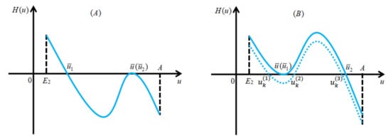
To this end, let $k>1$ be small enough such that $h\left(u\right)-ku=0$ has exactly three positive real roots, denoted by $u_k^{\left(i\right)},i=1,2,3$, satisfying

$$0<u_k^{\left(1\right)}<{\overline{u}}_1<u_k^{\left(2\right)}<u_k^{\left(3\right)}<{\overline{u}}_2,$$

and

$$h^{\prime }\left(u_k^{\left(1\right)}\right)\le k,h^{\prime }\left(u_k^{\left(2\right)}\right)\ge k,h^{\prime }\left(u_k^{\left(3\right)}\right)\le k.$$

(33)

See Figure 4B for illustration.

Figure 4. Panel (A) indicates the case that equation $h\left(u\right)-ku=0$ has two positive real roots; panel (B) shows that the equation may have exactly three positive real roots by small perturbation based on the solid curve in panel (B).

Substituting $h\left(u_k^{\left(i\right)}\right)=k{u}_k^{\left(i\right)}(i=1,2,3)$ into (24), we have

$$h^{\prime }\left(u_k^{\left(i\right)}\right)=\frac{k\left[(m{E}_2+E_1)k{u}_k^{\left(i\right)}-A{E}_1\right]\left[(m{E}_1+E_2)k{u}_k^{\left(i\right)}-A{E}_2\right]\left(u_k^{\left(i\right)}+c\right)}{A\left(u_k^{\left(i\right)}-E_1\right)\left(u_k^{\left(i\right)}-E_2\right)\left\{cA+[mA-(1-m)c]k{u}_k^{\left(i\right)}\right\}},i=1,2,3,$$

which yields, by (33),

$$\begin{array}{c}\hfill B\left(k\right){\left(u_k^{\left(1\right)}\right)}^2+C\left(k\right)u_k^{\left(1\right)}+D\left(k\right)\le 0,\\ \hfill B\left(k\right){\left(u_k^{\left(2\right)}\right)}^2+C\left(k\right)u_k^{\left(2\right)}+D\left(k\right)\ge 0,\\ \hfill B\left(k\right){\left(u_k^{\left(3\right)}\right)}^2+C\left(k\right)u_k^{\left(3\right)}+D\left(k\right)\le 0,\end{array}$$

(34)

with $B\left(k\right),C\left(k\right),D\left(k\right)$ being defined as follows:

$$\begin{array}{cc}\hfill B\left(k\right)& =k^2{(1-m)}^2{E}_1{E}_2+km(k-1)A^2+kc(1-m)A,\hfill \\ \hfill C\left(k\right)& =k(1-m)(kc(1-m)-2A)E_1{E}_2+c(1+k)(km-1)A^2,\hfill \\ \hfill D\left(k\right)& =(1-km)(cA+E_1{E}_2)A^2-ck(1-m)A{E}_1{E}_2.\hfill \end{array}$$

Hence, we have $B\left(k\right)>0$, from the fact $m<1<k$.

Set

$${\chi }_k\left(u\right)=B\left(k\right)u^2+C\left(k\right)u+D\left(k\right).$$

Then, we have, from (34),

$${\chi }_k\left(u_k^{\left(1\right)}\right)\le 0,{\chi }_k\left(u_k^{\left(2\right)}\right)\ge 0,\mathrm{and}{\chi }_k\left(u_k^{\left(3\right)}\right)\le 0,$$

which contradicts $B\left(k\right)>0$ and ${\chi }_k\left(u\right)$ is a quadratic polynomial. This proves that $\overline{u}={\overline{u}}_1$ is impossible.

Moreover, if $\overline{u}={\overline{u}}_2$, then $H^{\prime }\left(\overline{u}\right)=0$, and hence $\chi \left(\overline{u}\right)=0$. However, we find that

$$\chi \left(A\right)=B{A}^2+CA+D=-m{E}_1{E}_{2}A(A+c)<0,$$

which derives a contradiction, since ${\overline{u}}_1<\overline{u}<A$ and $B>0$ and $\chi \left(u\right)$ is a quadratic polynomial. Thus, sub-case $\left(b\right)$ is also impossible, and hence case (I) is impossible.

For case (II), we obtain

$$H^{\prime }\left({\overline{u}}_i\right)=0,i=1,2,\mathrm{and}{H}^{\prime }\left(\overline{u}\right)<0,$$

which leads to $\chi \left(A\right)>0$, a contradiction to $\chi \left(A\right)<0$, and hence case (II) is also impossible, which manifests that the lemma holds for the case when $0<c<g^{*}$.

For the case $c=g^{*}$, by using similar arguments to those in the proof of the case $0<c<g^{*}$, we can prove the lemma also holds in this case. The proof is thus completed. □

3. At Most Two Periodic Solutions

In this section, we give the main theorem, whose proof involves Lemmas 1–7, and tackles three different cases under the release strategy of $T>\overline{T}$.

Theorem 1.

Assume that $T>\overline{T}$. Then, the model (3) and (4) admits at most two T-periodic solutions.

Proof. 

We divide the proof into the following three cases:

$$\left(\mathrm{i}\right)0<c\le g^{*};\left(\mathrm{ii}\right)g^{*}<c<c^{*};\left(\mathrm{iii}\right)c\ge c^{*}.$$

For case (i), Lemmas 4–7 tell us that the model (3) and (4) has no T-periodic solutions when $u\in [E_1,E_2]\cup [A,+\infty )$, exactly one T-periodic solution when $u\in (E_2,A)$, at most one T-periodic solution when $u\in (0,E_1)$; these facts manifest that the model (3) and (4) has at most two T-periodic solutions in this case.

For case (ii), from Lemma 1(2), we know that the model (3) and (4) has a unique T-periodic solution for the case when $T\ge T^{*}$. Hence, we only need to consider the case of $T<T^{*}$.

Assume by contradiction that the model (3) and (4) has at least three T-periodic solutions. Let $w_1\left(t\right)=w(t;0,u_1^0)$ and $w_2\left(t\right)=w(t;0,u_2^0)$ be the two periodic solutions with the smallest and largest initial value, respectively. From Lemma 4, we obtain that $u_i^0\in (0,A),i=1,2$. From Lemma 1(3), we know that $E_0$ is locally asymptotically stable, which gives

$$h\left(u\right)<u,u\in (0,u_1^0)\cup (u_2^0,A),\mathrm{and}{h}^{\prime }\left(u_1^0\right)\ge 1,h^{\prime }\left(u_2^0\right)\le 1.$$

If the model (3) and (4) has exactly three T-periodic solutions, we denote the third T-periodic solution by $w_3\left(t\right)=w(t;0,u_3^0)$. For the relations between $h^{\prime }\left(u_3^0\right)$ and 1, as shown in Figure 5, we need to consider two possible cases: $h^{\prime }\left(u_3^0\right)<1$ and $h^{\prime }\left(u_3^0\right)\ge 1$.

Figure 5. Set $g^{*}<c<c^{*}$. Panels (A–D) present four possible situations when the model (3) and (4) has exactly three T-periodic solutions.

Here, we only consider the case of $h^{\prime }\left(u_3^0\right)\ge 1$, as the analysis for the case of $h^{\prime }\left(u_3^0\right)<1$ is similar and is omitted. There exists $u_4^0\in [u_1^0,u_3^0]$ such that $h\left(u_4^0\right)=u_4^0$ and $h^{\prime }\left(u_4^0\right)\le 1$. Let

$$\mathsf{\Phi }\left(u\right)=u^{{\alpha }_2}{\left({\left(u-\frac{A}{2}\right)}^2+b^2\right)}^{\frac{{\beta }_2}{2}}exp\left\{\frac{{\gamma }_2}{b}{tan}^{-1}\left(\frac{u-\frac{A}{2}}{b}\right)\right\}.$$

(35)

Then, we have

$${\mathsf{\Phi }}^{\prime }\left(u\right)=\left(\frac{{\alpha }_2}{u}+\frac{{\beta }_2\left(u-\frac{A}{2}\right)+{\gamma }_2}{{\left(u-\frac{A}{2}\right)}^2+b^2}\right)\mathsf{\Phi }\left(u\right)=\frac{u+c}{u\left({\left(u-\frac{A}{2}\right)}^2+b^2\right)}\mathsf{\Phi }\left(u\right).$$

(36)

By (35), (16) becomes

$$\mathsf{\Phi }\left(\overline{h}\left(u\right)\right)=\mathsf{\Phi }\left(u\right)e^{-a\xi \overline{T}},$$

(37)

which gives, by taking the derivative on both sides,

$${\mathsf{\Phi }}^{\prime }\left(\overline{h}\left(u\right)\right){\overline{h}}^{\prime }\left(u\right)={\mathsf{\Phi }}^{\prime }\left(u\right)e^{-a\xi \overline{T}},$$

(38)

substituting (36) and (37) into (38), we obtain

$${\overline{h}}^{\prime }\left(u\right)=\frac{\overline{h}\left(u\right)\left({\left(\overline{h}\left(u\right)-\frac{A}{2}\right)}^2+b^2\right)(u+c)}{u\left({\left(u-\frac{A}{2}\right)}^2+b^2\right)(\overline{h}\left(u\right)+c)}.$$

(39)

Taking the derivative on both sides of (8), we get

$$\frac{{\overline{h}}^{\prime }\left(u\right)}{{(A-\overline{h}\left(u\right))}^2}=\frac{m{h}^{\prime }\left(u\right)}{{(A-h\left(u\right))}^2}.$$

(40)

Substituting (8) and (39) into (40), we reach

$$h^{\prime }\left(u\right)=\frac{h\left(u\right)\left\{\frac{A^2}{4}{[A-(1+m)h\left(u\right)]}^2+b^2{[A-(1-m)h\left(u\right)]}^2\right\}(u+c)}{Au\left({\left(u-\frac{A}{2}\right)}^2+b^2\right)\left\{cA+[mA-(1-m\left)c\right]h\left(u\right)\right\}}.$$

Then, we have

$$\begin{array}{c}\hfill h^{\prime }\left(u_1^0\right)=\frac{\left\{\frac{A^2}{4}{[A-(1+m)u_1^0]}^2+b^2{[A-(1-m)u_1^0]}^2\right\}(u_1^0+c)}{A\left({\left(u_1^0-\frac{A}{2}\right)}^2+b^2\right)\left\{cA+[mA-(1-m)c]u_1^0\right\}}\ge 1,\\ \hfill h^{\prime }\left(u_2^0\right)=\frac{\left\{\frac{A^2}{4}{[A-(1+m)u_2^0]}^2+b^2{[A-(1-m)u_2^0]}^2\right\}(u_2^0+c)}{A\left({\left(u_2^0-\frac{A}{2}\right)}^2+b^2\right)\left\{cA+[mA-(1-m)c]u_2^0\right\}}\le 1,\\ \hfill h^{\prime }\left(u_3^0\right)=\frac{\left\{\frac{A^2}{4}{[A-(1+m)u_3^0]}^2+b^2{[A-(1-m)u_3^0]}^2\right\}(u_3^0+c)}{A\left({\left(u_3^0-\frac{A}{2}\right)}^2+b^2\right)\left\{cA+[mA-(1-m)c]u_3^0\right\}}\ge 1,\end{array}$$

(41)

and

$$h^{\prime }\left(u_4^0\right)=\frac{\left\{\frac{A^2}{4}{[A-(1+m)u_4^0]}^2+b^2{[A-(1-m)u_4^0]}^2\right\}(u_4^0+c)}{A\left({\left(u_4^0-\frac{A}{2}\right)}^2+b^2\right)\left\{cA+[mA-(1-m)c]u_4^0\right\}}\le 1.$$

(42)

Define

$$\mathsf{\Omega }\left(u\right)=B_0{u}^2+C_{0}u+D_0,$$

where

$$B_0=\frac{a-m\mu }{a\xi },C_0=\frac{(1-m)c\mu \xi -2(a-\mu )}{a{\xi }^2},D_0=-\frac{\mu (c-c^{*})}{a\xi }A.$$

Then, (41) and (42) imply

$$\mathsf{\Omega }\left(u_1^0\right)\ge 0,\mathsf{\Omega }\left(u_4^0\right)\le 0,\mathsf{\Omega }\left(u_3^0\right)\ge 0,\mathsf{\Omega }\left(u_2^0\right)\le 0.$$

(43)

Note that $B_0>0$ and $\mathsf{\Omega }\left(u\right)$ is a quadratic polynomial and $u_1^0\le u_4^0\le u_3^0\le u_2^0$, which violate (43). The proof is completed in this case.

For case (iii), Lemma 1(1) and Lemma 1(2) manifest that the model (3) and (4) has at most one T-periodic solution. We complete the proof. □

4. A Unique and Exact Two Periodic Solutions

Lemmas 4–7 imply that the model (3) and (4) has at least one and at most two T-periodic solutions when $0<c\le g^{*}$. In this section, we give the corresponding sufficient and necessary conditions for the model (3) and (4) to admit a unique or exactly two T-periodic solutions, which shows that the wild mosquitoes can be eradicated only if their initial population size is less than a given value.

Theorem 2.

Assume that $0<c\le g^{*}$. Then, the following two conclusions hold.

$\left(1\right)$

Model (3) and (4) has a unique globally asymptotically stable T-periodic solution, if and only if $E_0$ is unstable;

$\left(2\right)$

Model (3) and (4) has exactly two T-periodic solutions if and only if $E_0$ is locally asymptotically stable. For the two T-periodic solutions, the one with a larger initial value is asymptotically stable, and the other is unstable.

Proof. 

Lemma 7 tells us that the model (3) and (4) has a unique T-periodic solution when $u\in (E_2,A)$. Denote the unique T-periodic solution by $\widehat{w}\left(t\right)=w(t;0,\widehat{u})$. Then, we have

$$h\left(u\right)>u,u\in (E_1,\widehat{u}),\mathrm{and}h\left(u\right)<u,u\in (\widehat{u},+\infty ).$$

(44)

(1) Assume that $\widehat{w}\left(t\right)$ is globally asymptotically stable. Then, obviously, $E_0$ is unstable. Furthermore, assume $E_0$ is unstable. Then, there exists $\overline{\delta }>0$ such that $h\left(u\right)>u$ holds for all $u\in (0,\overline{\delta })$, which gives, by Lemma 6 and (44),

$$h\left(u\right)>u,u\in (0,E_1].$$

This, along with (44), we get

$$h\left(u\right)>u,u\in (0,\widehat{u}),\mathrm{and}h\left(u\right)<u,u\in (\widehat{u},+\infty ).$$

The proof of the global asymptotic stability of $\widehat{w}\left(t\right)$ is similar to that of Theorem 3.4 in [38] and is omitted.

(2) From Lemmas 4–7, we find that “model (3) and (4) has exactly two T-periodic solutions” is equivalent to “$h\left(u\right)-u=0$ has exactly one positive real root in $(0,E_1)$”. We first show that $E_0$ is asymptotically stable provided that $h\left(u\right)-u=0$ has exactly one positive real root in $(0,E_1)$. Let $u^{*}\in (0,E_1)$ denote this root. From (44), we reach

$$h\left(u\right)>u,u\in (u^{*},\widehat{u}),\mathrm{and}h\left(u\right)<u,u\in (\widehat{u},+\infty ).$$

(45)

Next, we prove

$$h\left(u\right)<u,u\in (0,u^{*}).$$

(46)

Assume by contradiction that (46) is not true. Note that $h\left(u\right)-u=0$ has no positive real roots in $(0,u^{*})$, then $h\left(u\right)>u$ holds for all $u\in (0,u^{*})$. This, along with (45) and $h\left(u^{*}\right)=u^{*}$, indicates $h^{\prime }\left(u^{*}\right)=1$. If $c\in (0,g^{*})$, then we get, from (24),

$$h^{\prime }\left(u^{*}\right)=\frac{[A{E}_1-(m{E}_2+E_1)u^{*}][A{E}_2-(m{E}_1+E_2)u^{*}](u^{*}+c)}{A(E_1-u^{*})(E_2-u^{*})\{cA+[mA-(1-m)c]u^{*}\}}=1,$$

which yields

$$\chi \left(u^{*}\right)=B{\left(u^{*}\right)}^2+C{u}^{*}+D=0,$$

where $B,C,D$ are defined in (27). From (29), we have $\chi \left(0\right)>0,{\chi }^{\prime }\left(0\right)<0,\chi \left(E_1\right)>0,{\chi }^{\prime }\left(E_1\right)<0$, which indicates that $\chi \left(u\right)>0$ holds for all $u\in (0,E_1)$, and this contradicts $u^{*}\in (0,E_1)$ and $\chi \left(u^{*}\right)=0$. Hence, (46) is true for the case when $c\in (0,g^{*})$.

If $c=g^{*}$, then we obtain, from (31),

$$h^{\prime }\left(u^{*}\right)=\frac{{\{(1+m)E^{*}{u}^{*}-A{E}^{*}\}}^2(u^{*}+g^{*})}{A{(u^{*}-E^{*})}^2\{mA{u}^{*}+g^{*}[A-(1-m)u^{*}]\}}=1,$$

which yields

$$B^{*}{\left(u^{*}\right)}^2+C^{*}{u}^{*}+D^{*}=0,$$

where

$$\begin{array}{cc}\hfill B^{*}& =(1-m){\left(E^{*}\right)}^2+g^{*}A,\hfill \\ \hfill C^{*}& =\left[\left(1-m\right)g^{*}-2A\right]{\left(E^{*}\right)}^2-2g^{*}{A}^2,\hfill \\ \hfill D^{*}& =A\left\{A{\left(E^{*}\right)}^2+g^{*}\left[A^2-{\left(E^{*}\right)}^2\right]\right\}.\hfill \end{array}$$

Let ${\chi }^{*}\left(u\right)=B^{*}{u}^2+C^{*}u+D^{*}$. Then, ${\chi }^{*}\left(u^{*}\right)=0$. By simple calculations, we have

$$\begin{array}{cc}\hfill & {\chi }^{*}\left(0\right)=D^{*}>0,{\left({\chi }^{*}\right)}^{\prime }\left(0\right)=C^{*}=-\left[(1+m)g^{*}+2A\right]{\left(E^{*}\right)}^2-2g^{*}\left(A^2-{\left(E^{*}\right)}^2\right)<0,\hfill \\ \hfill & {\chi }^{*}\left(E^{*}\right)=B^{*}{\left(E^{*}\right)}^2+C^{*}{E}^{*}+D^{*}=(1-m){\left(E^{*}\right)}^3(E^{*}+g^{*})>0,\hfill \\ \hfill & {\left({\chi }^{*}\right)}^{\prime }\left(E^{*}\right)=2B^{*}{E}^{*}+C^{*}=-2(1+m){\left(E^{*}\right)}^3-(3+m)g^{*}{\left(E^{*}\right)}^2<0,\hfill \end{array}$$

which leads to ${\chi }^{*}\left(u\right)>0$ for all $u\in (0,E^{*})$. This contradicts ${\chi }^{*}\left(u^{*}\right)=0$ and $u^{*}\in (0,E^{*})$. Thus, (46) is also true in this case. From Lemma 3, we know that $E_0$ is asymptotically stable.

Next, we prove $h\left(u\right)-u=0$ has exactly one positive real root in $(0,E_1)$ provided that $E_0$ is asymptotically stable. From Lemma 3, we see that there exists ${\delta }_0>0$ such that $h\left(u\right)<u$ holds for all $u\in (0,{\delta }_0)$, and $h\left(E_1\right)>E_1$(or $h\left(E^{*}\right)>E^{*}$ when $c=g^{*}$) from Lemma 5. Thus, there is $\tilde{u}\in ({\delta }_0,E_1)$ such that $h\left(\tilde{u}\right)=\tilde{u}$. In addition, according to Lemma 6, we find that $h\left(u\right)-u=0$ has no extra positive real roots besides $\tilde{u}$ for $u\in (0,E_1)$. Hence, $\tilde{w}\left(t\right)=w(t;0,\tilde{u})$ is the other T-periodic solution of the model (3) and (4). Up to now, we have proved that the model (3) and (4) has exactly two T-periodic solutions, i.e., $\widehat{w}\left(t\right)$ and $\tilde{w}\left(t\right)$. The remaining proofs are the asymptotic stability of $\widehat{w}\left(t\right)$ and the instability of $\tilde{w}\left(t\right)$. In fact, from the above analysis, we have

$$h\left(u\right)<u,u\in (0,\tilde{u})\cup (\widehat{u},+\infty ),\mathrm{and}h\left(u\right)>u,u\in (\tilde{u},\widehat{u}).$$

(47)

Since the instability of $\tilde{w}\left(t\right)$ can be derived from (47) directly, we only need to prove that $\widehat{w}\left(t\right)$ is asymptotically stable. For $t_0\ge 0$ and $\forall \epsilon \in (0,min\{\widehat{u}-E_2,A-\widehat{u}\})$, we prove

$$|w(t;t_0,u)-\widehat{w}\left(t\right)|<\epsilon ,t\ge t_0,$$

(48)

provided that there exists $\delta =\delta \left(\epsilon \right)>0$ such that $|u-\widehat{u}|<\delta$. For $u>\tilde{u}$, we have

$$\underset{t\to +\infty }{lim}[w(t;t_0,u)-\widehat{w}\left(t\right)]=0.$$

(49)

For convenience, we set $t_0=0$. Select $\delta =\epsilon$. Then, we need to show that (48) holds when $|u-\widehat{u}|<\delta$. Assume by contradiction that (48) is not true, then there exists $\overline{t}>0$ such that

$$|w(\overline{t};0,u)-\widehat{w}\left(\overline{t}\right)|=\epsilon ,\mathrm{and}|w(t;0,u)-\widehat{w}\left(t\right)|<\epsilon ,t\in [0,\overline{t}).$$

(50)

Without loss of generality, we assume $w(\overline{t};0,u)=\widehat{w}\left(\overline{t}\right)-\epsilon$. Then, there must exist some nonnegative integer $\lambda$ such that $\overline{t}=\lambda T$, $\overline{t}=\lambda T+\overline{T}$, or $\overline{t}\in (\lambda T,\lambda T+\overline{T})\cup (\lambda T+\overline{T},(\lambda +1)T)$. If $\overline{t}=\lambda T$, then we get

$$h_{\lambda }\left(u\right)=h_{\lambda }\left(\widehat{u}\right)-\epsilon ,\mathrm{and}{h}_n\left(u\right)>h_n\left(\widehat{u}\right)-\epsilon ,n=0,1,\dots ,\lambda -1,$$

which manifests that $h_{\lambda }\left(u\right)<h_n\left(u\right)$ as $h_{\lambda }\left(\widehat{u}\right)=h_n\left(\widehat{u}\right)=\widehat{u},n=0,1,\dots ,\lambda -1$. From Lemma 2, we obtain $h\left(u\right)<u,u\in (\tilde{u},\widehat{u})$, which contradicts (47).

By the same reason shown for the first case, we find that $\overline{t}=\lambda T+\overline{T}$ is also impossible.

Finally, we assume $\overline{t}\in (\lambda T,\lambda T+\overline{T})\cup (\lambda T+\overline{T},(\lambda +1)T)$. On the one hand, if $\overline{t}\in (\lambda T,\lambda T+\overline{T})$, then we have, since $w^{\prime }\left(\overline{t}\right)\le \widehat{w}\left(\overline{t}\right)$, along with (10),

$$\frac{w(\overline{t};0,u)(w(\overline{t};0,u)-E_1)(w(\overline{t};0,u)-E_2)}{w(\overline{t};0,u)+c}\ge \frac{\widehat{w}\left(\overline{t}\right)(\widehat{w}\left(\overline{t}\right)-E_1)(\widehat{w}\left(\overline{t}\right)-E_2)}{\widehat{w}\left(\overline{t}\right)+c},$$

which is impossible, as $\frac{w(w-E_1)(w-E_2)}{w+c}$ is strictly increasing with respect to $w\in (E_2,+\infty )$. On the other hand, if $\overline{t}\in (\lambda T+\overline{T},(\lambda +1)T)$, from $w^{\prime }\left(\overline{t}\right)\le \widehat{w}\left(\overline{t}\right)$ and (6), we get

$$w(\overline{t};0,u)(A-w(\overline{t};0,u))\le \widehat{w}\left(\overline{t}\right)(A-\widehat{w}\left(\overline{t}\right)),$$

or, equivalently,

$$(\widehat{w}\left(\overline{t}\right)-\epsilon )(A-(\widehat{w}\left(\overline{t}\right)-\epsilon ))\le \widehat{w}\left(\overline{t}\right)(A-\widehat{w}\left(\overline{t}\right)),$$

which is also impossible since $w(A-w)$ is strictly decreasing with respect to $w\in [\frac{A}{2},+\infty )$. Hence, (50) holds, and $\widehat{w}\left(t\right)$ is stable.

Finally, we prove (49) is true. It follows from (47) that $h\left(u\right)<u$ for $u\in (\widehat{u},+\infty )$. By Lemma 2, we know that sequence $\left\{h_n\left(u\right)\right\}$ is strictly decreasing. Then, $\underset{n\to \infty }{lim}{h}_n\left(u\right)=\widehat{u}$, which means that (49) is true if $u>\widehat{u}$. For the case when $u\in (\tilde{u},\widehat{u})$, the proof is similar to that in the case of $u>\widehat{u}$ and is omitted. This completes the proof. □

The following theorem provides a sufficient condition which ensures that the model (3) and (4) admits exactly two T-periodic solutions.

Theorem 3.

Assume that $c\in (0,g^{*}]$ and $T<T^{*}$. Then, the model (3) and (4) admits exactly two T-periodic solutions. Furthermore, the larger one is asymptotically stable, the smaller one is unstable, and the origin is also asymptotically stable.

Proof. 

From Theorem 2, we only need to prove that the origin is asymptotically stable. When $u\to 0$, we have $\overline{h}\left(u\right)\to 0$ and $h\left(u\right)\to 0$, these two facts, combining with (8), (12) and (15), show

$$\begin{array}{c}\hfill \underset{u\to 0}{lim}\frac{\overline{h}\left(u\right)}{u}=e^{-\frac{a\xi }{{\alpha }_1}\overline{T}}=e^{-\frac{a\xi E_1{E}_2}{c}\overline{T}}=e^{-\mu \overline{T}},\mathrm{when}c\in (0,g^{*}),\\ \hfill \underset{u\to 0}{lim}\frac{\overline{h}\left(u\right)}{u}=e^{-\frac{a\xi }{x}\overline{T}}=e^{-\frac{a\xi {\left(E^{*}\right)}^2}{g^{*}}\overline{T}}=e^{-\mu \overline{T}},\mathrm{when}c=g^{*},\end{array}$$

and

$$\underset{u\to 0}{lim}\frac{h\left(u\right)}{\overline{h}\left(u\right)}=e^{aA\xi (T-\overline{T})}=e^{(a-\mu )(T-\overline{T})}.$$

Hence, we obtain

$$\underset{u\to 0}{lim}\frac{h\left(u\right)}{u}=e^{(a-\mu )(T-T^{*})}<1,$$

which yields, along with Lemma 3, the origin $E_0$ is asymptotically stable. We complete the proof. □

5. Numerical Simulations

In this section, we give some numerical simulations to support our lemmas and theorems.

Example 1.

Let

$$a=2,\mu =0.05,\xi =0.001,\mathit{and}\overline{T}=14.$$

(51)

Then, $A=975, g^{*}=9506.25$ and $T^{*}\approx 14.36$. We choose $c=8000<g^{*}$, under which $E_1\left(c\right)=293.4478, E_2\left(c\right)=681.5522$. We then depict $H\left(u\right)=h\left(u\right)-u$ against u in Figure 6 by randomly selecting 8000 points in $[0,1950]$ as the initial values of the model (3) and (4), then solving (3) and (4) to get $H\left(u\right)$. In panel (A), we let $T=14.2<T^{*}$. Then, $H\left(u\right)=0$ has exactly two positive roots $u^{*}$ and $\widehat{u}$, and their values are approximately equal to $171.8(\in (0,E_1\left(c\right)))$ and $718.6(\in (E_2\left(c\right),A))$, respectively. Meanwhile, we see that $H\left(u\right)<0$ holds for $u\in (0,u^{*})\cup (A,+\infty )$, and $H\left(u\right)>0$ holds for $u\in (u^{*},\widehat{u})$, which verify Lemmas 4, 5 and 7. While in panel (B), we let $T=14.5>T^{*}$. Then, we observe that $H\left(u\right)=0$ has exactly one positive root $\widehat{u}\approx 866.55\in (E_2\left(c\right),A)$. The graph is also consistent with Lemmas 4, 5 and 7 in this case. Taking panels (A) and (B) together, we find that Lemma 6 and Theorems 2–3 are also confirmed. We mention here that the graphs for the case of $c=g^{*}$ are almost the same as that of Figure 6 and are omitted.

Figure 6. When parameters $a,\mu ,\xi ,\overline{T}$ are specified in (51) and $c=8000<G^{*}$, we derive the above two plots, which support Lemmas 4–7 and Theorems 2 and 3.

Finally, from a different point of view, we give the following numerical example to verify Theorem 3.

Example 2.

Let the parameters be specified in (51). Then, $g^{*}=9506.25$ and $T^{*}\approx 14.36$. If we select $T=14.2<T^{*}$ and $c=8000<g^{*}$ or $c=g^{*}$, then the conditions in Theorem 3 are satisfied, and hence the model (3) and (4) admits exactly two T-periodic solutions. Moreover, the origin $E_0$ and the larger T-periodic solution are both asymptotically stable, while the other T-periodic solution is unstable, which is shown in Figure 7.

Figure 7. Let the parameters be set as in (51). Select $T=14.2$. Choose $c=8000<g^{*}$ in panel (A) and $c=g^{*}$ in panel (B). Both panels show that the model (3) and (4) admits exactly two T-periodic solutions.

6. Conclusions

Blood-feeding female mosquitoes are responsible for many life-threatening mosquito-borne diseases, and the most effective way to prevent and control mosquito-borne diseases is to control the vector mosquitoes, and many scholars have been focusing on this project [13,16,32,41,42,43,44]. The applications of insecticides may rapidly reduce mosquito population size to mitigate the epidemics, however, it also causes environmental pollution and provides only a short-term effect as the insect can develop resistance. SIT and IIT are efficient and environment-friendly methods to control mosquitoes, and they share two common steps: (i) rear a huge number of male mosquitoes in laboratories or factories, and (ii) release them into the field to sterilize wild mosquitoes and thus suppress the wild mosquito population. Considering the cost of mosquito feeding and artificial release, the release project, including release amount and period, requires careful analysis.

Periodic and impulsive phenomena are universal in artificial intervention on biological populations [30,31,33]. The suppression based on SIT or IIT can reduce the wild mosquito population to a low level quickly, but it is difficult to completely eliminate wild mosquitoes and the wild mosquito amount changes periodically in a relatively small range [9]. A periodic solution means that the wild mosquito population is persistent and can be controllable under a low level, which can guarantee that the mosquito population size is below the epidemic risk threshold. In this paper, we assumed that the sterile mosquitoes are released at fixed time points $T_k=kT(k=0,1,2,\dots )$ with size c. In addition, we set that the sexual lifespan $\overline{T}$ of sterile mosquitoes is less than the release period, and the release amount is not larger than $g^{*}$, which is defined in (5), i.e., $T>\overline{T}$ and $0<c\le g^{*}$. We found that the number of T-periodic solutions depends on the stability of the origin $E_0$: if $E_0$ is unstable, then the model (3) and (4) has a unique globally asymptotically stable T-periodic solution; if $E_0$ is asymptotically stable, then the model (3) and (4) admits exactly two T-periodic solutions, and the one with a larger initial value is asymptotically stable, while the other is unstable. This manifests the difference between the results in this article and in [38]: the current work implies that the model (3) and (4) has at least one periodic solution, which biologically means that complete suppression depends on both release period and the initial density of wild mosquitoes. Specifically, the wild mosquitoes can be eradicated only when the release period is smaller such that $T<T^{*}$ and the initial size of wild mosquitoes is less than a given threshold value. While [38] shows that $E_0$ could be globally asymptotically stable, which biologically means that the wild mosquitoes can be eradicated under certain conditions regardless of their initial density. Nevertheless, the release strategy in this paper complements the situation not mentioned in [38]. Combining the conclusions in this paper and in [38], we find that the model (3) and (4) has at most two T-periodic solutions when $T>\overline{T}$.

It is well known that mosquitoes undergo four distinct stages (eggs, larvae, pupae, and adults) during their lifetime, and the first three stages occur in water while the final one in air. In our ODE model (3) and (4), we ignored the developmental process and let $w\left(t\right)$ denote the number of mosquitoes in the adult stage. However, developmental lags may affect the dynamical behavior of mosquito populations [45]. Thus, it is more reasonable and realistic to take the lag factor into consideration [24,31], which will be harbored in our future work.

References

- World Mosquito Program, Mosquito-Borne Diseases. 2021. Available online: https://www.worldmosquitoprogram.org/en/learn/mosquito-borne-diseases (accessed on 20 November 2021).
- Lee, H.; Halverson, S.; Ezinwa, N. Mosquito-Borne Diseases. Prim. Care Clin. Office Pract. 2018, 45, 393–407. [Google Scholar] [CrossRef] [PubMed]
- Kyle, L.; Harris, E. Global Spread and Persistence of Dengue. Annu. Rev. Microbiol. 2008, 62, 71–92. [Google Scholar] [CrossRef] [PubMed] [Green Version]
- Alphey, L.; Benedict, M.; Bellini, R.; Clark, G.G.; Dame, D.A.; Service, M.W.; Dobson, S.L. Sterile-insect methods for control of mosquito-borne diseases: An analysis. Vector Borne Zoonotic Dis. 2010, 10, 295–311. [Google Scholar] [CrossRef] [PubMed]
- Dunn, D.; Follett, P. The sterile insect technique (SIT)-an introduction. Entomol. Exp. Appl. 2017, 164, 151–154. [Google Scholar] [CrossRef] [Green Version]
- Dyck, V.; Hendrichs, J.; Robinson, A. Sterile Insect Technique, Principles and Practice in Area-Wide Integrated Pest Management; Springer: Vienna, Austria, 2005. [Google Scholar]
- Hoffmann, A.; Montgomery, B.L.; Popovici, J.; Iturbe-Ormaetxe, I.; Johnson, P.H.; Muzzi, F.; Greenfield, M.; Durkan, M.; Leong, Y.S.; Dong, Y.; et al. Successful establishment of Wolbachia in Aedes populations to suppress dengue transmission. Nature 2011, 476, 454–457. [Google Scholar] [CrossRef] [PubMed]
- Waltz, E. US reviews plan to infect mosquitoes with bacteria to stop disease. Nature 2016, 533, 450–451. [Google Scholar] [CrossRef] [PubMed] [Green Version]
- Zheng, X.; Zhang, D.; Li, Y.; Yang, C.; Wu, Y.; Liang, X.; Liang, Y.; Pan, X.; Hu, L.; Sun, Q.; et al. Incompatible and sterile insect techniques combined eliminate mosquitoes. Nature 2019, 572, 56–61. [Google Scholar] [CrossRef]
- Hu, L.; Huang, M.; Tang, M.; Yu, J.; Zheng, B. Wolbachia spread dynamics in stochastic environments. Theor. Popul. Biol. 2015, 106, 32–44. [Google Scholar] [CrossRef]
- Hu, L.; Tang, M.; Wu, Z.; Xi, Z.; Yu, J. The threshold infection level for Wolbachia invasion in random environment. J. Differ. Equ. 2019, 266, 4377–4393. [Google Scholar] [CrossRef]
- Hu, L.; Yang, C.; Hui, Y.; Yu, J. Mosquito Control Based on Pesticides and Endosymbiotic Bacterium Wolbachia. Bull. Math. Biol. 2021, 83, 58. [Google Scholar] [CrossRef]
- Huang, M.; Tang, M.; Yu, J. Wolbachia infection dynamics by recation-diffusion equations. Sci. China Math. 2015, 58, 77–96. [Google Scholar] [CrossRef]
- Huang, M.; Yu, J.; Hu, L.; Zheng, B. Qualitative analysis for a Wolbachia infection model with diffusion. Sci. China Math. 2016, 59, 1249–1266. [Google Scholar] [CrossRef]
- Shi, Y.; Yu, J. Wolbachia infection enhancing and decaying domains in mosquito population based on discrete models. J. Biol. Dyn. 2020, 14, 679–695. [Google Scholar] [CrossRef]
- Shi, Y.; Zheng, B. Discrete dynamical models on Wolbachia infection frequency in mosquito populations with biased release ratios. J. Biol. Dyn. 2021, 15, 1977400. [Google Scholar] [CrossRef]
- Zheng, B.; Li, J.; Yu, J. One discrete dynamical model on Wolbachia infection frequency in mosquito populations. Sci. China Math. 2021. [Google Scholar] [CrossRef]
- Zheng, B.; Tang, M.; Yu, J. Modeling Wolbachia spread in mosquitoes through delay differential equations. SIAM J. Appl. Math. 2014, 74, 743–770. [Google Scholar] [CrossRef]
- Zheng, B.; Yu, J. Existence and uniqueness of periodic orbits in a discrete model on Wolbachia infection frequency. Adv. Nonlinear Anal. 2022, 11, 212–224. [Google Scholar] [CrossRef]
- Cai, L.; Ai, S.; Li, J. Dynamics of mosquitoes populations with different strategies for releasing sterile mosquitoes. SIAM J. Appl. Math. 2014, 74, 1786–1809. [Google Scholar] [CrossRef]
- Li, J. New revised simple models for interactive wild and sterile mosquito populations and their dynamics. J. Biol. Dyn. 2017, 11, 316–333. [Google Scholar] [CrossRef] [Green Version]
- Li, J.; Cai, L.; Li, Y. Stage-structured wild and sterile mosquito population models and their dynamics. J. Biol. Dyn. 2017, 11, 79–101. [Google Scholar] [CrossRef]
- Li, J.; Han, M.; Yu, J. Simple paratransgenic mosquitoes models and their dynamics. Math. Biosci. 2018, 306, 20–31. [Google Scholar] [CrossRef]
- Huang, M.; Luo, J.; Hu, L.; Zheng, B.; Yu, J. Assessing the efficiency of Wolbachia driven Aedes mosquito suppression by delay differential equations. J. Theoret. Biol. 2018, 440, 1–11. [Google Scholar] [CrossRef]
- Ai, S.; Li, J.; Yu, J.; Zheng, B. Stage-structured models for interactive wild and periodically and impulsively released sterile mosquitoes. Discrete Contin. Dyn. Syst. Ser. B 2021, in press. [Google Scholar] [CrossRef]
- Hui, Y.; Lin, G.; Yu, J.; Li, J. A delayed differential equation model for mosquito population suppression with sterile mosquitoes. Discrete Contin. Dyn. Syst. Ser. B 2020, 25, 4659–4676. [Google Scholar] [CrossRef] [Green Version]
- Hui, Y.; Yu, J. Global asymptotic stability in a non-autonomous delay mosquito population suppression model. Appl. Math. Lett. 2022, 124, 107599. [Google Scholar] [CrossRef]
- Lin, G.; Hui, Y. Stability analysis in a mosquito population suppression model. J. Biol. Dyn. 2020, 14, 578–589. [Google Scholar] [CrossRef] [PubMed]
- Yan, R.; Sun, Q. Uniqueness and stability of periodic solutions for an interactive wild and Wolbachia-infected male mosquito model. J. Biol. Dyn. 2022, in press. [Google Scholar]
- Yu, J. Existence and stability of a unique and exact two periodic orbits for an interactive wild and sterile mosquito model. J. Differ. Equ. 2020, 269, 10395–10415. [Google Scholar] [CrossRef]
- Yu, J. Modeling mosquito population suppression based on delay differential equations. SIAM J. Appl. Math. 2018, 78, 3168–3187. [Google Scholar] [CrossRef]
- Yu, J.; Li, J. Dynamics of interactive wild and sterile mosquitoes with time delay. J. Biol. Dyn. 2019, 13, 606–620. [Google Scholar] [CrossRef] [Green Version]
- Yu, J.; Li, J. Global asymptotic stability in an interactive wild and sterile mosquito model. J. Differ. Equ. 2020, 269, 6193–6215. [Google Scholar] [CrossRef]
- Zhang, Z.; Zheng, B. Dynamics of a mosquito population suppression model with a saturated Wolbachia release rate. Appl. Math. Lett. 2022, in press. [Google Scholar] [CrossRef]
- Zheng, B.; Yu, J. At most two periodic solutions for a switching mosquito population suppression model. J. Dynam. Differ. Equ. 2022, in press. [Google Scholar] [CrossRef]
- Zheng, B.; Yu, J.; Li, J. Modeling and analysis of the implementation of the Wolbachia incompatible and sterile insect technique for mosquito population suppression. SIAM J. Appl. Math. 2021, 8, 718–740. [Google Scholar] [CrossRef]
- Zhu, Z.; Yan, R.; Feng, X. Existence and stability of two periodic solutions for an interactive wild and sterile mosquitoes model. J. Biol. Dyn. 2022, in press. [Google Scholar] [CrossRef] [PubMed]
- Zhu, Z.; Zheng, B.; Shi, Y.; Yan, R.; Yu, J. Stability and periodicity in a mosquito population suppression model composed of two sub-models. Nonlinear Dyn. 2022, 107, 1383–1395. [Google Scholar] [CrossRef]
- CDC. Life Cycle: The Mosquito. 2019. Available online: https://www.cdc.gov/dengue/resources/factsheets/mosquitolifecyclefinal.pdf (accessed on 18 November 2021).
- Liu, F.; Yao, C.; Liu, P.; Zhou, C. Studies on life table of the natural population of Aedes albopictus. Acta Sci. Natur. Univ. Sunyatseni 1992, 31, 84–93. [Google Scholar]
- Guo, Z.; Guo, H.; Chen, Y. Traveling wavefronts of a delayed temporally discrete reaction-diffusion equation. J. Math. Anal. Appl. 2021, 496, 124787. [Google Scholar] [CrossRef]
- Li, Y.; Liu, X. Modeling and control of mosquito-borne diseases with Wolbachia and insecticides. Theor. Popul. Biol. 2020, 132, 82–91. [Google Scholar] [CrossRef]
- Liu, Y.; Jiao, F.; Hu, L. Modeling mosquito population control by a coupled system. J. Math. Anal. Appl. 2022, 506, 125671. [Google Scholar] [CrossRef]
- Zhang, X.; Liu, Q.; Zhu, H. Modeling and dynamics of Wolbachia-infected male releases and mating competition on mosquito control. J. Math. Biol. 2020, 81, 243–276. [Google Scholar] [CrossRef] [PubMed]
- Murdoch, W.; Briggs, C.; Nisbet, R. Consumer-Resource Dynamics; Princeton University Press: Princeton, NJ, USA, 2003. [Google Scholar]
Publisher’s Note: MDPI stays neutral with regard to jurisdictional claims in published maps and institutional affiliations. |
© 2022 by the authors. Licensee MDPI, Basel, Switzerland. This article is an open access article distributed under the terms and conditions of the Creative Commons Attribution (CC BY) license (https://creativecommons.org/licenses/by/4.0/).