The Braiding Structure and Duality of the Category of Left–Left BiHom–Yetter–Drinfeld Modules

Abstract

Let $(H,{\mu }_H,{\Delta }_H,{\alpha }_H,{\beta }_H,{\psi }_H,{\omega }_H,S_H)$ be a BiHom–Hopf algebra. First, we provide a non-trivial example of a left–left BiHom–Yetter–Drinfeld module and show that the category ${}_H^H\mathcal{BHYD}$ is a braided monoidal category. We also study the connection between the category ${}_H^H\mathcal{BHYD}$ and the category ${}^H\mathcal{M}$ of the left co-modules over a coquasitriangular BiHom–bialgebra $(H,\sigma )$. Secondly, we prove that the category of finitely generated projective left–left BiHom–Yetter–Drinfeld modules is closed for left and right duality.

1. Introduction

In the 1990s, Hom-type algebras appeared in physics literature in the context of the quantum deformations of some algebras, such as the Witt and Virasoro algebras, in connection with oscillator algebras [1,2]. A quantum deformation replaced the usual derivation with a $\sigma$-derivation. The algebras obtained in such a way satisfy a modified Jacobi identity involving a homomorphism. Hartwig, Larsson, and Silvestrov in [3,4] called this kind of algebra a Hom–Lie algebra. Considering the enveloping algebras of the Hom–Lie algebras, the Hom-associative algebra was introduced in [5]. Another way to study Hom-type algebras was considered by categorical approach in [6], these were called monoidal Hom-algebras. In order to unify these two kinds of Hom-type algebras, a generalization has been provided in [7], where a construction of a Hom-category, including a group action, led to the concept of BiHom-type algebras. Hence, BiHom-associative algebras and BiHom–Lie algebras involving two linear structure maps were introduced. The main axioms for these types of algebras (BiHom-associativity, BiHom-skew-symmetry, and the BiHom–Jacobi condition) were dictated by categorical considerations.

Joyal and Street [8] introduced the definition of a braided monoidal category (also known as a braided tensor category) to formalize the characteristic properties of the tensor categories of modules over braided bialgebras as well as the ideas of crossing in link and tangle diagrams. Since the braiding structure may be considered to be the categorical version of the famous Yang–Baxter equation (see [9]), it is worth constructing more braided monoidal categories. Moreover, it is well-known that the category of Yetter–Drinfeld modules is a braided monoidal category ([10]).

The main aim of this paper is to conduct more studies of left–left BiHom–Yetter–Drinfeld modules over BiHom–Hopf algebras. The definition of left–left BiHom–Yetter–Drinfeld modules was introduced in [11] and proved that the category ${}_H^H\mathcal{BHYD}$ of left–left BiHom–Yetter–Drinfeld modules is a monoidal category. We will construct the braiding structure of the category ${}_H^H\mathcal{BHYD}$. In order to obtain more properties and examples of left–left BiHom–Yetter–Drinfeld modules, we prove that if $(M,{\psi }_M,{\omega }_M)$ is a left co-module over a coquasitriangular BiHom-bialgebra (generalized the concepts in [12,13]), then $(M,{\omega }_M,{\psi }_M,{\psi }_M,{\omega }_M)$ becomes a left–left BiHom-Yetter-Drinfeld module over that BiHom-bialgebra, and the category of finitely generated projective left–left BiHom–Yetter–Drinfeld modules is closed for left and right duality.

This paper is organized as follows. In Section 2, we review the main definitions and properties of BiHom-algebras. In Section 3, we provide the braiding structure of the category of left–left BiHom–Yetter–Drinfeld modules and discuss some elementary aspects. The results generalize the conditions in [14] of the Hom-case. If $(H,\sigma )$ is a coquasitriangular BiHom-bialgebra with bijective structure maps, the category ${}^H\mathcal{M}$ of left H-co-modules turns out to be a braided monoidal subcategory of the category ${}_H^H\mathcal{BHYD}$.

In Section 4, we will show that if $(M,{\alpha }_M,{\beta }_M,{\psi }_M,{\omega }_M)$ is a finitely generated projective left–left $(H,{\alpha }_H,{\beta }_H,{\psi }_H,{\omega }_H)$-BiHom–Yetter–Drinfeld module, then the left and right dualities of $(M,{\alpha }_M,{\beta }_M,{\psi }_M,{\omega }_M)$ are also left–left $(H,{\alpha }_H,{\beta }_H,{\psi }_H,{\omega }_H)$-BiHom–Yetter–Drinfeld modules. The special monoidal Hom-case can be found in [15].

2. Preliminaries

In this paper all the algebras, linear spaces, etc., will occur over a base field, $\mathbb{k}$, with unadorned ⊗ means ${\otimes }_{\mathbb{k}}$. The multiplication $\mu :V\otimes V\to V$ on a linear space V is denoted by juxtaposition: $\mu (v\otimes v^{\prime })=v{v}^{\prime }$. For the co-multiplication $\Delta :C\to C\otimes C$ on a linear space C, we use the Sweedler-type notation $\Delta \left(c\right)=c_1\otimes c_2$, for $c\in C$.

We recall now from [7] several facts about BiHom-type structures.

Definition 1.

A BiHom-associative algebra is a 4-tuple $\left(A,\mu ,\alpha ,\beta \right)$, where A is a linear space and $\alpha ,\beta :A\to A$, and $\mu :A\otimes A\to A$ are linear maps such that $\alpha \circ \beta =\beta \circ \alpha$, $\alpha \left(xy\right)=\alpha \left(x\right)\alpha \left(y\right)$, $\beta \left(xy\right)=\beta \left(x\right)\beta \left(y\right)$, and

$$\begin{array}{c}\hfill \alpha \left(x\right)\left(yz\right)=\left(xy\right)\beta \left(z\right),\end{array}$$

(1)

for all $x,y,z\in A$. The maps α and β (in this order) are called the structure maps of A, and condition (1) is called the BiHom-associativity condition.

A morphism $f:(A,{\mu }_A,{\alpha }_A,{\beta }_A)\to (B,{\mu }_B,{\alpha }_B,{\beta }_B)$ of BiHom-associative algebras is a linear map $f:A\to B$, such that ${\alpha }_B\circ f=f\circ {\alpha }_A$, ${\beta }_B\circ f=f\circ {\beta }_A$, and $f\circ {\mu }_A={\mu }_B\circ (f\otimes f)$.

A BiHom-associative algebra $(A,\mu ,\alpha ,\beta )$ is called unital if there exists an element $1_A\in A$ (called a unit) such that $\alpha \left(1_A\right)=1_A,\beta \left(1_A\right)=1_A$, and

$$\begin{array}{c}\hfill a{1}_A=\alpha \left(a\right)and{1}_{A}a=\beta \left(a\right),\forall a\in A.\end{array}$$

Definition 2.

Let $(A,{\mu }_A,{\alpha }_A,{\beta }_A)$ be a BiHom-associative algebra and $(M,{\alpha }_M,{\beta }_M)$ a triple, where M is a linear space, and ${\alpha }_M,{\beta }_M:M\to M$ are commuting linear maps. $(M,{\alpha }_M,{\beta }_M)$ is a left A-module if we have a linear map $A\otimes M\to M$, $a\otimes m\mapsto a·m$, such that ${\alpha }_M(a·m)={\alpha }_A\left(a\right)·{\alpha }_M\left(m\right)$, ${\beta }_M(a·m)={\beta }_A\left(a\right)·{\beta }_M\left(m\right)$, and

$$\begin{array}{ccc}& & {\alpha }_A\left(a\right)·(a^{\prime }·m)=\left(a{a}^{\prime }\right)·{\beta }_M\left(m\right),\forall a,a^{\prime }\in A,m\in M.\hfill \end{array}$$

(2)

If $(M,{\alpha }_M,{\beta }_M)$ and $(N,{\alpha }_N,{\beta }_N)$ are left A-modules (both A-actions denoted by ·), a morphism of left A-modules $f:M\to N$ is a linear map satisfying the conditions ${\alpha }_N\circ f=f\circ {\alpha }_M,{\beta }_N\circ f=f\circ {\beta }_M$, and $f(a·m)=a·f\left(m\right)$, for all $a\in A$ and $m\in M$.

If $(A,{\mu }_A,{\alpha }_A,{\beta }_A,1_A)$ is a unital BiHom-associative algebra and $(M,{\alpha }_M,{\beta }_M)$ is a left A-module, then M is called unital if $1_A·m={\beta }_M\left(m\right)$, for all $m\in M$.

Definition 3.

A BiHom-coassociative coalgebra is a 4-tuple $(C,\Delta ,\psi ,\omega )$, in which C is a linear space, and $\psi ,\omega :C\to C$, and $\Delta :C\to C\otimes C$ are linear maps, such that $\psi \circ \omega =\omega \circ \psi$, $(\psi \otimes \psi )\circ \Delta =\Delta \circ \psi$, $(\omega \otimes \omega )\circ \Delta =\Delta \circ \omega$, and

$$\begin{array}{ccc}& & (\Delta \otimes \psi )\circ \Delta =(\omega \otimes \Delta )\circ \Delta .\hfill \end{array}$$

(3)

The maps ψ and ω (in this order) are called the structure maps of C, and condition (3) is called the BiHom-coassociativity condition.

Let us record the formula expressing the BiHom-coassociativity of Δ:

$$\begin{array}{c}\hfill \Delta \left(c_1\right)\otimes \psi \left(c_2\right)=\omega \left(c_1\right)\otimes \Delta \left(c_2\right),\forall c\in C.\end{array}$$

(4)

A morphism $g:(C,{\Delta }_C,{\psi }_C,{\omega }_C)\to (D,{\Delta }_D,{\psi }_D,{\omega }_D)$ of BiHom-coassociative coalgebras is a linear map $g:C\to D$, such that ${\psi }_D\circ g=g\circ {\psi }_C$, ${\omega }_D\circ g=g\circ {\omega }_C$, and $(g\otimes g)\circ {\Delta }_C={\Delta }_D\circ g$.

A BiHom-coassociative coalgebra $(C,\Delta ,\psi ,\omega )$ is called counital if there exists a linear map $\epsilon :C\to \mathbb{k}$ (called a counit) such that

$$\begin{array}{c}\hfill \epsilon \circ \psi =\epsilon ,\epsilon \circ \omega =\epsilon ,\\ \hfill (i{d}_C\otimes \epsilon )\circ \Delta =\omega and(\epsilon \otimes i{d}_C)\circ \Delta =\psi .\end{array}$$

Similar to Definition 4.3 in [7], we define

Definition 4.

Let $(C,{\Delta }_C,{\psi }_C,{\omega }_C)$ be a BiHom-coassociative coalgebra. A left C-co-module is a triple $(M,{\psi }_M,{\omega }_M)$, where M is a linear space, ${\psi }_M,{\omega }_M:M\to M$ are linear maps, and we have a linear map (called a coaction) $\rho :M\to C\otimes M$, with notation $\rho \left(m\right)=m_{(-1)}\otimes m_{\left(0\right)}$, for all $m\in M$, such that the following conditions are satisfied:

$$\begin{array}{c}{\psi }_M\circ {\omega }_M={\omega }_M\circ {\psi }_M,\\ ({\psi }_C\otimes {\psi }_M)\circ \rho =\rho \circ {\psi }_M,\\ ({\omega }_C\otimes {\omega }_M)\circ \rho =\rho \circ {\omega }_M,\\ ({\Delta }_C\otimes {\psi }_M)\circ \rho =({\omega }_C\otimes \rho )\circ \rho .\end{array}$$

(5)

If $(M,{\psi }_M,{\omega }_M)$ and $(N,{\psi }_N,{\omega }_N)$ are left C-co-modules with coactions ${\rho }_M$ and ${\rho }_N$, respectively, a morphism of left C-co-modules $f:M\to N$ is a linear map satisfying the conditions ${\psi }_N\circ f=f\circ {\psi }_M$, ${\omega }_N\circ f=f\circ {\omega }_M$, and ${\rho }_N\circ f=(i{d}_C\otimes f)\circ {\rho }_M$.

Definition 5.

A BiHom-bialgebra is a 7-tuple $\left(H,\mu ,\Delta ,\alpha ,\beta ,\psi ,\omega \right)$, with the property that $(H,\mu ,$$\alpha ,\beta )$ is a BiHom-associative algebra, $(H,\Delta ,\psi ;\omega )$ is a BiHom-coassociative coalgebra, and, moreover, the following relations are satisfied, for all $h,h^{\prime }\in H$:

$$\begin{array}{ccc}& & \Delta \left(h{h}^{\prime }\right)=h_1{h}_1^{\prime }\otimes h_2{h}_2^{\prime },\hfill \\ & & \alpha \circ \psi =\psi \circ \alpha ,\alpha \circ \omega =\omega \circ \alpha ,\beta \circ \psi =\psi \circ \beta ,\beta \circ \omega =\omega \circ \beta ,\hfill \\ & & (\alpha \otimes \alpha )\circ \Delta =\Delta \circ \alpha ,(\beta \otimes \beta )\circ \Delta =\Delta \circ \beta ,\hfill \\ & & \psi \left(h{h}^{\prime }\right)=\psi \left(h\right)\psi \left(h^{\prime }\right),\omega \left(h{h}^{\prime }\right)=\omega \left(h\right)\omega \left(h^{\prime }\right).\hfill \end{array}$$

We say that H is a unital and counital BiHom-bialgebra if, in addition, it admits a unit $1_H$ and a counit ${\epsilon }_H$ such that

$$\begin{array}{ccc}& & \Delta \left(1_H\right)=1_H\otimes 1_H,{\epsilon }_H\left(1_H\right)=1_{\mathbb{k}},\psi \left(1_H\right)=1_H,\omega \left(1_H\right)=1_H,\hfill \\ & & {\epsilon }_H\circ \alpha ={\epsilon }_H,{\epsilon }_H\circ \beta ={\epsilon }_H,{\epsilon }_H\left(h{h}^{\prime }\right)={\epsilon }_H\left(h\right){\epsilon }_H\left(h^{\prime }\right),\forall h,h^{\prime }\in H.\hfill \end{array}$$

Let $\left(H,\mu ,\Delta ,\alpha ,\beta ,\psi ,\omega \right)$ be a unital and counital BiHom-bialgebra with a unit $1_H$ and a counit ${\epsilon }_H$. A linear map $S:H\to H$ is called an antipode if it commutes with all the maps $\alpha ,\beta ,\psi ,\omega$ and it satisfies the following relation:

$$\begin{array}{ccc}& & \beta \psi \left(S\left(h_1\right)\right)\alpha \omega \left(h_2\right)={\epsilon }_H\left(h\right)1_H=\beta \psi \left(h_1\right)\alpha \omega \left(S\left(h_2\right)\right),\forall h\in H.\hfill \end{array}$$

(6)

A BiHom–Hopf algebra is a unital and counital BiHom-bialgebra with an antipode.

We can obtain some properties of the antipode.

Remark 1.

Let $\left(H,\mu ,\Delta ,\alpha ,\beta ,\psi ,\omega ,S\right)$ be a BiHom–Hopf algebra, then

$$\begin{array}{ccc}& & S\left(1_H\right)=1_H,{\epsilon }_H\circ S={\epsilon }_H,\hfill \end{array}$$

$$\begin{array}{ccc}& & S\left(\beta \right(a\left)\alpha \right(b\left)\right)=S\left(\beta \right(b\left)\right)S\left(\alpha \right(a\left)\right),\forall a,b\in H,\hfill \end{array}$$

(7)

$$\begin{array}{ccc}& & \psi \left(S{\left(h\right)}_1\right)\otimes \omega \left(S{\left(h\right)}_2\right)=\omega \left(S\left(h_2\right)\right)\otimes \psi \left(S\left(h_1\right)\right),\forall h\in H.\hfill \end{array}$$

(8)

3. The Braiding Structure of the Category of BiHom–Yetter–Drinfeld Modules

In this section, we show that the monoidal category ${}_H^H\mathcal{BHYD}$ of a left–left BiHom–Yetter–Drinfeld module over a BiHom–Hopf algebra is braided and find that, if $(H,\sigma )$ is a coquasitriangular BiHom-bialgebra, then the category of left H-co-modules with bijective structure maps turns out to be a subcategory of the category ${}_H^H\mathcal{BHYD}$.

Definition 6

([11]). Let $(H,{\mu }_H,{\Delta }_H,{\alpha }_H,{\beta }_H,{\psi }_H,{\omega }_H)$ be a BiHom-bialgebra. $(M,{\alpha }_M,{\beta }_M)$ is a left H-module with action $H\otimes M\to M,h\otimes m\mapsto h·m$, and $(M,{\psi }_M,{\omega }_M)$ is a left H-co-module with coaction $M\to H\otimes M,m\mapsto m_{(-1)}\otimes m_{\left(0\right)}$. Then, $(M,{\alpha }_M,{\beta }_M,{\psi }_M,{\omega }_M)$ is called a left–left BiHom–Yetter–Drinfeld module over H if the following identity holds, for all $h\in H,m\in M$:

$$\begin{array}{ccc}& & {\beta }_H{\psi }_H\left({(h_1·m)}_{(-1)}\right){\alpha }_H^2{\omega }_H^2\left(h_2\right)\otimes {(h_1·m)}_{\left(0\right)}\hfill \\ & =& {\alpha }_H{\beta }_H{\psi }_H{\omega }_H\left(h_1\right){\alpha }_H{\beta }_H{\psi }_H\left(m_{(-1)}\right)\otimes {\omega }_H\left(h_2\right)·m_{\left(0\right)}.\hfill \end{array}$$

(9)

Definition 7.

Let $(H,{\mu }_H,{\Delta }_H,{\alpha }_H,{\beta }_H,{\psi }_H,{\omega }_H)$ be a BiHom-bialgebra, such that ${\alpha }_H,{\beta }_H,{\psi }_H,{\omega }_H$ are bijective. We denoted using ${}_H^H\mathcal{BHYD}$ the category whose objects are left–left BiHom–Yetter–Drinfeld modules $(M,{\alpha }_M,{\beta }_M,{\psi }_M,{\omega }_M)$ over H, with ${\alpha }_M,{\beta }_M,{\psi }_M,{\omega }_M$ bijective; the morphisms in the category are morphisms of left H-modules and left H-co-modules.

Proposition 1.

Let $(H,{\mu }_H,{\Delta }_H,{\alpha }_H,{\beta }_H,{\psi }_H,{\omega }_H,S_H)$ be a BiHom–Hopf algebra, such that the maps ${\alpha }_H,{\beta }_H,{\psi }_H,{\omega }_H$ are bijective. $(H,{\alpha }_H,{\beta }_H,{\psi }_H,{\omega }_H)$ itself is considered a left–left BiHom–Yetter–Drinfeld module over H, by considering $(H,{\alpha }_H,{\beta }_H,{\psi }_H,{\omega }_H)$ as a left H-co-module via the comultiplication ${\Delta }_H$ and as a left H-module via the left adjoint action defined as $\rightharpoonup :H\otimes H\to H,h\rightharpoonup g=\left({\alpha }_H^{-1}{\omega }_H^{-1}\left(h_1\right){\alpha }_H^{-1}\left(g\right)\right){\alpha }_H{\beta }_H^{-1}{\psi }_H^{-1}{S}_H\left(h_2\right)$.

Proof. 

We only check the conditions (2) and (9). For all $h,h^{\prime },g,m\in H$, we have

$$\begin{array}{ccc}& & {\alpha }_H\left(h\right)\rightharpoonup (h^{\prime }\rightharpoonup g)\hfill \\ & =& {\alpha }_H\left(h\right)\rightharpoonup \left(\left({\alpha }_H^{-1}{\omega }_H^{-1}\left(h_1^{\prime }\right){\alpha }_H^{-1}\left(g\right)\right){\alpha }_H{\beta }_H^{-1}{\psi }_H^{-1}{S}_H\left(h_2^{\prime }\right)\right)\hfill \\ & =& \left[{\omega }_H^{-1}\left(h_1\right){\alpha }_H^{-1}\left(\left({\alpha }_H^{-1}{\omega }_H^{-1}\left(h_1^{\prime }\right){\alpha }_H^{-1}\left(g\right)\right){\alpha }_H{\beta }_H^{-1}{\psi }_H^{-1}{S}_H\left(h_2^{\prime }\right)\right)\right]{\alpha }_H^2{\beta }_H^{-1}{\psi }_H^{-1}{S}_H\left(h_2\right)\hfill \\ & =& \left[{\omega }_H^{-1}\left(h_1\right)\left({\alpha }_H^{-2}\left({\omega }_H^{-1}\left(h_1^{\prime }\right)g\right){\beta }_H^{-1}{\psi }_H^{-1}{S}_H\left(h_2^{\prime }\right)\right)\right]{\alpha }_H^2{\beta }_H^{-1}{\psi }_H^{-1}{S}_H\left(h_2\right)\hfill \\ & \stackrel{\left(1\right)}{=}& \left[\left({\alpha }_H^{-1}{\omega }_H^{-1}\left(h_1\right){\alpha }_H^{-2}\left({\omega }_H^{-1}\left(h_1^{\prime }\right)g\right)\right){\psi }_H^{-1}{S}_H\left(h_2^{\prime }\right)\right]{\alpha }_H^2{\beta }_H^{-1}{\psi }_H^{-1}{S}_H\left(h_2\right)\hfill \\ & \stackrel{\left(1\right)}{=}& \left[\left(\left({\alpha }_H^{-2}{\omega }_H^{-1}\left(h_1\right){\alpha }_H^{-2}{\omega }_H^{-1}\left(h_1^{\prime }\right)\right){\alpha }_H^{-2}{\beta }_H\left(g\right)\right){\psi }_H^{-1}{S}_H\left(h_2^{\prime }\right)\right]{\alpha }_H^2{\beta }_H^{-1}{\psi }_H^{-1}{S}_H\left(h_2\right)\hfill \\ & =& \left[\left({\alpha }_H^{-2}{\omega }_H^{-1}\left(h_1{h}_1^{\prime }\right){\alpha }_H^{-2}{\beta }_H\left(g\right)\right){\psi }_H^{-1}{S}_H\left(h_2^{\prime }\right)\right]{\alpha }_H^2{\beta }_H^{-1}{\psi }_H^{-1}{S}_H\left(h_2\right)\hfill \\ & \stackrel{\left(1\right)}{=}& \left({\alpha }_H^{-1}{\omega }_H^{-1}\left(h_1{h}_1^{\prime }\right){\alpha }_H^{-1}{\beta }_H\left(g\right)\right)\left[{\psi }_H^{-1}{S}_H\left(h_2^{\prime }\right){\alpha }_H^2{\beta }_H^{-2}{\psi }_H^{-1}{S}_H\left(h_2\right)\right]\hfill \\ & =& \left({\alpha }_H^{-1}{\omega }_H^{-1}\left(h_1{h}_1^{\prime }\right){\alpha }_H^{-1}{\beta }_H\left(g\right)\right)\left[{\beta }_H{S}_H\left({\beta }_H^{-1}{\psi }_H^{-1}\left(h_2^{\prime }\right)\right){\alpha }_H{S}_H\left({\alpha }_H{\beta }_H^{-2}{\psi }_H^{-1}\left(h_2\right)\right)\right]\hfill \\ & \stackrel{\left(7\right)}{=}& \left({\alpha }_H^{-1}{\omega }_H^{-1}\left(h_1{h}_1^{\prime }\right){\alpha }_H^{-1}{\beta }_H\left(g\right)\right)S_H\left({\alpha }_H{\beta }_H^{-1}{\psi }_H^{-1}\left(h_2\right){\alpha }_H{\beta }_H^{-1}{\psi }_H^{-1}\left(h_2^{\prime }\right)\right)\hfill \\ & =& \left({\alpha }_H^{-1}{\omega }_H^{-1}\left(h_1{h}_1^{\prime }\right){\alpha }_H^{-1}\left({\beta }_H\left(g\right)\right)\right)S_H\left({\alpha }_H{\beta }_H^{-1}{\psi }_H^{-1}\left(h_2{h}_2^{\prime }\right)\right)\hfill \\ & =& \left(h{h}^{\prime }\right)\rightharpoonup {\beta }_H\left(g\right)\hfill \end{array}$$

and

$$\begin{array}{ccc}& & {\beta }_H{\psi }_H\left({(h_1\rightharpoonup m)}_{(-1)}\right){\alpha }_H^2{\omega }_H^2\left(h_2\right)\otimes {(h_1\rightharpoonup m)}_{\left(0\right)}\hfill \\ & =& {\beta }_H{\psi }_H\left({\left(\left({\alpha }_H^{-1}{\omega }_H^{-1}\left(h_{11}\right){\alpha }_H^{-1}\left(m\right)\right){\alpha }_H{\beta }_H^{-1}{\psi }_H^{-1}{S}_H\left(h_{12}\right)\right)}_1\right){\alpha }_H^2{\omega }_H^2\left(h_2\right)\hfill \\ & & \otimes \left({\alpha }_H^{-1}{\omega }_H^{-1}\left(h_{11}\right){\alpha }_H^{-1}\left(m\right)\right){\left({\alpha }_H{\beta }_H^{-1}{\psi }_H^{-1}{S}_H\left(h_{12}\right)\right)}_2\hfill \\ & =& {\beta }_H{\psi }_H\left(\left({\alpha }_H^{-1}{\omega }_H^{-1}\left(h_{111}\right){\alpha }_H^{-1}\left(m_1\right)\right){\alpha }_H{\beta }_H^{-1}{\psi }_H^{-1}{S}_H{\left(h_{12}\right)}_1\right){\alpha }_H^2{\omega }_H^2\left(h_2\right)\hfill \\ & & \otimes \left({\alpha }_H^{-1}{\omega }_H^{-1}\left(h_{112}\right){\alpha }_H^{-1}\left(m_2\right)\right){\left({\alpha }_H{\beta }_H^{-1}{\psi }_H^{-1}{S}_H\left(h_{12}\right)\right)}_2\hfill \\ & =& ({\alpha }_H^{-1}{\beta }_H{\psi }_H\left({\omega }_H^{-1}\left(h_{111}\right)m_1\right){\alpha }_H{\psi }_H^{-1}{\psi }_H\left(S_H{\left(h_{12}\right)}_1\right){\alpha }_H^2{\omega }_H^2\left(h_2\right)\hfill \\ & & \otimes \left({\alpha }_H^{-1}{\omega }_H^{-1}\left(h_{112}\right){\alpha }_H^{-1}\left(m_2\right)\right)({\alpha }_H{\beta }_H^{-1}{\psi }_H^{-1}{\omega }_H^{-1}{\omega }_H\left(S_H{\left(h_{12}\right)}_2\right)\hfill \\ & \stackrel{\left(8\right)}{=}& \left({\alpha }_H^{-1}{\beta }_H{\psi }_H\left({\omega }_H^{-1}\left(h_{111}\right)m_1\right){\alpha }_H{\psi }_H^{-1}{\omega }_H{S}_H\left(h_{122}\right)\right){\alpha }_H^2{\omega }_H^2\left(h_2\right)\hfill \\ & & \otimes \left({\alpha }_H^{-1}{\omega }_H^{-1}\left(h_{112}\right){\alpha }_H^{-1}\left(m_2\right)\right){\alpha }_H{\beta }_H^{-1}{\psi }_H^{-1}{\omega }_H^{-1}{\psi }_H{S}_H\left(h_{121}\right)\hfill \\ & \stackrel{\left(1\right)}{=}& {\beta }_H{\psi }_H\left({\omega }_H^{-1}\left(h_{111}\right)m_1\right)\left[{\alpha }_H{\psi }_H^{-1}{\omega }_H{S}_H\left(h_{122}\right){\alpha }_H^2{\beta }_H^{-1}{\omega }_H^2\left(h_2\right)\right]\hfill \\ & & \otimes \left({\alpha }_H^{-1}{\omega }_H^{-1}\left(h_{112}\right){\alpha }_H^{-1}\left(m_2\right)\right){\alpha }_H{\beta }_H^{-1}{\omega }_H^{-1}{S}_H\left(h_{121}\right)\hfill \\ & \stackrel{\left(4\right)}{=}& {\beta }_H{\psi }_H\left(h_{11}{m}_1\right)\left[{\alpha }_H{\psi }_H^{-1}{\omega }_H{S}_H\left(h_{221}\right){\alpha }_H^2{\beta }_H^{-1}{\omega }_H^2{\psi }_H^{-2}\left(h_{222}\right)\right]\hfill \\ & & \otimes \left({\alpha }_H^{-1}\left(h_{12}\right){\alpha }_H^{-1}\left(m_2\right)\right){\alpha }_H{\beta }_H^{-1}{S}_H\left(h_{21}\right)\hfill \\ & =& {\beta }_H{\psi }_H\left(h_{11}{m}_1\right)\left[{\beta }_H{\psi }_H{S}_H\left({\alpha }_H{\beta }_H^{-1}{\psi }_H^{-2}{\omega }_H\left(h_{221}\right)\right){\alpha }_H{\omega }_H\left({\alpha }_H{\beta }_H^{-1}{\omega }_H{\psi }_H^{-2}\left(h_{222}\right)\right)\right]\hfill \\ & & \otimes \left({\alpha }_H^{-1}\left(h_{12}\right){\alpha }_H^{-1}\left(m_2\right)\right){\alpha }_H{\beta }_H^{-1}{S}_H\left(h_{21}\right)\hfill \\ & \stackrel{\left(6\right)}{=}& {\beta }_H{\psi }_H\left(h_{11}{m}_1\right){\epsilon }_H\left(h_{22}\right)1_H\otimes \left({\alpha }_H^{-1}\left(h_{12}\right){\alpha }_H^{-1}\left(m_2\right)\right){\alpha }_H{\beta }_H^{-1}{S}_H\left(h_{21}\right)\hfill \\ & =& {\alpha }_H{\beta }_H{\psi }_H\left(h_{11}{m}_1\right)\otimes \left({\alpha }_H^{-1}\left(h_{12}\right){\alpha }_H^{-1}\left(m_2\right)\right){\alpha }_H{\beta }_H^{-1}{\omega }_H{S}_H\left(h_2\right)\hfill \\ & \stackrel{\left(4\right)}{=}& {\alpha }_H{\beta }_H{\psi }_H{\omega }_H\left(h_1\right){\alpha }_H{\beta }_H{\psi }_H\left(m_1\right)\otimes \left({\alpha }_H^{-1}{\omega }_H^{-1}\left({\omega }_H\left(h_{21}\right)\right){\alpha }_H^{-1}\left(m_2\right)\right){\alpha }_H{\beta }_H^{-1}{\psi }_H^{-1}{S}_H\left({\omega }_H\left(h_{22}\right)\right)\hfill \\ & =& {\alpha }_H{\beta }_H{\psi }_H{\omega }_H\left(h_1\right){\alpha }_H{\beta }_H{\psi }_H\left(m_{(-1)}\right)\otimes {\omega }_H\left(h_2\right)\rightharpoonup m_{\left(0\right)}.\hfill \end{array}$$

The proof is finished. □

From Proposition 1, we find that if we want to construct non-trivial examples of left–left BiHom–Yetter–Drinfeld module, we only need to construct examples of BiHom–Hopf algebras.

Example 1.

Let H be the linear space generated by $1_H,g,x,y$ with the commuting linear maps ${\alpha }_H,{\beta }_H:H\to H$ defined as

$$\begin{array}{ccc}& & {\alpha }_H\left(1_H\right)=1_H,{\alpha }_H\left(g\right)=g,{\alpha }_H\left(x\right)=-x,{\alpha }_H\left(y\right)=-y,\hfill \\ & & {\beta }_H\left(1_H\right)=1_H,{\beta }_H\left(g\right)=g,{\beta }_H\left(x\right)=2x,{\beta }_H\left(y\right)=2y.\hfill \end{array}$$

The multiplication is as follows:

$m_H$	$1_H$	g	x	y
$1_H$	$1_H$	g	$2x$	$2y$
g	g	$1_H$	$2y$	$2x$
x	$-x$	y	0	0
y	$-y$	x	0	0

$(H,m_H,{\alpha }_H,{\beta }_H)$ is an unital BiHom-associative algebra with ${\alpha }_H,{\beta }_H$ bijective. Next, we construct a counital BiHom-coassociative coalgebra $(H,{\Delta }_H,{\epsilon }_H,{\omega }_H,{\psi }_H)$, which is defined as

$$\begin{array}{ccc}& & {\omega }_H\left(1_H\right)=1_H,{\omega }_H\left(g\right)=g,{\omega }_H\left(x\right)=-x,{\omega }_H\left(y\right)=-y,\hfill \\ & & {\psi }_H\left(1_H\right)=1_H,{\psi }_H\left(g\right)=g,{\psi }_H\left(x\right)=2x,{\psi }_H\left(y\right)=2y,\hfill \\ & & {\Delta }_H\left(1_H\right)=1_H\otimes 1_H,{\Delta }_H\left(g\right)=g\otimes g,\hfill \\ & & {\Delta }_H\left(x\right)=(-x)\otimes 1_H+g\otimes 2x,{\Delta }_H\left(y\right)=(-y)\otimes g+1_H\otimes 2y,\hfill \\ & & {\epsilon }_H\left(1_H\right)={\epsilon }_H\left(g\right)=1,{\epsilon }_H\left(x\right)={\epsilon }_H\left(y\right)=0.\hfill \end{array}$$

Furthermore, $(H,m_H,{\Delta }_H,{\alpha }_H,{\beta }_H,{\omega }_H,{\psi }_H)$ forms a BiHom-bialgebra. Define the antipode $S_H:H\to H$ as $S_H\left(1_H\right)=1_H,S_H\left(g\right)=g,{\omega }_H\left(x\right)=-y,{\omega }_H\left(y\right)=x$. Thus, we obtain a BiHom–Hopf algebra $(H,m_H,{\Delta }_H,{\alpha }_H,{\beta }_H,{\omega }_H,{\psi }_H,S_H).$ From Proposition 1, $(H,{\alpha }_H,{\beta }_H,{\omega }_H,{\psi }_H)$ is a left–left BiHom–Yetter–Drinfeld module over H with the coaction ${\Delta }_H$ and the action:

⇀	$1_H$	g	x	y
$1_H$	$1_H$	g	$2x$	$2y$
g	$1_H$	g	$-2x$	$-2y$
x	0	$2y$	0	0
y	0	$-2y$	0	0

Proposition 2.

Let $(H,{\alpha }_H,{\beta }_H,$${\psi }_H,{\omega }_H,S_H)$ be a BiHom–Hopf algebra satisfying the maps ${\alpha }_H,{\beta }_H,{\psi }_H,{\omega }_H$ bijective. The compatibility condition (9) for a left–left BiHom–Yetter–Drinfeld module over H is equivalent to:

$$\begin{array}{ccc}& & {(h·m)}_{(-1)}\otimes {(h·m)}_{\left(0\right)}\hfill \\ & =& \left({\alpha }_H^{-1}{\omega }_H^{-1}\left(h_{11}\right){\alpha }_H^{-1}\left(m_{-1}\right)\right){\alpha }_H{\beta }_H^{-1}{\psi }_H^{-1}{\omega }_H{S}_H\left(h_2\right)\otimes {\omega }_H^{-1}\left(h_{12}\right)·m_{\left(0\right)}.\hfill \end{array}$$

(10)

Proof. 

Equation (9)⟹ Equation (10). We performed a calculation as follows:

$$\begin{array}{ccc}& & \left({\alpha }_H^{-1}{\omega }_H^{-1}\left(h_{11}\right){\alpha }_H^{-1}\left(m_{-1}\right)\right){\alpha }_H{\beta }_H^{-1}{\psi }_H^{-1}{\omega }_H{S}_H\left(h_2\right)\otimes {\omega }_H^{-1}\left(h_{12}\right)·m_{\left(0\right)}\hfill \\ & =& {\alpha }_H^{-2}{\beta }_H^{-1}{\psi }_H^{-1}\left[{\alpha }_H{\beta }_H{\psi }_H{\omega }_H\left({\omega }_H^{-2}\left(h_{11}\right)\right){\alpha }_H{\beta }_H{\psi }_H\left(m_{-1}\right)\right]{\alpha }_H{\beta }_H^{-1}{\psi }_H^{-1}{\omega }_H{S}_H\left(h_2\right)\hfill \\ & & \otimes {\omega }_H\left({\omega }_H^{-2}\left(h_{12}\right)\right)·m_{\left(0\right)}\hfill \\ & \stackrel{\left(9\right)}{=}& {\alpha }_H^{-2}{\beta }_H^{-1}{\psi }_H^{-1}\left[{\beta }_H{\psi }_H\left({({\omega }_H^{-2}\left(h_{11}\right)·m)}_{(-1)}\right){\alpha }_H^2{\omega }_H^2\left({\omega }_H^{-2}\left(h_{12}\right)\right)\right]{\alpha }_H{\beta }_H^{-1}{\psi }_H^{-1}{\omega }_H{S}_H\left(h_2\right)\hfill \\ & & \otimes {({\omega }_H^{-2}\left(h_{11}\right)·m)}_{\left(0\right)}\hfill \\ & =& \left[{\alpha }_H^{-2}\left({({\omega }_H^{-2}\left(h_{11}\right)·m)}_{(-1)}\right){\beta }_H^{-1}{\psi }_H^{-1}\left(h_{12}\right)\right]{\alpha }_H{\beta }_H^{-1}{\psi }_H^{-1}{\omega }_H{S}_H\left(h_2\right)\otimes {({\omega }_H^{-2}\left(h_{11}\right)·m)}_{\left(0\right)}\hfill \\ & \stackrel{\left(1\right)}{=}& {\alpha }_H^{-1}\left({({\omega }_H^{-2}\left(h_{11}\right)·m)}_{(-1)}\right)\left[{\beta }_H^{-1}{\psi }_H^{-1}\left(h_{12}\right){\alpha }_H{\beta }_H^{-2}{\psi }_H^{-1}{\omega }_H{S}_H\left(h_2\right)\right]\otimes {({\omega }_H^{-2}\left(h_{11}\right)·m)}_{\left(0\right)}\hfill \\ & \stackrel{\left(4\right)}{=}& {\alpha }_H^{-1}\left({({\omega }_H^{-1}\left(h_1\right)·m)}_{(-1)}\right)\left[{\beta }_H^{-1}{\psi }_H^{-1}\left(h_{21}\right){\alpha }_H{\beta }_H^{-2}{\psi }_H^{-2}{\omega }_H{S}_H\left(h_{22}\right)\right]\otimes {({\omega }_H^{-1}\left(h_1\right)·m)}_{\left(0\right)}\hfill \\ & =& {\alpha }_H^{-1}\left({({\omega }_H^{-1}\left(h_1\right)·m)}_{(-1)}\right)\left[{\beta }_H{\psi }_H\left({\beta }_H^{-2}{\psi }_H^{-2}\left(h_{21}\right)\right){\alpha }_H{\omega }_H{S}_H\left({\beta }_H^{-2}{\psi }_H^{-2}\left(h_{22}\right)\right)\right]\hfill \\ & & \otimes {({\omega }_H^{-1}\left(h_1\right)·m)}_{\left(0\right)}\hfill \\ & \stackrel{\left(6\right)}{=}& {\alpha }_H^{-1}\left({({\omega }_H^{-1}\left(h_1\right)·m)}_{(-1)}\right){\epsilon }_H\left(h_2\right)1_H\otimes {({\omega }_H^{-1}\left(h_1\right)·m)}_{\left(0\right)}\hfill \\ & =& {(h·m)}_{(-1)}\otimes {(h·m)}_{\left(0\right)}.\hfill \end{array}$$

Equation (10)⟹ Equation (9). We compute

$$\begin{array}{ccc}& & {\beta }_H{\psi }_H\left({(h_1·m)}_{(-1)}\right){\alpha }_H^2{\omega }_H^2\left(h_2\right)\otimes {(h_1·m)}_{\left(0\right)}\hfill \\ & \stackrel{\left(10\right)}{=}& {\beta }_H{\psi }_H\left[\left({\alpha }_H^{-1}{\omega }_H^{-1}\left(h_{111}\right){\alpha }_H^{-1}\left(m_{-1}\right)\right){\alpha }_H{\beta }_H^{-1}{\psi }_H^{-1}{\omega }_H{S}_H\left(h_{12}\right)\right]{\alpha }_H^2{\omega }_H^2\left(h_2\right)\hfill \\ & & \otimes {\omega }_H^{-1}\left(h_{112}\right)·m_{\left(0\right)}\hfill \\ & \stackrel{\left(1\right)}{=}& \left({\beta }_H{\psi }_H{\omega }_H^{-1}\left(h_{111}\right){\beta }_H{\psi }_H\left(m_{-1}\right)\right)\left[{\alpha }_H{\omega }_H{S}_H\left(h_{12}\right){\alpha }_H^2{\beta }_H^{-1}{\omega }_H^2\left(h_2\right)\right]\otimes {\omega }_H^{-1}\left(h_{112}\right)·m_{\left(0\right)}\hfill \\ & \stackrel{\left(4\right)}{=}& \left({\beta }_H{\psi }_H\left(h_{11}\right){\beta }_H{\psi }_H\left(m_{-1}\right)\right)\left[{\alpha }_H{\omega }_H{S}_H\left(h_{21}\right){\alpha }_H^2{\beta }_H^{-1}{\psi }_H^{-1}{\omega }_H^2\left(h_{22}\right)\right]\otimes h_{12}·m_{\left(0\right)}\hfill \\ & =& \left({\beta }_H{\psi }_H\left(h_{11}\right){\beta }_H{\psi }_H\left(m_{-1}\right)\right)\left[{\beta }_H{\psi }_H{S}_H\left({\alpha }_H{\beta }_H^{-1}{\psi }_H^{-1}{\omega }_H\left(h_{21}\right)\right){\alpha }_H{\omega }_H\left({\alpha }_H{\beta }_H^{-1}{\psi }_H^{-1}{\omega }_H\left(h_{22}\right)\right)\right]\hfill \\ & & \otimes h_{12}·m_{\left(0\right)}\hfill \\ & \stackrel{\left(6\right)}{=}& \left({\beta }_H{\psi }_H\left(h_{11}\right){\beta }_H{\psi }_H\left(m_{-1}\right)\right){\epsilon }_H\left(h_2\right)1_H\otimes h_{12}·m_{\left(0\right)}\hfill \\ & \stackrel{\left(4\right)}{=}& \left({\beta }_H{\psi }_H{\omega }_H\left(h_1\right){\beta }_H{\psi }_H\left(m_{-1}\right)\right)1_H\otimes {\epsilon }_H\left(h_{22}\right)h_{21}·m_{\left(0\right)}\hfill \\ & =& {\alpha }_H{\beta }_H{\psi }_H{\omega }_H\left(h_1\right){\alpha }_H{\beta }_H{\psi }_H\left(m_{-1}\right)\otimes {\omega }_H\left(h_2\right)·m_{\left(0\right)}.\hfill \end{array}$$

The proof is finished. □

From [11], we know the category ${}_H^H\mathcal{BHYD}$ is a monoidal category. Let $(M,{\alpha }_M,{\beta }_M,$${\psi }_M,{\omega }_M)$, $(N,{\alpha }_N,{\beta }_N,{\psi }_N,{\omega }_N)$ be two left–left Yetter-Drinfeld modules over H and define the linear maps · and $\rho$ as follows:

$$\begin{array}{ccc}\hfill ·:& & H\otimes (M\otimes N)\to M\otimes N,h\otimes (m\otimes n)\mapsto {\omega }_H^{-1}\left(h_1\right)·m\otimes {\psi }_H^{-1}\left(h_2\right)·n,\hfill \\ \hfill \rho :& & M\otimes N\to H\otimes (M\otimes N),m\otimes n\mapsto {\alpha }_H^{-1}\left(m_{(-1)}\right){\beta }_H^{-1}\left(n_{(-1)}\right)\otimes (m_{\left(0\right)}\otimes n_{\left(0\right)}).\hfill \end{array}$$

Then $(M\otimes N,{\alpha }_M\otimes {\alpha }_N,{\beta }_M\otimes {\beta }_N,{\psi }_M\otimes {\psi }_N,{\omega }_M\otimes {\omega }_N)$, these structures become a left–left BiHom–Yetter–Drinfeld module over H, denoted by $M\widehat{\otimes }N$.

We discuss the braiding structure for the monoidal category ${}_H^H\mathcal{BHYD}$ in the following theorem.

Theorem 1.

Let $(H,{\mu }_H,{\Delta }_H,{\alpha }_H,{\beta }_H,{\psi }_H,{\omega }_H)$ be a BiHom–Hopf algebra with a bijective antipode $S_H$. Then, the category ${}_H^H\mathcal{BHYD}$ is a braided monoidal category with the braiding

$$\begin{array}{ccc}\hfill c_{M,N}:& & M\otimes N⟶N\otimes M\hfill \\ & & m\otimes n⟼{\alpha }_H^{-1}{\omega }_H^{-1}\left(m_{(-1)}\right)·{\beta }_N^{-1}\left(n\right)\otimes {\psi }_M^{-1}\left(m_{\left(0\right)}\right)\hfill \end{array}$$

for $(M,{\alpha }_M,{\beta }_M,{\psi }_M,{\omega }_M),(N,{\alpha }_N,{\beta }_N,{\psi }_N,{\omega }_N)\in {}_H^H\mathcal{BHYD}$.

Proof. 

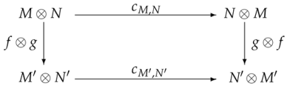
We will first show that the braiding c is natural. For all $(M^{\prime },{\alpha }_{M^{\prime }},{\beta }_{M^{\prime }},{\psi }_{M^{\prime }},{\omega }_{M^{\prime }}),$$(N^{\prime },{\alpha }_{N^{\prime }},$ ${\beta }_{N^{\prime }},{\psi }_{N^{\prime }},{\omega }_{N^{\prime }})\in {}_H^H\mathcal{BHYD}$, let $f:M\to M^{\prime },g:N\to N^{\prime }$ be morphisms in ${}_H^H\mathcal{BHYD}$ and consider the diagram

      

For all $m\in M,n\in N$, since the morphism g is left H-linear and f is left H-colinear, we obtain

$$\begin{array}{ccc}& & (g\otimes f)\circ c_{M,N}(m\otimes n)\hfill \\ & =& g({\alpha }_H^{-1}{\omega }_H^{-1}\left(m_{(-1)}\right)·{\beta }_N^{-1}\left(n\right))\otimes f\left({\psi }_M^{-1}\left(m_{\left(0\right)}\right)\right)\hfill \\ & =& {\alpha }_H^{-1}{\omega }_H^{-1}\left(m_{(-1)}\right)·g\left({\beta }_N^{-1}\left(n\right)\right)\otimes f\left({\psi }_M^{-1}\left(m_{\left(0\right)}\right)\right)\hfill \\ & =& {\alpha }_H^{-1}{\omega }_H^{-1}\left(m_{(-1)}\right)·{\beta }_{N^{\prime }}^{-1}\left(g\left(n\right)\right)\otimes {\psi }_{M^{\prime }}^{-1}\left(f\left(m_{\left(0\right)}\right)\right)\hfill \\ & =& {\alpha }_H^{-1}{\omega }_H^{-1}\left(f{\left(m\right)}_{(-1)}\right)·{\beta }_{N^{\prime }}^{-1}\left(g\left(n\right)\right)\otimes {\psi }_{M^{\prime }}^{-1}\left(f{\left(m\right)}_{\left(0\right)}\right)\hfill \\ & =& c_{M^{\prime },N^{\prime }}(f\left(m\right)\otimes g\left(n\right))\hfill \\ & =& c_{M^{\prime },N^{\prime }}\circ (f\otimes g)(m\otimes n).\hfill \end{array}$$

This follows $(g\otimes f)\circ c_{M,N}=c_{M^{\prime },N^{\prime }}\circ (f\otimes g)$, and the diagram commutes.

Next, we prove the H-linear of $c_{M,N}$:

$$\begin{array}{ccc}& & c_{M,N}(h·(m\otimes n))\hfill \\ & =& c_{M,N}({\omega }_H^{-1}\left(h_1\right)·m\otimes {\psi }_H^{-1}\left(h_2\right)·n)\hfill \\ & =& {\alpha }_H^{-1}{\omega }_H^{-1}\left({({\omega }_H^{-1}\left(h_1\right)·m)}_{(-1)}\right)·{\beta }_N^{-1}({\psi }_H^{-1}\left(h_2\right)·n)\otimes {\psi }_M^{-1}\left({({\omega }_H^{-1}\left(h_1\right)·m)}_{\left(0\right)}\right)\hfill \\ & \stackrel{\left(10\right)}{=}& {\alpha }_H^{-1}{\omega }_H^{-1}\left[\left({\alpha }_H^{-1}{\omega }_H^{-2}\left(h_{111}\right){\alpha }_H^{-1}\left(m_{(-1)}\right)\right){\alpha }_H{\beta }_H^{-1}{\psi }_H^{-1}{S}_H\left(h_{12}\right)\right]·({\beta }_H^{-1}{\psi }_H^{-1}\left(h_2\right)·{\beta }_N^{-1}\left(n\right))\hfill \\ & & \otimes {\psi }_H^{-1}{\omega }_H^{-2}\left(h_{112}\right)·{\psi }_M^{-1}\left(m_{\left(0\right)}\right)\hfill \\ & \stackrel{\left(2\right)}{=}& \left({\alpha }_H^{-1}{\omega }_H^{-3}\left(h_{111}\right){\alpha }_H^{-1}{\omega }_H^{-1}\left(m_{(-1)}\right)\right)·[{\beta }_H^{-1}{\psi }_H^{-1}{\omega }_H^{-1}{S}_H\left(h_{12}\right)·({\beta }_H^{-2}{\psi }_H^{-1}\left(h_2\right)·{\beta }_N^{-2}\left(n\right))]\hfill \\ & & \otimes {\psi }_H^{-1}{\omega }_H^{-2}\left(h_{112}\right)·{\psi }_M^{-1}\left(m_{\left(0\right)}\right)\hfill \\ & \stackrel{\left(2\right)}{=}& \left({\alpha }_H^{-1}{\omega }_H^{-3}\left(h_{111}\right){\alpha }_H^{-1}{\omega }_H^{-1}\left(m_{(-1)}\right)\right)·[\left({\alpha }_H^{-1}{\beta }_H^{-1}{\psi }_H^{-1}{\omega }_H^{-1}{S}_H\left(h_{12}\right){\beta }_H^{-2}{\psi }_H^{-1}\left(h_2\right)\right)·{\beta }_N^{-1}\left(n\right)]\hfill \\ & & \otimes {\psi }_H^{-1}{\omega }_H^{-2}\left(h_{112}\right)·{\psi }_M^{-1}\left(m_{\left(0\right)}\right)\hfill \\ & \stackrel{\left(4\right)}{=}& \left({\alpha }_H^{-1}{\omega }_H^{-2}\left(h_{11}\right){\alpha }_H^{-1}{\omega }_H^{-1}\left(m_{(-1)}\right)\right)·[\left({\alpha }_H^{-1}{\beta }_H^{-1}{\psi }_H^{-1}{\omega }_H^{-1}{S}_H\left(h_{21}\right){\beta }_H^{-2}{\psi }_H^{-2}\left(h_{22}\right)\right)·{\beta }_N^{-1}\left(n\right)]\hfill \\ & & \otimes {\psi }_H^{-1}{\omega }_H^{-1}\left(h_{12}\right)·{\psi }_M^{-1}\left(m_{\left(0\right)}\right)\hfill \\ & =& \left({\alpha }_H^{-1}{\omega }_H^{-2}\left(h_{11}\right){\alpha }_H^{-1}{\omega }_H^{-1}\left(m_{(-1)}\right)\right)·\left[\right({\beta }_H{\psi }_H{S}_H\left({\alpha }_H^{-1}{\beta }_H^{-2}{\psi }_H^{-2}{\omega }_H^{-1}\left(h_{21}\right)\right)\hfill \\ & & {\alpha }_H{\omega }_H\left({\alpha }_H^{-1}{\beta }_H^{-2}{\psi }_H^{-2}{\omega }_H^{-1}\left(h_{22}\right)\right))·{\beta }_N^{-1}\left(n\right)]\otimes {\psi }_H^{-1}{\omega }_H^{-1}\left(h_{12}\right)·{\psi }_M^{-1}\left(m_{\left(0\right)}\right)\hfill \\ & \stackrel{\left(6\right)}{=}& \left({\alpha }_H^{-1}{\omega }_H^{-2}\left(h_{11}\right){\alpha }_H^{-1}{\omega }_H^{-1}\left(m_{(-1)}\right)\right)·[{\epsilon }_H\left(h_2\right)1_H·{\beta }_N^{-1}\left(n\right)]\otimes {\psi }_H^{-1}{\omega }_H^{-1}\left(h_{12}\right)·{\psi }_M^{-1}\left(m_{\left(0\right)}\right)\hfill \\ & =& \left({\alpha }_H^{-1}{\omega }_H^{-1}\left(h_1\right){\alpha }_H^{-1}{\omega }_H^{-1}\left(m_{(-1)}\right)\right)·n\otimes {\psi }_H^{-1}\left(h_2\right)·{\psi }_M^{-1}\left(m_{\left(0\right)}\right)\hfill \\ & \stackrel{\left(2\right)}{=}& {\omega }_H^{-1}\left(h_1\right)·({\alpha }_H^{-1}{\omega }_H^{-1}\left(m_{(-1)}\right)·{\beta }_N^{-1}\left(n\right))\otimes {\psi }_H^{-1}\left(h_2\right)·{\psi }_M^{-1}\left(m_{\left(0\right)}\right)\hfill \\ & =& h·({\alpha }_H^{-1}{\omega }_H^{-1}\left(m_{(-1)}\right)·{\beta }_N^{-1}\left(n\right)\otimes {\psi }_M^{-1}\left(m_{\left(0\right)}\right))\hfill \\ & =& h·c_{M,N}(m\otimes n)\hfill \end{array}$$

and H-colinear of $c_{M,N}$:

$$\begin{array}{ccc}& & {\rho }_{N\otimes M}\circ c_{M,N}(m\otimes n)\hfill \\ & =& {\rho }_{N\otimes M}({\alpha }_H^{-1}{\omega }_H^{-1}\left(m_{(-1)}\right)·{\beta }_N^{-1}\left(n\right)\otimes {\psi }_M^{-1}\left(m_{\left(0\right)}\right))\hfill \\ & =& {\alpha }_H^{-1}\left({({\alpha }_H^{-1}{\omega }_H^{-1}\left(m_{(-1)}\right)·{\beta }_N^{-1}\left(n\right))}_{(-1)}\right){\beta }_H^{-1}\left({\psi }_M^{-1}{\left(m_{\left(0\right)}\right)}_{(-1)}\right)\otimes {({\alpha }_H^{-1}{\omega }_H^{-1}\left(m_{(-1)}\right)·{\beta }_N^{-1}\left(n\right))}_{\left(0\right)}\hfill \\ & & \otimes {\psi }_M^{-1}{\left(m_{\left(0\right)}\right)}_{\left(0\right)}\hfill \\ & \stackrel{\left(10\right)}{=}& {\alpha }_H^{-1}\left[\left({\alpha }_H^{-2}{\omega }_H^{-2}\left(m_{(-1)11}\right){\alpha }_H^{-1}{\beta }_H^{-1}\left(n_{(-1)}\right)\right){\beta }_H^{-1}{\psi }_H^{-1}{S}_H\left(m_{(-1)2}\right)\right]{\beta }_H^{-1}{\psi }_H^{-1}\left(m_{\left(0\right)(-1)}\right)\hfill \\ & & \otimes {\alpha }_H^{-1}{\omega }_H^{-2}\left(m_{(-1)12}\right)·{\beta }_N^{-1}\left(n_{\left(0\right)}\right)\otimes {\psi }_M^{-1}\left(m_{\left(0\right)\left(0\right)}\right)\hfill \\ & \stackrel{\left(1\right)}{=}& \left({\alpha }_H^{-2}{\omega }_H^{-2}\left(m_{(-1)11}\right){\alpha }_H^{-1}{\beta }_H^{-1}\left(n_{(-1)}\right)\right)\left[{\alpha }_H^{-1}{\beta }_H^{-1}{\psi }_H^{-1}{S}_H\left(m_{(-1)2}\right){\beta }_H^{-2}{\psi }_H^{-1}\left(m_{\left(0\right)(-1)}\right)\right]\hfill \\ & & \otimes {\alpha }_H^{-1}{\omega }_H^{-2}\left(m_{(-1)12}\right)·{\beta }_N^{-1}\left(n_{\left(0\right)}\right)\otimes {\psi }_M^{-1}\left(m_{\left(0\right)\left(0\right)}\right)\hfill \\ & \stackrel{\left(5\right)}{=}& \left({\alpha }_H^{-2}{\omega }_H^{-3}\left(m_{(-1)111}\right){\alpha }_H^{-1}{\beta }_H^{-1}\left(n_{(-1)}\right)\right)\left[{\alpha }_H^{-1}{\beta }_H^{-1}{\psi }_H^{-1}{\omega }_H^{-1}{S}_H\left(m_{(-1)12}\right){\beta }_H^{-2}{\psi }_H^{-1}\left(m_{(-1)2}\right)\right]\hfill \\ & & \otimes {\alpha }_H^{-1}{\omega }_H^{-3}\left(m_{(-1)112}\right)·{\beta }_N^{-1}\left(n_{\left(0\right)}\right)\otimes m_{\left(0\right)}\hfill \\ & \stackrel{(4)}{=}& \left({\alpha }_H^{-2}{\omega }_H^{-2}\left(m_{(-1)11}\right){\alpha }_H^{-1}{\beta }_H^{-1}\left(n_{(-1)}\right)\right)\left[{\alpha }_H^{-1}{\beta }_H^{-1}{\psi }_H^{-1}{\omega }_H^{-1}{S}_H\left(m_{(-1)21}\right){\beta }_H^{-2}{\psi }_H^{-2}\left(m_{(-1)22}\right)\right]\hfill \\ & & \otimes {\alpha }_H^{-1}{\omega }_H^{-2}\left(m_{(-1)12}\right)·{\beta }_N^{-1}\left(n_{\left(0\right)}\right)\otimes m_{\left(0\right)}\hfill \\ & =& \left({\alpha }_H^{-2}{\omega }_H^{-2}\left(m_{(-1)11}\right){\alpha }_H^{-1}{\beta }_H^{-1}\left(n_{(-1)}\right)\right)[{\beta }_H{\psi }_H{S}_H\left({\alpha }_H^{-1}{\beta }_H^{-2}{\psi }_H^{-2}{\omega }_H^{-1}\left(m_{(-1)21}\right)\right)\hfill \\ & & {\alpha }_H{\omega }_H\left({\alpha }_H^{-1}{\beta }_H^{-2}{\psi }_H^{-2}{\omega }_H^{-1}\left(m_{(-1)22}\right)\right)]\otimes {\alpha }_H^{-1}{\omega }_H^{-2}\left(m_{(-1)12}\right)·{\beta }_N^{-1}\left(n_{\left(0\right)}\right)\otimes m_{\left(0\right)}\hfill \\ & \stackrel{\left(6\right)}{=}& \left({\alpha }_H^{-2}{\omega }_H^{-2}\left(m_{(-1)11}\right){\alpha }_H^{-1}{\beta }_H^{-1}\left(n_{(-1)}\right)\right){\epsilon }_H\left(m_{(-1)2}\right)1_H\otimes {\alpha }_H^{-1}{\omega }_H^{-2}\left(m_{(-1)12}\right)·{\beta }_N^{-1}\left(n_{\left(0\right)}\right)\otimes m_{\left(0\right)}\hfill \\ & =& {\alpha }_H^{-1}{\omega }_H^{-1}\left(m_{(-1)1}\right){\beta }_H^{-1}\left(n_{(-1)}\right)\otimes {\alpha }_H^{-1}{\omega }_H^{-1}\left(m_{(-1)2}\right)·{\beta }_N^{-1}\left(n_{\left(0\right)}\right)\otimes m_{\left(0\right)}\hfill \\ & \stackrel{\left(5\right)}{=}& {\alpha }_H^{-1}\left(m_{(-1)}\right){\beta }_H^{-1}\left(n_{(-1)}\right)\otimes {\alpha }_H^{-1}{\omega }_H^{-1}\left(m_{\left(0\right)(-1)}\right)·{\beta }_N^{-1}\left(n_{\left(0\right)}\right)\otimes {\psi }_M^{-1}\left(m_{\left(0\right)\left(0\right)}\right)\hfill \\ & =& {\alpha }_H^{-1}\left(m_{(-1)}\right){\beta }_H^{-1}\left(n_{(-1)}\right)\otimes c_{M,N}(m_{\left(0\right)}\otimes n_{\left(0\right)})\hfill \\ & =& (i{d}_H\otimes c_{M,N})\circ {\rho }_{M\otimes N}(m\otimes n).\hfill \end{array}$$

Now, we prove $c_{M,N}$ is an isomorphism with an inverse map

$$\begin{array}{ccc}\hfill c_{M,N}^{-1}:& & N\otimes M\to M\otimes N,\hfill \\ & & n\otimes m\mapsto {\psi }_M^{-1}\left(m_{\left(0\right)}\right)\otimes S_H^{-1}\left({\alpha }_H^{-1}{\omega }_H^{-1}\left(m_{(-1)}\right)\right)·{\beta }_N^{-1}\left(n\right).\hfill \end{array}$$

For all $m\in M$ and $n\in N$, we compute

$$\begin{array}{ccc}& & c_{M,N}^{-1}\circ c_{M,N}(m\otimes n)\hfill \\ & =& c_{M,N}^{-1}({\alpha }_H^{-1}{\omega }_H^{-1}\left(m_{(-1)}\right)·{\beta }_N^{-1}\left(n\right)\otimes {\psi }_M^{-1}\left(m_{\left(0\right)}\right))\hfill \\ & =& {\psi }_M^{-2}\left(m_{\left(0\right)\left(0\right)}\right)\otimes S_H^{-1}\left({\alpha }_H^{-1}{\psi }_H^{-1}{\omega }_H^{-1}\left(m_{\left(0\right)(-1)}\right)\right)·({\alpha }_H^{-1}{\beta }_H^{-1}{\omega }_H^{-1}\left(m_{(-1)}\right)·{\beta }_N^{-2}\left(n\right))\hfill \\ & \stackrel{\left(2\right)}{=}& {\psi }_M^{-2}\left(m_{\left(0\right)\left(0\right)}\right)\otimes \left[S_H^{-1}{\alpha }_H^{-2}{\psi }_H^{-1}{\omega }_H^{-1}\left(m_{\left(0\right)(-1)}\right){\alpha }_H^{-1}{\beta }_H^{-1}{\omega }_H^{-1}\left(m_{(-1)}\right)\right]·{\beta }_N^{-1}\left(n\right)\hfill \\ & \stackrel{\left(5\right)}{=}& {\psi }_M^{-1}\left(m_{\left(0\right)}\right)\otimes \left[S_H^{-1}{\alpha }_H^{-2}{\psi }_H^{-1}{\omega }_H^{-1}\left(m_{(-1)2}\right){\alpha }_H^{-1}{\beta }_H^{-1}{\omega }_H^{-2}\left(m_{(-1)1}\right)\right]·{\beta }_N^{-1}\left(n\right)\hfill \\ & =& {\psi }_M^{-1}\left(m_{\left(0\right)}\right)\otimes \left[{\beta }_H{\omega }_H\left({\alpha }_H^{-2}{\beta }_H^{-1}{\psi }_H^{-1}{\omega }_H^{-2}{S}_H^{-1}\left(m_{(-1)2}\right)\right){\alpha }_H{\psi }_H\left({\alpha }_H^{-2}{\beta }_H^{-1}{\psi }_H^{-1}{\omega }_H^{-2}\left(m_{(-1)1}\right)\right)\right]\hfill \\ & & ·{\beta }_N^{-1}\left(n\right)\hfill \\ & \stackrel{\left(6\right)}{=}& {\psi }_M^{-1}\left(m_{\left(0\right)}\right)\otimes {\epsilon }_H\left(m_{(-1)}\right)1_H·{\beta }_N^{-1}\left(n\right)\hfill \\ & =& m\otimes n.\hfill \end{array}$$

Similarly, we can prove $c_{M,N}\circ c_{M,N}^{-1}=i{d}_{N\otimes M}$.

Finally, let us verify the hexagon axioms from [9], XIII.1.1. For any $(U,{\alpha }_U,{\beta }_U,{\psi }_U,{\omega }_U),$$(V,{\alpha }_V,{\beta }_V,{\psi }_V,{\omega }_V),(W,{\alpha }_W,{\beta }_W,{\psi }_W,{\omega }_W)\in {}_H^H\mathcal{BHYD}$, we compute

$$\begin{array}{ccc}& & (i{d}_V\otimes c_{U,W})(c_{U,V}\otimes i{d}_W)(u\otimes v\otimes w)\hfill \\ & =& (i{d}_V\otimes c_{U,W})({\alpha }_H^{-1}{\omega }_H^{-1}\left(u_{(-1)}\right)·{\beta }_V^{-1}\left(v\right)\otimes {\psi }_U^{-1}\left(u_{\left(0\right)}\right)\otimes w)\hfill \\ & =& {\alpha }_H^{-1}{\omega }_H^{-1}\left(u_{(-1)}\right)·{\beta }_V^{-1}\left(v\right)\otimes {\alpha }_H^{-1}{\psi }_H^{-1}{\omega }_H^{-1}\left(u_{\left(0\right)(-1)}\right)·{\beta }_W^{-1}\left(w\right)\otimes {\psi }_U^{-2}\left(u_{\left(0\right)\left(0\right)}\right)\hfill \\ & \stackrel{\left(5\right)}{=}& {\alpha }_H^{-1}{\omega }_H^{-2}\left(u_{(-1)1}\right)·{\beta }_V^{-1}\left(v\right)\otimes {\alpha }_H^{-1}{\psi }_H^{-1}{\omega }_H^{-1}\left(u_{(-1)2}\right)·{\beta }_W^{-1}\left(w\right)\otimes {\psi }_U^{-1}\left(u_{\left(0\right)}\right)\hfill \\ & =& {\omega }_H^{-1}\left({\alpha }_H^{-1}{\omega }_H^{-1}\left(u_{(-1)1}\right)\right)·{\beta }_V^{-1}\left(v\right)\otimes {\psi }_H^{-1}\left({\alpha }_H^{-1}{\omega }_H^{-1}\left(u_{(-1)2}\right)\right)·{\beta }_W^{-1}\left(w\right)\otimes {\psi }_U^{-1}\left(u_{\left(0\right)}\right)\hfill \\ & =& {\alpha }_H^{-1}{\omega }_H^{-1}\left(u_{(-1)}\right)·({\beta }_V^{-1}\left(v\right)\otimes {\beta }_W^{-1}\left(w\right))\otimes {\psi }_U^{-1}\left(u_{\left(0\right)}\right)\hfill \\ & =& {\alpha }_H^{-1}{\omega }_H^{-1}\left(u_{(-1)}\right)·{\beta }_{V\otimes W}^{-1}(v\otimes w)\otimes {\psi }_U^{-1}\left(u_{\left(0\right)}\right)\hfill \\ & =& c_{U,V\otimes W}(u\otimes (v\otimes w))\hfill \end{array}$$

and

$$\begin{array}{ccc}& & (c_{U,W}\otimes i{d}_V)(i{d}_U\otimes c_{V,W})(u\otimes v\otimes w)\hfill \\ & =& (c_{U,W}\otimes i{d}_V)(u\otimes {\alpha }_H^{-1}{\omega }_H^{-1}\left(v_{(-1)}\right)·{\beta }_W^{-1}\left(w\right)\otimes {\psi }_V^{-1}\left(v_{\left(0\right)}\right))\hfill \\ & =& {\alpha }_H^{-1}{\omega }_H^{-1}\left(u_{(-1)}\right)·({\alpha }_H^{-1}{\beta }_H^{-1}{\omega }_H^{-1}\left(v_{(-1)}\right)·{\beta }_W^{-2}\left(w\right))\otimes {\psi }_U^{-1}\left(u_{\left(0\right)}\right)\otimes {\psi }_V^{-1}\left(v_{\left(0\right)}\right)\hfill \\ & \stackrel{\left(2\right)}{=}& \left({\alpha }_H^{-2}{\omega }_H^{-1}\left(u_{(-1)}\right){\alpha }_H^{-1}{\beta }_H^{-1}{\omega }_H^{-1}\left(v_{(-1)}\right)\right)·{\beta }_W^{-1}\left(w\right)\otimes {\psi }_{U\otimes V}^{-1}(u_{\left(0\right)}\otimes v_{\left(0\right)})\hfill \\ & =& {\alpha }_H^{-1}{\omega }_H^{-1}\left({\alpha }_H^{-1}\left(u_{(-1)}\right){\beta }_H^{-1}\left(v_{(-1)}\right)\right)·{\beta }_W^{-1}\left(w\right)\otimes {\psi }_{U\otimes V}^{-1}\left({(u\otimes v)}_{\left(0\right)}\right)\hfill \\ & =& {\alpha }_H^{-1}{\omega }_H^{-1}\left({(u\otimes v)}_{(-1)}\right)·{\beta }_W^{-1}\left(w\right)\otimes {\psi }_{U\otimes V}^{-1}\left({(u\otimes v)}_{\left(0\right)}\right)\hfill \\ & =& c_{U\otimes V,W}((u\otimes v)\otimes w).\hfill \end{array}$$

The proof is finished. □

We discuss the connection between left–left BiHom–Yetter–Drinfeld modules and co-modules over coquasitriangular BiHom-bialgebras in the following proposition. According to the definition of coquasitriangular bialgebra in [12], we can generate the BiHom-case:

Definition 8.

Let $(H,{\mu }_H,{\Delta }_H,{\alpha }_H,{\beta }_H,{\psi }_H,{\omega }_H)$ be a BiHom-bialgebra and $\sigma :H\otimes H\to k$ a linear map. We call $(H,\sigma )$ a coquasitriangular BiHom-bialgebra if, for all $x,y,z\in H$, we have

$$\begin{array}{ccc}& & \sigma (xy\otimes {\psi }_H{\omega }_H\left(z\right))=\sigma ({\alpha }_H\left(x\right)\otimes {\psi }_H\left(z_1\right))\sigma ({\beta }_H\left(y\right)\otimes {\omega }_H\left(z_2\right)),\hfill \end{array}$$

(11)

$$\sigma ({\psi }_H{\omega }_H\left(x\right)\otimes yz)=\sigma ({\psi }_H\left(x_1\right)\otimes {\beta }_H\left(z\right))\sigma ({\omega }_H\left(x_2\right)\otimes {\alpha }_H\left(y\right)),$$

(12)

$$\begin{array}{cc}& {\beta }_H{\psi }_H\left(y_1\right){\alpha }_H{\psi }_H\left(x_1\right)\sigma ({\alpha }_H{\beta }_H{\omega }_H\left(x_2\right)\otimes {\alpha }_H{\beta }_H{\omega }_H\left(y_2\right))\hfill \\ \hfill =& \sigma ({\alpha }_H{\beta }_H{\psi }_H\left(x_1\right)\otimes {\alpha }_H{\beta }_H{\psi }_H\left(y_1\right)){\beta }_H{\omega }_H\left(x_2\right){\alpha }_H{\omega }_H\left(y_2\right).\hfill \end{array}$$

(13)

Proposition 3.

Let $(H,{\mu }_H,{\Delta }_H,{\alpha }_H,{\beta }_H,{\psi }_H,{\omega }_H,\sigma )$ be a coquasitriangular BiHom-bialgebra with the ${\alpha }_H,{\beta }_H,{\psi }_H,{\omega }_H$ bijective, which satisfies the following condition

$$\begin{array}{c}\hfill \sigma ({\omega }_H\left(x\right)\otimes {\alpha }_H\left(y\right))=\sigma ({\psi }_H\left(x\right)\otimes {\beta }_H\left(y\right))=\sigma (x\otimes y),\end{array}$$

(14)

for all $x,y,z\in H$.

$\left(i\right)$ If $(M,{\psi }_M,{\omega }_M)$ is a left H-co-module with coaction $M\to H\otimes M,m\mapsto m_{(-1)}\otimes m_{\left(0\right)}$, define a new linear map $·:H\otimes M\to M$ as $h·m=\sigma ({\alpha }_H{\beta }_H{\psi }_H\left(m_{(-1)}\right)\otimes {\alpha }_H^2{\psi }_H{\omega }_H\left(h\right))m_{\left(0\right)}$, then $(M,{\omega }_M,{\psi }_M,{\psi }_M,{\omega }_M)$, along with these structures, forms a left–left BiHom–Yetter–Drinfeld module over H.

$\left(ii\right)$ If $(N,{\psi }_N,{\omega }_N)$ is another left H-co-module with coaction $\rho :N\to H\otimes N$ defined by $\rho \left(n\right)=n_{(-1)}\otimes n_{\left(0\right)}$, followed by a left–left BiHom–Yetter–Drinfeld module as in (i), via the module action $H\otimes N\to N,h·n=\sigma ({\alpha }_H{\beta }_H{\psi }_H\left(n_{(-1)}\right)\otimes {\alpha }_H^2{\psi }_H{\omega }_H\left(h\right))n_{\left(0\right)}$, then we regard $(M\otimes N,{\psi }_M\otimes {\psi }_N,{\omega }_M\otimes {\omega }_N)$ as a left H-co-module via the action $\rho (m\otimes n)={\alpha }_H^{-1}\left(m_{(-1)}\right){\beta }_H^{-1}\left(n_{(-1)}\right)\otimes m_{\left(0\right)}\otimes n_{\left(0\right)}$ and $(M\otimes N,{\psi }_M\otimes {\psi }_N,{\omega }_M\otimes {\omega }_N)$ as a left–left BiHom–Yetter–Drinfeld module as in (i). This BiHom–Yetter–Drinfeld module $(M\otimes N,{\psi }_M\otimes {\psi }_N,{\omega }_M\otimes {\omega }_N)$ coincides with the BiHom–Yetter–Drinfeld modules $M\widehat{\otimes }N$ defined above in Theorem 1.

Proof. 

(i) First, we must prove that $(M,{\omega }_M,{\psi }_M)$ is a left H-module. For all $h,h^{\prime }\in H,m\in M$, we check Equation (2) as follows:

$$\begin{array}{ccc}& & {\alpha }_H\left(h\right)·(h^{\prime }·m)\hfill \\ & =& {\alpha }_H\left(h\right)·m_{\left(0\right)}\sigma ({\alpha }_H{\beta }_H{\psi }_H\left(m_{(-1)}\right)\otimes {\alpha }_H^2{\psi }_H{\omega }_H\left(h^{\prime }\right))\hfill \\ & =& \sigma ({\alpha }_H{\beta }_H{\psi }_H\left(m_{(-1)}\right)\otimes {\alpha }_H^2{\psi }_H{\omega }_H\left(h^{\prime }\right))\sigma ({\alpha }_H{\beta }_H{\psi }_H\left(m_{\left(0\right)(-1)}\right)\otimes {\alpha }_H^2{\psi }_H{\omega }_H\left({\alpha }_H\left(h\right)\right))m_{\left(0\right)\left(0\right)}\hfill \\ & \stackrel{\left(5\right)}{=}& \sigma ({\alpha }_H{\beta }_H{\psi }_H{\omega }_H^{-1}\left(m_{(-1)1}\right)\otimes {\alpha }_H^2{\psi }_H{\omega }_H\left(h^{\prime }\right))\hfill \\ & & \sigma ({\alpha }_H{\beta }_H{\psi }_H\left(m_{(-1)2}\right)\otimes {\alpha }_H^2{\psi }_H{\omega }_H\left({\alpha }_H\left(h\right)\right)){\psi }_M\left(m_{\left(0\right)}\right)\hfill \\ & \stackrel{\left(14\right)}{=}& \sigma ({\psi }_H\left({\alpha }_H{\beta }_H{\psi }_H{\omega }_H^{-1}\left(m_{(-1)1}\right)\right)\otimes {\beta }_H\left({\alpha }_H^2{\psi }_H{\omega }_H\left(h^{\prime }\right)\right))\sigma ({\omega }_H\left({\alpha }_H{\beta }_H{\psi }_H{\omega }_H^{-1}\left(m_{(-1)2}\right)\right)\hfill \\ & & \otimes {\alpha }_H\left({\alpha }_H^2{\psi }_H{\omega }_H\left(h\right)\right)){\psi }_M\left(m_{\left(0\right)}\right)\hfill \\ & \stackrel{\left(12\right)}{=}& \sigma ({\psi }_H{\omega }_H\left({\alpha }_H{\beta }_H{\psi }_H{\omega }_H^{-1}\left(m_{(-1)}\right)\right)\otimes {\alpha }_H^2{\psi }_H{\omega }_H\left(h{h}^{\prime }\right)){\psi }_M\left(m_{\left(0\right)}\right)\hfill \\ & =& \sigma ({\alpha }_H{\beta }_H{\psi }_H\left({\psi }_H\left(m_{(-1)}\right)\right)\otimes {\alpha }_H^2{\psi }_H{\omega }_H\left(h{h}^{\prime }\right)){\psi }_M\left(m_{\left(0\right)}\right)\hfill \\ & =& \left(h{h}^{\prime }\right)·{\psi }_M\left(m\right).\hfill \end{array}$$

Now, we check if $(M,{\omega }_M,{\psi }_M,{\psi }_M,{\omega }_M)$ is a left–left BiHom–Yetter–Drinfeld module. In this case, the compatibility condition Equation (9) changes to

$$\begin{array}{ccc}& & {\beta }_H{\psi }_H\left({({\psi }_H\left(h_1\right)·m)}_{(-1)}\right){\alpha }_H^2{\psi }_H{\omega }_H^2\left(h_2\right)\otimes {({\psi }_H\left(h_1\right)·m)}_{\left(0\right)}\hfill \\ & =& {\alpha }_H{\beta }_H{\psi }_H^2{\omega }_H\left(h_1\right){\alpha }_H{\psi }_H^2\left(m_{(-1)}\right)\otimes {\beta }_H{\omega }_H\left(h_2\right)·m_{\left(0\right)},\hfill \end{array}$$

for all $h\in H$ and $m\in M$. We compute:

$$\begin{array}{ccc}& & {\alpha }_H{\beta }_H{\psi }_H^2{\omega }_H\left(h_1\right){\alpha }_H{\psi }_H^2\left(m_{(-1)}\right)\otimes {\beta }_H{\omega }_H\left(h_2\right)·m_{\left(0\right)}\hfill \\ & =& {\alpha }_H{\beta }_H{\psi }_H^2{\omega }_H\left(h_1\right){\alpha }_H{\psi }_H^2\left(m_{(-1)}\right)\otimes \sigma ({\alpha }_H{\beta }_H{\psi }_H\left(m_{\left(0\right)(-1)}\right)\otimes {\alpha }_H^2{\psi }_H{\omega }_H\left({\beta }_H{\omega }_H\left(h_2\right)\right))m_{\left(0\right)\left(0\right)}\hfill \\ & \stackrel{\left(5\right)}{=}& {\alpha }_H{\beta }_H{\psi }_H^2{\omega }_H\left(h_1\right){\alpha }_H{\psi }_H^2{\omega }_H^{-1}\left(m_{(-1)1}\right)\sigma ({\alpha }_H{\beta }_H{\psi }_H\left(m_{(-1)2}\right)\otimes {\alpha }_H^2{\beta }_H{\psi }_H{\omega }_H^2\left(h_2\right))\otimes {\psi }_M\left(m_{\left(0\right)}\right)\hfill \\ & =& {\beta }_H{\psi }_H\left({\alpha }_H{\psi }_H{\omega }_H\left(h_1\right)\right){\alpha }_H{\psi }_H\left({\psi }_H{\omega }_H^{-1}\left(m_{(-1)1}\right)\right)\sigma ({\alpha }_H{\beta }_H{\omega }_H\left({\psi }_H{\omega }_H^{-1}\left(m_{(-1)2}\right)\right)\hfill \\ & & \otimes {\alpha }_H{\beta }_H{\omega }_H\left({\alpha }_H{\psi }_H{\omega }_H\left(h_2\right)\right))\otimes {\psi }_M\left(m_{\left(0\right)}\right)\hfill \\ & \stackrel{\left(13\right)}{=}& \sigma ({\alpha }_H{\beta }_H{\psi }_H\left({\psi }_H{\omega }_H^{-1}\left(m_{(-1)1}\right)\right)\otimes {\alpha }_H{\beta }_H{\psi }_H\left({\alpha }_H{\psi }_H{\omega }_H\left(h_1\right)\right))\hfill \\ & & {\beta }_H{\omega }_H\left({\psi }_H{\omega }_H^{-1}\left(m_{(-1)2}\right)\right){\alpha }_H{\omega }_H\left({\alpha }_H{\psi }_H{\omega }_H\left(h_2\right)\right)\otimes {\psi }_M\left(m_{\left(0\right)}\right)\hfill \\ & =& \sigma ({\alpha }_H{\beta }_H{\psi }_H^2{\omega }_H^{-1}\left(m_{(-1)1}\right)\otimes {\alpha }_H^2{\beta }_H{\psi }_H^2{\omega }_H\left(h_1\right)){\beta }_H{\psi }_H\left(m_{(-1)2}\right){\alpha }_H^2{\psi }_H{\omega }_H^2\left(h_2\right)\otimes {\psi }_M\left(m_{\left(0\right)}\right)\hfill \\ & \stackrel{\left(5\right)}{=}& \sigma ({\alpha }_H{\beta }_H{\psi }_H^2\left(m_{(-1)}\right)\otimes {\alpha }_H^2{\beta }_H{\psi }_H^2{\omega }_H\left(h_1\right)){\beta }_H{\psi }_H\left(m_{\left(0\right)(-1)}\right){\alpha }_H^2{\psi }_H{\omega }_H^2\left(h_2\right)\otimes m_{\left(0\right)\left(0\right)}\hfill \\ & \stackrel{\left(14\right)}{=}& {\beta }_H{\psi }_H\left(m_{\left(0\right)(-1)}\right){\alpha }_H^2{\psi }_H{\omega }_H^2\left(h_2\right)\otimes \sigma ({\alpha }_H{\beta }_H{\psi }_H\left(m_{(-1)}\right)\otimes {\alpha }_H^2{\psi }_H^2{\omega }_H\left(h_1\right))m_{\left(0\right)\left(0\right)}\hfill \\ & =& {\beta }_H{\psi }_H\left(m_{\left(0\right)(-1)}\right){\alpha }_H^2{\psi }_H{\omega }_H^2\left(h_2\right)\otimes \sigma ({\alpha }_H{\beta }_H{\psi }_H\left(m_{(-1)}\right)\otimes {\alpha }_H^2{\psi }_H{\omega }_H\left({\psi }_H\left(h_1\right)\right))m_{\left(0\right)\left(0\right)}\hfill \\ & =& {\beta }_H{\psi }_H\left({({\psi }_H\left(h_1\right)·m)}_{(-1)}\right){\alpha }_H^2{\psi }_H{\omega }_H^2\left(h_2\right)\otimes {({\psi }_H\left(h_1\right)·m)}_{\left(0\right)}.\hfill \end{array}$$

(ii) From this, it is obvious that we have proven that the two module structures of $M\otimes N$ coincide, that is, for all $m\in M,n\in N$,

$$\begin{array}{c}\hfill {\omega }_H^{-1}\left(h_1\right)·m\otimes {\psi }_H^{-1}\left(h_2\right)·n=\sigma ({\alpha }_H{\beta }_H{\psi }_H\left({\alpha }_H^{-1}\left(m_{(-1)}\right){\beta }_H^{-1}\left(n_{(-1)}\right)\right)\otimes {\alpha }_H^2{\psi }_H{\omega }_H\left(h\right))m_{\left(0\right)}\otimes n_{\left(0\right)}.\end{array}$$

We compute

$$\begin{array}{ccc}& & {\omega }_H^{-1}\left(h_1\right)·m\otimes {\psi }_H^{-1}\left(h_2\right)·n\hfill \\ & =& \sigma ({\alpha }_H{\beta }_H{\psi }_H\left(m_{(-1)}\right)\otimes {\alpha }_H^2{\psi }_H\left(h_1\right))m_{\left(0\right)}\otimes \sigma ({\alpha }_H{\beta }_H{\psi }_H\left(n_{(-1)}\right)\otimes {\alpha }_H^2{\omega }_H\left(h_2\right))n_{\left(0\right)}\hfill \\ & =& \sigma ({\alpha }_H\left({\beta }_H{\psi }_H\left(m_{(-1)}\right)\right)\otimes {\psi }_H\left({\alpha }_H^2\left(h_1\right)\right))\sigma ({\beta }_H\left({\alpha }_H{\psi }_H\left(n_{(-1)}\right)\right)\otimes {\omega }_H\left({\alpha }_H^2\left(h_2\right)\right))m_{\left(0\right)}\otimes n_{\left(0\right)}\hfill \\ & \stackrel{\left(11\right)}{=}& \sigma ({\beta }_H{\psi }_H\left(m_{(-1)}\right){\alpha }_H{\psi }_H\left(n_{(-1)}\right)\otimes {\psi }_H{\omega }_H{\alpha }_H^2\left(h\right))m_{\left(0\right)}\otimes n_{\left(0\right)}\hfill \\ & =& \sigma ({\alpha }_H{\beta }_H{\psi }_H\left({\alpha }_H^{-1}\left(m_{(-1)}\right){\beta }_H^{-1}\left(n_{(-1)}\right)\right)\otimes {\alpha }_H^2{\psi }_H{\omega }_H\left(h\right))m_{\left(0\right)}\otimes n_{\left(0\right)},\hfill \end{array}$$

finishing the proof. □

As a consequence of the above results, we also obtain the following:

Theorem 2.

Let $(H,{\mu }_H,{\Delta }_H,{\alpha }_H,{\beta }_H,{\psi }_H,{\omega }_H,\sigma )$ be a coquasitriangular BiHom-bialgebra, where ${\alpha }_H,{\beta }_H,{\psi }_H,{\omega }_H$ are bijective and $\sigma =\sigma \circ ({\omega }_H\otimes {\alpha }_H)=\sigma \circ ({\psi }_H\otimes {\beta }_H)$ is true, as in Proposition 3. Denoted by ${}^H\mathcal{M}$, the category whose objects are left H-co-modules $(M,{\psi }_M,{\omega }_M)$ with ${\psi }_M,{\omega }_M$ bijective and morphisms are morphisms of left H-co-modules. Then, ${}^H\mathcal{M}$ is a braided monoidal subcategory of ${}_H^H\mathcal{BHYD}$ with a tensor product defined as $\rho :M\otimes N\to H\otimes M\otimes N,\rho (m\otimes n)={\alpha }_H^{-1}\left(m_{(-1)}\right){\beta }_H^{-1}\left(n_{(-1)}\right)\otimes m_{\left(0\right)}\otimes n_{\left(0\right)}$ and the braiding structure $c_{M,N}:M\otimes N\to N\otimes M,c_{M,N}(m\otimes n)=\sigma ({\alpha }_H{\beta }_H\left(n_{(-1)}\right)\otimes {\alpha }_H{\psi }_H\left(m_{(-1)}\right)){\psi }_N^{-1}\left(n_{\left(0\right)}\right)\otimes {\psi }_M^{-1}\left(m_{\left(0\right)}\right)$, for all $(M,{\psi }_M,{\omega }_M),(N,{\psi }_N,{\omega }_N)\in {}^H\mathcal{M}$.

4. The Duality of the Category of Finitely Generated Projective BiHom–Yetter–Drinfeld  Modules

In this section we will examine the idea that the category of finitely generated projective left–left BiHom–Yetter–Drinfeld modules has left and right duality. The definition of duality in a monoidal category can be found in [9,16].

Proposition 4.

Let $(H,{\mu }_H,{\Delta }_H,{\alpha }_H,{\beta }_H,{\psi }_H,{\omega }_H,S_H)$ be a BiHom–Hopf algebra with the maps ${\alpha }_H,{\beta }_H,{\psi }_H,{\omega }_H,S_H$ bijective and $(M,{\alpha }_M,{\beta }_M,{\psi }_M,{\omega }_M)$ be an object in the category ${}_H^H\mathcal{BHYD}$ and assume M is a finite dimensional. Then, $(M^{*}=Hom(M,\mathbb{k}),{\left({\alpha }_M^{*}\right)}^{-1},{\left({\beta }_M^{*}\right)}^{-1},{\left({\psi }_M^{*}\right)}^{-1},{\left({\omega }_M^{*}\right)}^{-1})$ is also a left–left BiHom–Yetter–Drinfeld module with the action

$$\begin{array}{c}\hfill (h\rightharpoonup f)\left(m\right)=f(S_H{\beta }_H^{-1}\left(h\right)·{\beta }_M^{-2}\left(m\right))\end{array}$$

and coaction

$$\begin{array}{c}\hfill \rho :M^{*}\to H\otimes M^{*},\rho \left(f\right)\triangleq f_{(-1)}\otimes f_{\left(0\right)},\end{array}$$

here $f_{(-1)}\otimes f_{\left(0\right)}\left(m\right)=S_H^{-1}{\psi }_H^{-1}\left(m_{(-1)}\right)\otimes f\left({\psi }_M^{-2}\left(m_{\left(0\right)}\right)\right)$, for all $h\in H,f\in M^{*}$ and $m\in M$.

Proof. 

We first check if $(M^{*},{\left({\alpha }_M^{*}\right)}^{-1},{\left({\beta }_M^{*}\right)}^{-1})$ is a left $(H,{\alpha }_H,{\beta }_H)$-module. We compute:

$$\begin{array}{ccc}\hfill ({\alpha }_H\left(h\right)\rightharpoonup {\left({\alpha }_M^{*}\right)}^{-1}\left(f\right))\left(m\right)& =& {\left({\alpha }_M^{*}\right)}^{-1}\left(f\right)(S_H{\alpha }_H{\beta }_H^{-1}\left(h\right)·{\beta }_M^{-2}\left(m\right))\hfill \\ & =& f(S_H{\beta }_H^{-1}\left(h\right)·{\alpha }_M^{-1}{\beta }_M^{-2}\left(m\right)),\hfill \\ \hfill {\left({\alpha }_M^{*}\right)}^{-1}(h\rightharpoonup f)\left(m\right)& =& (h\rightharpoonup f)\left({\alpha }_M^{-1}\left(m\right)\right)\hfill \\ & =& f(S_H{\beta }_H^{-1}\left(h\right)·{\beta }_M^{-2}{\alpha }_M^{-1}\left(m\right))\hfill \\ & =& f(S_H{\beta }_H^{-1}\left(h\right)·{\alpha }_M^{-1}{\beta }_M^{-2}\left(m\right)).\hfill \end{array}$$

It follows that ${\alpha }_H\left(h\right)\rightharpoonup {\left({\alpha }_M^{*}\right)}^{-1}\left(f\right)={\left({\alpha }_M^{*}\right)}^{-1}(h\rightharpoonup f)$. Similarly, we find ${\beta }_H\left(h\right)\rightharpoonup {\left({\beta }_M^{*}\right)}^{-1}\left(f\right)={\left({\beta }_M^{*}\right)}^{-1}(h\rightharpoonup f)$. For all $a,b\in H,f\in M^{*}$ and $m\in M$, we have

$$\begin{array}{ccc}& & (\left(ab\right)\rightharpoonup {\left({\beta }_M^{*}\right)}^{-1}\left(f\right))\left(m\right)\hfill \\ & =& {\left({\beta }_M^{*}\right)}^{-1}\left(f\right)(S_H{\beta }_H^{-1}\left(ab\right)·{\beta }_M^{-2}\left(m\right))\hfill \\ & =& f(S_H{\beta }_H^{-2}\left(ab\right)·{\beta }_M^{-3}\left(m\right))\hfill \\ & =& f[S_H\left({\beta }_H\left({\beta }_H^{-3}\left(a\right)\right){\alpha }_H\left({\alpha }_H^{-1}{\beta }_H^{-2}\left(b\right)\right)\right)·{\beta }_M^{-3}\left(m\right)]\hfill \\ & \stackrel{\left(7\right)}{=}& f[\left(S_H{\alpha }_H^{-1}{\beta }_H^{-1}\left(b\right)S_H{\alpha }_H{\beta }_H^{-3}\left(a\right)\right)·{\beta }_M^{-3}\left(m\right)]\hfill \\ & \stackrel{\left(2\right)}{=}& f[S_H\left({\beta }_H^{-1}\left(b\right)\right)·(S_H{\alpha }_H{\beta }_H^{-3}\left(a\right)·{\beta }_M^{-4}\left(m\right))]\hfill \\ & =& f[S_H\left({\beta }_H^{-1}\left(b\right)\right)·{\beta }_M^{-2}(S_H{\alpha }_H{\beta }_H^{-1}\left(a\right)·{\beta }_M^{-2}\left(m\right))]\hfill \\ & =& (b\rightharpoonup f)(S_H{\alpha }_H{\beta }_H^{-1}\left(a\right)·{\beta }_M^{-2}\left(m\right))\hfill \\ & =& (b\rightharpoonup f)(S_H{\beta }_H^{-1}\left({\alpha }_H\left(a\right)\right)·{\beta }_M^{-2}\left(m\right))\hfill \\ & =& ({\alpha }_H\left(a\right)\rightharpoonup (b\rightharpoonup f))\left(m\right).\hfill \end{array}$$

Next, we prove $((M,{\left({\psi }_M^{*}\right)}^{-1},{\left({\omega }_M^{*}\right)}^{-1})$ is a left $(H,{\psi }_H,{\omega }_H)$-co-module. For all $f\in M^{*}$ and $m\in M$, we obtain

$$\begin{array}{ccc}& & ({\psi }_H\otimes {\left({\psi }_M^{*}\right)}^{-1})\circ \rho \left(f\right)\hfill \\ & =& ({\psi }_H\otimes {\left({\psi }_M^{*}\right)}^{-1})(f_{(-1)}\otimes f_{\left(0\right)})\hfill \\ & =& {\psi }_H\left(f_{(-1)}\right)\otimes {\left({\psi }_M^{*}\right)}^{-1}\left(f_{\left(0\right)}\right)\left(m\right)\hfill \\ & =& S_H^{-1}{\psi }_H^{-1}\left(m_{(-1)}\right)\otimes f\left({\psi }_M^{-3}\left(m_{\left(0\right)}\right)\right)\hfill \\ & =& S_H^{-1}{\psi }_H^{-1}\left(m_{(-1)}\right)\otimes {\left({\psi }_M^{*}\right)}^{-1}\left(f\right)\left({\psi }_M^{-2}\left(m_{\left(0\right)}\right)\right)\hfill \\ & =& {\left({\left({\psi }_M^{*}\right)}^{-1}\left(f\right)\right)}_{(-1)}\otimes {\left({\left({\psi }_M^{*}\right)}^{-1}\left(f\right)\right)}_{\left(0\right)}\left(m\right)\hfill \\ & =& (\rho \circ {\left({\psi }_M^{*}\right)}^{-1})\left(f\right).\hfill \end{array}$$

Similarly, we have $({\omega }_H\otimes {\left({\omega }_M^{*}\right)}^{-1})\circ \rho =\rho \circ {\left({\omega }_M^{*}\right)}^{-1}$.

For all $f\in M^{*}$ and $m\in M$, we compute Equation (5):

$$\begin{array}{ccc}& & ({\Delta }_H\otimes {\left({\psi }_M^{*}\right)}^{-1})\circ \rho \left(f\right)\hfill \\ & =& f_{(-1)1}\otimes f_{(-1)2}\otimes {\left({\psi }_M^{*}\right)}^{-1}\left(f_{\left(0\right)}\right)\left(m\right)\hfill \\ & =& f_{(-1)1}\otimes f_{(-1)2}\otimes f_{\left(0\right)}\left({\psi }_M^{-1}\left(m\right)\right)\hfill \\ & =& {\left(S_H^{-1}{\psi }_H^{-2}\left(m_{(-1)}\right)\right)}_1\otimes {\left(S_H^{-1}{\psi }_H^{-2}\left(m_{(-1)}\right)\right)}_2\otimes f\left({\psi }_M^{-3}\left(m_{\left(0\right)}\right)\right)\hfill \\ & =& {\psi }_H^{-1}{\psi }_H{\left(S_H^{-1}{\psi }_H^{-2}\left(m_{(-1)}\right)\right)}_1\otimes {\omega }_H^{-1}{\omega }_H{\left(S_H^{-1}{\psi }_H^{-2}\left(m_{(-1)}\right)\right)}_2\otimes f\left({\psi }_M^{-3}\left(m_{\left(0\right)}\right)\right)\hfill \\ & \stackrel{\left(8\right)}{=}& {\psi }_H^{-1}{\omega }_H\left(S_H^{-1}{\psi }_H^{-2}\left(m_{(-1)2}\right)\right)\otimes {\psi }_H{\omega }_H^{-1}\left(S_H^{-1}{\psi }_H^{-2}\left(m_{(-1)1}\right)\right)\otimes f\left({\psi }_M^{-3}\left(m_{\left(0\right)}\right)\right)\hfill \\ & =& {\omega }_H{S}_H^{-1}{\psi }_H^{-3}\left(m_{(-1)2}\right)\otimes {\omega }_H^{-1}{S}_H^{-1}{\psi }_H^{-1}\left(m_{(-1)1}\right)\otimes f\left({\psi }_M^{-3}\left(m_{\left(0\right)}\right)\right)\hfill \\ & \stackrel{\left(5\right)}{=}& {\omega }_H{S}_H^{-1}{\psi }_H^{-3}\left(m_{\left(0\right)(-1)}\right)\otimes S_H^{-1}{\psi }_H^{-1}\left(m_{(-1)}\right)\otimes f\left({\psi }_M^{-4}\left(m_{\left(0\right)\left(0\right)}\right)\right)\hfill \\ & =& {\omega }_H\left(f_{(-1)}\right)\otimes S_H^{-1}{\psi }_H^{-1}\left(m_{(-1)}\right)\otimes f_{\left(0\right)}\left({\psi }_M^{-2}\left(m_{\left(0\right)}\right)\right)\hfill \\ & =& {\omega }_H\left(f_{(-1)}\right)\otimes f_{\left(0\right)(-1)}\otimes f_{\left(0\right)\left(0\right)}\left(m\right)\hfill \\ & =& ({\omega }_H\otimes \rho )\circ \rho \left(f\right).\hfill \end{array}$$

Finally we prove that the compatibility condition of left–left BiHom–Yetter–Drinfeld modules holds. For all $h\in H,f\in M^{*}$ and $m\in M$ we have:

$$\begin{array}{ccc}& & \left({\alpha }_H^{-1}{\omega }_H^{-1}\left(h_{11}\right){\alpha }_H^{-1}\left(f_{(-1)}\right)\right){\alpha }_H{\beta }_H^{-1}{\psi }_H^{-1}{\omega }_H{S}_H\left(h_2\right)\otimes ({\omega }_H^{-1}\left(h_{12}\right)\rightharpoonup f_{\left(0\right)})\left(m\right)\hfill \\ & =& \left({\alpha }_H^{-1}{\omega }_H^{-1}\left(h_{11}\right){\alpha }_H^{-1}\left(f_{(-1)}\right)\right){\alpha }_H{\beta }_H^{-1}{\psi }_H^{-1}{\omega }_H{S}_H\left(h_2\right)\otimes f_{\left(0\right)}(S_H{\beta }_H^{-1}{\omega }_H^{-1}\left(h_{12}\right)·{\beta }_M^{-2}\left(m\right))\hfill \\ & =& \left[{\alpha }_H^{-1}{\omega }_H^{-1}\left(h_{11}\right){\alpha }_H^{-1}{S}_H^{-1}{\psi }_H^{-1}\left({(S_H{\beta }_H^{-1}{\omega }_H^{-1}\left(h_{12}\right)·{\beta }_M^{-2}\left(m\right))}_{(-1)}\right)\right]{\alpha }_H{\beta }_H^{-1}{\psi }_H^{-1}{\omega }_H{S}_H\left(h_2\right)\hfill \\ & & \otimes f\left({\psi }_M^{-2}\left({(S_H{\beta }_H^{-1}{\omega }_H^{-1}\left(h_{12}\right)·{\beta }_M^{-2}\left(m\right))}_{\left(0\right)}\right)\right).\hfill \end{array}$$

Since

$$\begin{array}{ccc}& & {\psi }_H^{-1}{\psi }_H\left({\left(S_H{\beta }_H^{-1}{\omega }_H^{-1}\left(h_{12}\right)\right)}_1\right)\otimes {\omega }_H^{-1}{\omega }_H\left({\left(S_H{\beta }_H^{-1}{\omega }_H^{-1}\left(h_{12}\right)\right)}_2\right)\hfill \\ & \stackrel{\left(8\right)}{=}& {\psi }_H^{-1}{\omega }_H{S}_H{\beta }_H^{-1}{\omega }_H^{-1}\left(h_{122}\right)\otimes {\omega }_H^{-1}{\psi }_H{S}_H{\beta }_H^{-1}{\omega }_H^{-1}\left(h_{121}\right)\hfill \\ & =& S_H{\beta }_H^{-1}{\psi }_H^{-1}\left(h_{122}\right)\otimes S_H{\beta }_H^{-1}{\psi }_H{\omega }_H^{-2}\left(h_{121}\right)\hfill \end{array}$$

and

$$\begin{array}{ccc}& & {\psi }_H^{-1}{\psi }_H\left({\left(S_H{\beta }_H^{-1}{\psi }_H^{-1}\left(h_{122}\right)\right)}_1\right)\otimes {\omega }_H^{-1}{\omega }_H\left({\left(S_H{\beta }_H^{-1}{\psi }_H^{-1}\left(h_{122}\right)\right)}_2\right)\hfill \\ & \stackrel{\left(8\right)}{=}& {\psi }_H^{-1}{\omega }_H{S}_H{\beta }_H^{-1}{\psi }_H^{-1}\left(h_{1222}\right)\otimes {\omega }_H^{-1}{\psi }_H{S}_H{\beta }_H^{-1}{\psi }_H^{-1}\left(h_{1221}\right)\hfill \\ & =& S_H{\beta }_H^{-1}{\psi }_H^{-2}{\omega }_H\left(h_{1222}\right)\otimes S_H{\beta }_H^{-1}{\omega }_H^{-1}\left(h_{1221}\right),\hfill \end{array}$$

from Equation (10), we obtain

$$\begin{array}{ccc}& & {(S_H{\beta }_H^{-1}{\omega }_H^{-1}\left(h_{12}\right)·{\beta }_M^{-2}\left(m\right))}_{(-1)}\otimes {(S_H{\beta }_H^{-1}{\omega }_H^{-1}\left(h_{12}\right)·{\beta }_M^{-2}\left(m\right))}_{\left(0\right)}\hfill \\ & =& \left({\alpha }_H^{-1}{\omega }_H^{-1}\left(S_H{\beta }_H^{-1}{\psi }_H^{-2}{\omega }_H\left(h_{1222}\right)\right){\alpha }_H^{-1}{\beta }_H^{-2}\left(m_{(-1)}\right)\right){\alpha }_H{\beta }_H^{-1}{\psi }_H^{-1}{\omega }_H{S}_H\left(S_H{\beta }_H^{-1}{\psi }_H{\omega }_H^{-2}\left(h_{121}\right)\right)\hfill \\ & & \otimes S_H{\beta }_H^{-1}{\omega }_H^{-2}\left(h_{1221}\right)·{\beta }_M^{-2}\left(m_{\left(0\right)}\right)\hfill \\ & =& \left[S_H{\beta }_H\left({\alpha }_H^{-1}{\beta }_H^{-2}{\psi }_H^{-2}\left(h_{1222}\right)\right)S_H{\alpha }_H\left(S_H^{-1}{\alpha }_H^{-2}{\beta }_H^{-2}\left(m_{(-1)}\right)\right)\right]S_H^2\left({\alpha }_H{\beta }_H^{-2}{\omega }_H^{-1}\left(h_{121}\right)\right)\hfill \\ & & \otimes S_H{\beta }_H^{-1}{\omega }_H^{-2}\left(h_{1221}\right)·{\beta }_M^{-2}\left(m_{\left(0\right)}\right)\hfill \\ & \stackrel{\left(7\right)}{=}& S_H\left[{\beta }_H{S}_H^{-1}{\alpha }_H^{-2}{\beta }_H^{-2}\left(m_{(-1)}\right){\alpha }_H\left({\alpha }_H^{-1}{\beta }_H^{-2}{\psi }_H^{-2}\left(h_{1222}\right)\right)\right]S_H^2\left({\alpha }_H{\beta }_H^{-2}{\omega }_H^{-1}\left(h_{121}\right)\right)\hfill \\ & & \otimes S_H{\beta }_H^{-1}{\omega }_H^{-2}\left(h_{1221}\right)·{\beta }_M^{-2}\left(m_{\left(0\right)}\right)\hfill \\ & =& S_H{\beta }_H\left[S_H^{-1}{\alpha }_H^{-2}{\beta }_H^{-2}\left(m_{(-1)}\right){\beta }_H^{-3}{\psi }_H^{-2}\left(h_{1222}\right)\right]S_H{\alpha }_H\left(S_H{\beta }_H^{-2}{\omega }_H^{-1}\left(h_{121}\right)\right)\hfill \\ & & \otimes S_H{\beta }_H^{-1}{\omega }_H^{-2}\left(h_{1221}\right)·{\beta }_M^{-2}\left(m_{\left(0\right)}\right)\hfill \\ & \stackrel{\left(7\right)}{=}& S_H\left[{\beta }_H\left(S_H{\beta }_H^{-2}{\omega }_H^{-1}\left(h_{121}\right)\right){\alpha }_H\left(S_H^{-1}{\alpha }_H^{-2}{\beta }_H^{-2}\left(m_{(-1)}\right){\beta }_H^{-3}{\psi }_H^{-2}\left(h_{1222}\right)\right)\right]\hfill \\ & & \otimes S_H{\beta }_H^{-1}{\omega }_H^{-2}\left(h_{1221}\right)·{\beta }_M^{-2}\left(m_{\left(0\right)}\right)\hfill \\ & =& S_H\left[S_H{\beta }_H^{-1}{\omega }_H^{-1}\left(h_{121}\right)\left(S_H^{-1}{\alpha }_H^{-1}{\beta }_H^{-2}\left(m_{(-1)}\right){\alpha }_H{\beta }_H^{-3}{\psi }_H^{-2}\left(h_{1222}\right)\right)\right]\hfill \\ & & \otimes S_H{\beta }_H^{-1}{\omega }_H^{-2}\left(h_{1221}\right)·{\beta }_M^{-2}\left(m_{\left(0\right)}\right).\hfill \end{array}$$

From the above computation, we have

$$\begin{array}{ccc}& & \left[{\alpha }_H^{-1}{\omega }_H^{-1}\left(h_{11}\right){\alpha }_H^{-1}{S}_H^{-1}{\psi }_H^{-1}\left({(S_H{\beta }_H^{-1}{\omega }_H^{-1}\left(h_{12}\right)·{\beta }_M^{-2}\left(m\right))}_{(-1)}\right)\right]{\alpha }_H{\beta }_H^{-1}{\psi }_H^{-1}{\omega }_H{S}_H\left(h_2\right)\hfill \\ & & \otimes f\left({\psi }_M^{-2}\left({(S_H{\beta }_H^{-1}{\omega }_H^{-1}\left(h_{12}\right)·{\beta }_M^{-2}\left(m\right))}_{\left(0\right)}\right)\right)\hfill \\ & =& \left[{\alpha }_H^{-1}{\omega }_H^{-1}\left(h_{11}\right)\left(S_H{\alpha }_H^{-1}{\beta }_H^{-1}{\psi }_H^{-1}{\omega }_H^{-1}\left(h_{121}\right)\left(S_H^{-1}{\alpha }_H^{-2}{\beta }_H^{-2}{\psi }_H^{-1}\left(m_{(-1)}\right){\beta }_H^{-3}{\psi }_H^{-3}\left(h_{1222}\right)\right)\right)\right]\hfill \\ & & {\alpha }_H{\beta }_H^{-1}{\psi }_H^{-1}{\omega }_H{S}_H\left(h_2\right)\otimes f\left({\psi }_M^{-2}(S_H{\beta }_H^{-1}{\omega }_H^{-2}\left(h_{1221}\right)·{\beta }_M^{-2}\left(m_{\left(0\right)}\right))\right)\hfill \\ & \stackrel{\left(1\right)}{=}& \left[{\alpha }_H^{-1}{\omega }_H^{-1}\left(h_{11}\right)\left(\left(S_H{\alpha }_H^{-2}{\beta }_H^{-1}{\psi }_H^{-1}{\omega }_H^{-1}\left(h_{121}\right)S_H^{-1}{\alpha }_H^{-2}{\beta }_H^{-2}{\psi }_H^{-1}\left(m_{(-1)}\right)\right){\beta }_H^{-2}{\psi }_H^{-3}\left(h_{1222}\right)\right)\right]\hfill \\ & & {\alpha }_H{\beta }_H^{-1}{\psi }_H^{-1}{\omega }_H{S}_H\left(h_2\right)\otimes f(S_H{\beta }_H^{-1}{\psi }_H^{-2}{\omega }_H^{-2}\left(h_{1221}\right)·{\beta }_M^{-2}{\psi }_M^{-2}\left(m_{\left(0\right)}\right))\hfill \\ & \stackrel{\left(1\right)}{=}& \left[{\alpha }_H^{-1}{\omega }_H^{-1}\left(h_{11}\right)\left(S_H{\alpha }_H^{-1}{\beta }_H^{-1}{\psi }_H^{-1}{\omega }_H^{-1}\left(h_{121}\right)S_H^{-1}{\alpha }_H^{-1}{\beta }_H^{-2}{\psi }_H^{-1}\left(m_{(-1)}\right)\right)\right]\hfill \\ & & \left({\beta }_H^{-1}{\psi }_H^{-3}\left(h_{1222}\right){\alpha }_H{\beta }_H^{-2}{\psi }_H^{-1}{\omega }_H{S}_H\left(h_2\right)\right)\otimes f(S_H{\beta }_H^{-1}{\psi }_H^{-2}{\omega }_H^{-2}\left(h_{1221}\right)·{\beta }_M^{-2}{\psi }_M^{-2}\left(m_{\left(0\right)}\right))\hfill \\ & \stackrel{\left(4\right)}{=}& \left[{\alpha }_H^{-1}\left(h_1\right)\left(S_H{\alpha }_H^{-1}{\beta }_H^{-1}{\psi }_H^{-1}{\omega }_H^{-1}\left(h_{21}\right)S_H^{-1}{\alpha }_H^{-1}{\beta }_H^{-2}{\psi }_H^{-1}\left(m_{(-1)}\right)\right)\right]\hfill \\ & & \left({\beta }_H^{-1}{\psi }_H^{-3}\left(h_{2221}\right){\alpha }_H{\beta }_H^{-2}{\psi }_H^{-4}{\omega }_H{S}_H\left(h_{2222}\right)\right)\otimes f(S_H{\beta }_H^{-1}{\psi }_H^{-2}{\omega }_H^{-1}\left(h_{221}\right)·{\beta }_M^{-2}{\psi }_M^{-2}\left(m_{\left(0\right)}\right))\hfill \\ & =& \left[{\alpha }_H^{-1}\left(h_1\right)\left(S_H{\alpha }_H^{-1}{\beta }_H^{-1}{\psi }_H^{-1}{\omega }_H^{-1}\left(h_{21}\right)S_H^{-1}{\alpha }_H^{-1}{\beta }_H^{-2}{\psi }_H^{-1}\left(m_{(-1)}\right)\right)\right]({\beta }_H{\psi }_H\left({\beta }_H^{-2}{\psi }_H^{-4}\left(h_{2221}\right)\right)\hfill \\ & & {\alpha }_H{\omega }_H\left(S_H\left({\beta }_H^{-2}{\psi }_H^{-4}\left(h_{2222}\right)\right)\right))\otimes f(S_H{\beta }_H^{-1}{\psi }_H^{-2}{\omega }_H^{-1}\left(h_{221}\right)·{\beta }_M^{-2}{\psi }_M^{-2}\left(m_{\left(0\right)}\right))\hfill \\ & \stackrel{\left(6\right)}{=}& \left[{\alpha }_H^{-1}\left(h_1\right)\left(S_H{\alpha }_H^{-1}{\beta }_H^{-1}{\psi }_H^{-1}{\omega }_H^{-1}\left(h_{21}\right)S_H^{-1}{\alpha }_H^{-1}{\beta }_H^{-2}{\psi }_H^{-1}\left(m_{(-1)}\right)\right)\right]{\epsilon }_H\left(h_{222}\right)1_H\hfill \\ & & \otimes f(S_H{\beta }_H^{-1}{\psi }_H^{-2}{\omega }_H^{-1}\left(h_{221}\right)·{\beta }_M^{-2}{\psi }_M^{-2}\left(m_{\left(0\right)}\right))\hfill \\ & =& h_1\left(S_H{\beta }_H^{-1}{\psi }_H^{-1}\left(h_{21}\right)S_H^{-1}{\beta }_H^{-2}{\psi }_H^{-1}\left(m_{(-1)}\right)\right)\otimes f(S_H{\beta }_H^{-1}{\psi }_H^{-2}\left(h_{22}\right)·{\beta }_M^{-2}{\psi }_M^{-2}\left(m_{\left(0\right)}\right))\hfill \\ & \stackrel{\left(1\right)}{=}& \left({\alpha }_H^{-1}\left(h_1\right)S_H{\beta }_H^{-1}{\psi }_H^{-1}\left(h_{21}\right)\right)S_H^{-1}{\beta }_H^{-1}{\psi }_H^{-1}\left(m_{(-1)}\right)\otimes f(S_H{\beta }_H^{-1}{\psi }_H^{-2}\left(h_{22}\right)·{\beta }_M^{-2}{\psi }_M^{-2}\left(m_{\left(0\right)}\right))\hfill \\ & \stackrel{\left(4\right)}{=}& \left({\alpha }_H^{-1}{\omega }_H^{-1}\left(h_{11}\right)S_H{\beta }_H^{-1}{\psi }_H^{-1}\left(h_{12}\right)\right)S_H^{-1}{\beta }_H^{-1}{\psi }_H^{-1}\left(m_{(-1)}\right)\otimes f(S_H{\beta }_H^{-1}{\psi }_H^{-1}\left(h_2\right)·{\beta }_M^{-2}{\psi }_M^{-2}\left(m_{\left(0\right)}\right))\hfill \\ & \stackrel{\left(6\right)}{=}& \epsilon \left(h_1\right)1_H{S}_H^{-1}{\beta }_H^{-1}{\psi }_H^{-1}\left(m_{(-1)}\right)\otimes f(S_H{\beta }_H^{-1}{\psi }_H^{-1}\left(h_2\right)·{\beta }_M^{-2}{\psi }_M^{-2}\left(m_{\left(0\right)}\right))\hfill \\ & =& S_H^{-1}{\psi }_H^{-1}\left(m_{(-1)}\right)\otimes f(S_H{\beta }_H^{-1}\left(h\right)·{\beta }_M^{-2}{\psi }_M^{-2}\left(m_{\left(0\right)}\right))\hfill \\ & =& S_H^{-1}{\psi }_H^{-1}\left(m_{(-1)}\right)\otimes (h\rightharpoonup f)\left({\psi }_M^{-2}\left(m_{\left(0\right)}\right)\right)\hfill \\ & =& {(h\rightharpoonup f)}_{(-1)}\otimes {(h\rightharpoonup f)}_{\left(0\right)}\left(m\right).\hfill \end{array}$$

It follows that $\left({\alpha }_H^{-1}{\omega }_H^{-1}\left(h_{11}\right){\alpha }_H^{-1}\left(f_{(-1)}\right)\right){\alpha }_H{\beta }_H^{-1}{\psi }_H^{-1}{\omega }_H{S}_H\left(h_2\right)\otimes ({\omega }_H^{-1}\left(h_{12}\right)\rightharpoonup f_{\left(0\right)})={(h\rightharpoonup f)}_{(-1)}\otimes {(h\rightharpoonup f)}_{\left(0\right)}$ holds. Thus, the proof is finished. □

Proposition 5.

Let $(M,{\alpha }_M,{\beta }_M,{\psi }_M,{\omega }_M)$ be an object in the category ${}_H^H\mathcal{BHYD}$ and assume M is a finite dimensional.The co-evaluation map,

$$\begin{array}{c}\hfill b_M:\mathbb{k}\to M\otimes M^{*},1_{\mathbb{k}}\mapsto \sum _i{e}_i\otimes e^i,\end{array}$$

where $\left\{e_i\right\}$ and $\left\{e^i\right\}$ have a dual basis in M and $M^{*}$, and the evaluation map

$$\begin{array}{c}\hfill d_M:M^{*}\otimes M\to \mathbb{k},d_M(f\otimes m)=f\left(m\right)\end{array}$$

are morphisms in the category ${}_H^H\mathcal{BHYD}$.

Proof. 

We first prove that the maps $b_M$ and $d_M$ are left $(H,{\alpha }_H,{\beta }_H)$-linear. For any $h\in H,m\in M$ and $f\in M^{*}$, we have

$$\begin{array}{ccc}& & (h·b_M\left(1_{\mathbb{k}}\right))\left(m\right)\hfill \\ & =& (h·(\sum _i{e}_i\otimes e^i))\left(m\right)\hfill \\ & =& \sum _i{\omega }_H^{-1}\left(h_1\right)·e_i\otimes ({\psi }_H^{-1}\left(h_2\right)\rightharpoonup e^i)\left(m\right)\hfill \\ & =& \sum _i{\omega }_H^{-1}\left(h_1\right)·e_i\otimes e^i(S_H{\beta }_H^{-1}{\psi }_H^{-1}\left(h_2\right)·{\beta }_M^{-2}\left(m\right))\hfill \\ & =& {\omega }_H^{-1}\left(h_1\right)·(S_H{\beta }_H^{-1}{\psi }_H^{-1}\left(h_2\right)·{\beta }_M^{-2}\left(m\right))\hfill \\ & \stackrel{\left(2\right)}{=}& \left({\alpha }_H^{-1}{\omega }_H^{-1}\left(h_1\right)S_H{\beta }_H^{-1}{\psi }_H^{-1}\left(h_2\right)\right)·{\beta }_M^{-1}\left(m\right)\hfill \\ & \stackrel{\left(6\right)}{=}& \epsilon \left(h\right)1_H·{\beta }_M^{-1}\left(m\right)=\epsilon \left(h\right)m\hfill \\ & =& \epsilon \left(h\right)\sum _i{e}_i\otimes e^i\left(m\right)\hfill \\ & =& \epsilon \left(h\right)b_M\left(1_{\mathbb{k}}\right)\left(m\right)=b_M(h·1_{\mathbb{k}})\left(m\right)\hfill \end{array}$$

and

$$\begin{array}{ccc}& & d_M(h·(f\otimes m))=d_M({\omega }_H^{-1}\left(h_1\right)\rightharpoonup f\otimes {\psi }_H^{-1}\left(h_2\right)·m)\hfill \\ & =& ({\omega }_H^{-1}\left(h_1\right)\rightharpoonup f)({\psi }_H^{-1}\left(h_2\right)·m)\hfill \\ & =& f(S_H{\beta }_H^{-1}{\omega }_H^{-1}\left(h_1\right)·({\beta }_H^{-2}{\psi }_H^{-1}\left(h_2\right)·{\beta }_M^{-2}\left(m\right)))\hfill \\ & \stackrel{\left(2\right)}{=}& f(\left({\alpha }_H^{-1}{\beta }_H^{-1}{\omega }_H^{-1}{S}_H\left(h_1\right){\beta }_H^{-2}{\psi }_H^{-1}\left(h_2\right)\right)·{\beta }_M^{-1}\left(m\right))\hfill \\ & =& f(\left({\beta }_H{\psi }_H\left({\alpha }_H^{-1}{\beta }_H^{-2}{\psi }_H^{-1}{\omega }_H^{-1}{S}_H\left(h_1\right)\right){\alpha }_H{\omega }_H\left({\alpha }_H^{-1}{\beta }_H^{-2}{\psi }_H^{-1}{\omega }_H^{-1}\left(h_2\right)\right)\right)·{\beta }_M^{-1}\left(m\right))\hfill \\ & \stackrel{\left(6\right)}{=}& f(\epsilon \left(h\right)1_H·{\beta }_M^{-1}\left(m\right))\hfill \\ & =& \epsilon \left(h\right)f\left(m\right)=\epsilon \left(h\right)d_M(f\otimes m)=h·d_M(f\otimes m).\hfill \end{array}$$

Next, we check if $b_M$ and $d_M$ are left $(H,{\psi }_H,{\omega }_H)$-colinear. For any $h\in H,m\in M$, and $f\in M^{*}$, we compute

$$\begin{array}{ccc}& & {\rho }_{M\otimes M^{*}}\circ b_M\left(1_{\mathbb{k}}\right)\hfill \\ & =& {\rho }_{M\otimes M^{*}}(\sum _i{e}_i\otimes e^i)\hfill \\ & =& \sum _i{\alpha }_H^{-1}\left(e_{i(-1)}\right){\beta }_H^{-1}\left({e^i}_{(-1)}\right)\otimes e_{i\left(0\right)}\otimes {e^i}_{\left(0\right)}\left(m\right)\hfill \\ & =& \sum _i{\alpha }_H^{-1}\left(e_{i(-1)}\right)S_H^{-1}{\beta }_H^{-1}{\psi }_H^{-1}\left(m_{(-1)}\right)\otimes e_{i\left(0\right)}{e}^i\left({\psi }_M^{-2}\left(m_{\left(0\right)}\right)\right)\hfill \\ & =& {\alpha }_H^{-1}{\psi }_H^{-2}\left(m_{\left(0\right)(-1)}\right)S_H^{-1}{\beta }_H^{-1}{\psi }_H^{-1}\left(m_{(-1)}\right)\otimes {\psi }_M^{-2}\left(m_{\left(0\right)\left(0\right)}\right)\hfill \\ & \stackrel{\left(2\right)}{=}& {\alpha }_H^{-1}{\psi }_H^{-2}\left(m_{(-1)2}\right)S_H^{-1}{\beta }_H^{-1}{\psi }_H^{-1}{\omega }_H^{-1}\left(m_{(-1)1}\right)\otimes {\psi }_M^{-1}\left(m_{\left(0\right)}\right)\hfill \\ & =& {\beta }_H{\omega }_H\left({\alpha }_H^{-1}{\beta }_H^{-1}{\psi }_H^{-2}{\omega }_H^{-1}\left(m_{(-1)2}\right)\right){\alpha }_H{\psi }_H{S}_H^{-1}\left({\alpha }_H^{-1}{\beta }_H^{-1}{\psi }_H^{-2}{\omega }_H^{-1}\left(m_{(-1)1}\right)\right)\otimes {\psi }_M^{-1}\left(m_{\left(0\right)}\right)\hfill \\ & \stackrel{\left(6\right)}{=}& \epsilon \left(m_{(-1)}\right)1_H\otimes {\psi }_M^{-1}\left(m_{\left(0\right)}\right)=1_H\otimes m\hfill \\ & =& 1_H\otimes b_M\left(1_{\mathbb{k}}\right)=(i{d}_H\otimes b_M)(1_H\otimes 1_{\mathbb{k}})=(i{d}_H\otimes b_M)\circ {\rho }_{\mathbb{k}}\left(1_{\mathbb{k}}\right),\hfill \end{array}$$

and

$$\begin{array}{ccc}& & (i{d}_H\otimes d_M)\circ {\rho }_{M\otimes M^{*}}(m\otimes f)\hfill \\ & =& (i{d}_H\otimes d_M)({\alpha }_H^{-1}\left(f_{(-1)}\right){\beta }_H^{-1}\left(m_{(-1)}\right)\otimes m_{\left(0\right)}\otimes f_{\left(0\right)})\hfill \\ & =& {\alpha }_H^{-1}\left(f_{(-1)}\right){\beta }_H^{-1}\left(m_{(-1)}\right)\otimes f_{\left(0\right)}\left(m_{\left(0\right)}\right)\hfill \\ & =& S_H^{-1}{\alpha }_H^{-1}{\psi }_H^{-1}\left(m_{\left(0\right)(-1)}\right){\beta }_H^{-1}\left(m_{(-1)}\right)\otimes f\left({\psi }_M^{-2}\left(m_{\left(0\right)\left(0\right)}\right)\right)\hfill \\ & \stackrel{\left(2\right)}{=}& S_H^{-1}{\alpha }_H^{-1}{\psi }_H^{-1}\left(m_{(-1)2}\right){\beta }_H^{-1}{\omega }_H^{-1}\left(m_{(-1)1}\right)\otimes f\left({\psi }_M^{-1}\left(m_{\left(0\right)}\right)\right)\hfill \\ & =& {\beta }_H{\omega }_H\left(S_H^{-1}{\alpha }_H^{-1}{\beta }_H^{-1}{\psi }_H^{-1}{\omega }_H^{-1}\left(m_{(-1)2}\right)\right){\alpha }_H{\psi }_H\left({\alpha }_H^{-1}{\beta }_H^{-1}{\psi }_H^{-1}{\omega }_H^{-1}\left(m_{(-1)1}\right)\right)\otimes f\left({\psi }_M^{-1}\left(m_{\left(0\right)}\right)\right)\hfill \\ & \stackrel{\left(6\right)}{=}& \epsilon \left(m_{(-1)}\right)1_H\otimes f\left({\psi }_M^{-1}\left(m_{\left(0\right)}\right)\right)=1_H\otimes f\left(m\right)\hfill \\ & =& {\rho }_{\mathbb{k}}\left(f\left(m\right)\right)={\rho }_{\mathbb{k}}\circ d_M(m\otimes f).\hfill \end{array}$$

The proof is finished. □

Now, we can obtain our main results.

Theorem 3.

The category of finitely generated projective left–left BiHom–Yetter–Drinfeld modules ${}_H^H\mathcal{BHYD}$ has left duality.

Similarly, we find that:

Theorem 4.

Let $(M,{\alpha }_M,{\beta }_M,{\psi }_M,{\omega }_M)$ be an object in the category ${}_H^H\mathcal{BHYD}$ and assume M is a finite dimensional. Then, $({}^{*}M=Hom(M,\mathbb{k}),{\left({\alpha }_M^{*}\right)}^{-1},{\left({\beta }_M^{*}\right)}^{-1},{\left({\psi }_M^{*}\right)}^{-1},{\left({\omega }_M^{*}\right)}^{-1})$ becomes an object in ${}_H^H\mathcal{BHYD}$ with the action

$$\begin{array}{c}\hfill (h\rightharpoonup f)\left(m\right)=f(S_H^{-1}{\beta }_H^{-1}\left(h\right)·{\beta }_M^{-2}\left(m\right))\end{array}$$

and coaction

$$\begin{array}{c}\hfill \rho :{}^{*}M\to H\otimes {}^{*}M,\rho \left(f\right)\triangleq f_{(-1)}\otimes f_{\left(0\right)},\end{array}$$

where $f_{(-1)}\otimes f_{\left(0\right)}\left(m\right)=S_H{\psi }_H^{-1}\left(m_{(-1)}\right)\otimes f\left({\psi }_M^{-2}\left(m_{\left(0\right)}\right)\right)$, for all $h\in H,f\in {}^{*}M$ and $m\in M$. Moreover, the maps $b_M:\mathbb{k}\to M\otimes {}^{*}M,1_{\mathbb{k}}\mapsto {\sum }_i{e}_i\otimes e^i$, and $d_M:{}^{*}M\otimes M\to k,d_M(f\otimes m)=f\left(m\right)$ are morphisms in the category ${}_H^H\mathcal{BHYD}$. Thus, the category of finitely generated projective left–left BiHom–Yetter–Drinfeld modules has right duality.

5. Conclusions

This paper is a contribution to the study of BiHom–Yetter–Drinfeld modules. The starting point was the following question: Are we able to provide more solutions for the Yang–Baxter equation? It is well known that the braiding structure of a braided monoidal category can be regarded as a solution. We examined the case of BiHom–Hopf algebras in this study; we investigated the braiding of the category ${}_H^H\mathcal{BHYD}$ of the BiHom–Yetter–Drinfeld modules. Another way to characterize the BiHom–Yetter–Drinfeld modules is from the Drinfeld double, and we will consider that connection in the future. The second aim of this paper was to provide another illustration of the category ${}_H^H\mathcal{BHYD}$ through the connection with the category ${}_H\mathcal{M}$ and to study in the finitely generated projective case if the category ${}_H^H\mathcal{BHYD}$ is rigid.

References

1. Aizawa, N.; Sato, H. q-deformation of the Virasoro algebra with central extension. Phys. Lett. B 1991, 256, 185–190. [Google Scholar] [CrossRef]
2. Hu, N. q-Witt algebras, q-Lie algebras, q-holomorph structure and representations. Algebra Colloq. 1999, 6, 51–70. [Google Scholar]
3. Hartwig, J.T.; Larsson, D.; Silvestrov, S.D. Deformations of Lie algebras using σ-derivations. J. Algebra 2006, 295, 314–361. [Google Scholar] [CrossRef] [Green Version]
4. Larsson, D.; Silvestrov, S.D. Quasi-hom-Lie algebras, central extensions and 2-cocycle-like identities. J. Algebra 2005, 288, 321–344. [Google Scholar] [CrossRef] [Green Version]
5. Makhlouf, A.; Silvestrov, S.D. Hom-algebras structures. J. Gen. Lie Theory Appl. 2008, 2, 51–64. [Google Scholar] [CrossRef]
6. Caenepeel, S.; Goyvaerts, I. Monoidal Hom-Hopf algebras. Commun. Algebra 2011, 39, 2216–2240. [Google Scholar] [CrossRef] [Green Version]
7. Graziani, G.; Makhlouf, A.; Menini, C.; Panaite, F. BiHom-associative algebras, BiHom-Lie algebras and BiHom-bialgebras. Symmetry Integr. Geom. Methods Appl. 2015, 11, 086. [Google Scholar] [CrossRef] [Green Version]
8. Joyal, A.; Street, R. Braided tensor categories. Adv. Math. 1993, 102, 20–78. [Google Scholar] [CrossRef] [Green Version]
9. Kassel, C. Quantum Groups, Graduate Texts in Mathematics; Springer: Berlin/Heidelberg, Germany, 1995; Volume 155. [Google Scholar]
10. Schauenburg, P. Hopf modules and Yetter-Drinfeld modules. J. Algebra 1994, 169, 874–890. [Google Scholar] [CrossRef] [Green Version]
11. Liu, L.; Shen, B.L. The tensor product of left–left BiHom–Yetter–Drinfeld modules. Adv. Math. 2021, 50, 359–368. [Google Scholar]
12. Schmüdgen, K. On coquasitriangular bialgebras. Comm. Algebra 1999, 27, 4919–4928. [Google Scholar]
13. Ma, T.S.; Li, J.; Yang, T. Coquasitriangular infinitesimal BiHom-bialgebras and related structures. Commun. Algebra 2021, 49, 2423–2443. [Google Scholar] [CrossRef]
14. Makhlouf, A.; Panaite, F. Yetter-Drinfeld modules for Hom-bialgebras. J. Math. Phys. 2014, 55, 013501. [Google Scholar] [CrossRef] [Green Version]
15. Shen, B.L.; Liu, L. Center construction and duality of category of Hom-Yetter-Drinfeld modules over monoidal Hom-Hopf algebras. Front. Math. China 2017, 12, 177–197. [Google Scholar] [CrossRef]
16. Majid, S. Representations, duals and quantum doubles of monoidal categories. In Rendiconti del Circolo Matematico di Palermo Supplemento; Circolo Matematico di Palermo: Palermo, Italy, 1991; pp. 197–206. [Google Scholar]
Publisher’s Note: MDPI stays neutral with regard to jurisdictional claims in published maps and institutional affiliations.