Computational Efficiency Assessment of Adaptive Mesh Refinement for Turbulent Jets in Crossflow

Abstract

Numerical analyses of environmental discharges are commonly conducted on pre-generated numerical grids with refinements implemented in regions of interest or influence on the flow field. This approach to problem formulation relies on insights into the flow specifics so that appropriate attention is given to relevant segments of the domain. In this paper we investigated the applicability of adaptive mesh refinement (AMR) on a commonly considered environmental problem—a jet in crossflow. The assessment was made using the OpenFOAM toolbox. Several RANS turbulence models and grid generation approaches were compared in terms of accuracy to previous studies and experimental results. Main emphasis is given to the computational efficiency of the methodology with a focus on load distribution. Our findings indicate that the results are acceptable in terms of accuracy with load balancing providing significant computational savings thus enabling AMR methodology to outperform the conventional approach.

1. Introduction

Adaptive mesh refinement (AMR) is a valuable method for numerous computational fluid dynamic (CFD) problems as it brings about a reduction in computational requirements and ultimately computational time. Effectiveness of the methodology has been assessed throughout the years, however, in the case of OpenFOAM, due to performance degradation associated with the processor overload and imbalance, it has not always been the optimal or fastest tool [1,2]. With the advancements pertaining to the load balancing, it is now paramount to investigate and present AMR in the context of current developments.

Numerous studies have so far considered the AMR approach for interface tracking between phases. Maric et al. [3] proposed a geometrical VOF algorithm that employs dynamic AMR for interface reconstruction. The overall accuracy was acceptable with negligible computational overhead. The phase field method for wetting phenomena presented by Cai et al. [4] relied on AMR rather than the conventional grid generation approach in order to achieve computational efficiency. Cavitation modeling conducted by Li et al. [5] employed AMR to reduce computational requirements of an LES-VOF model. Similarly, Wang et al. [6] used AMR in order to assess cavitation around a hydrofoil. Due to adaptive refinement, complex structures were captured at a reduced computational cost. Adaptive mesh refinement was used in a study by Ismail et al. [7] to model the combustion process of a fuel spray. The obtained results indicated errors of up to $15\%$ and a reduction in computational time by up to $60\%$. Fuel spray modeling using LES and AMR was further investigated by Hindi et al. [8]. The authors introduced a new criterion for adaptive mesh refinement and showed that the proposed approach can improve results without the need for any additional tuning. Deising et al. [1] introduced an integrated framework for the simulation of dilute species transfer. The framework unified the VOF approach, AMR and load balancing. Adaptive mesh refinement is an essential part of the fireFoam toolkit [9]. Recently, based on current advancements, load balancing was also included [10]. Presented works predominantly focused on the general methodology and applicability of AMR for specific problems. The underlying algorithms and implementations are an independent topic and are briefly examined in order to substantiate the need for AMR assessment in view of recent advancements.

Basic AMR algorithm applicable to purely hexahedral grids and with limited flexibility is included with the OpenFOAM distributions. Innate isotropic implementation has been assessed and an algorithm extending the capabilities has been proposed by Karlsson [11]. This study provided a functional implementation of the anisotropic AMR. Joshi [12] proposed a modified algorithm that supports arbitrary cells and a refinement criterion based on the concept of multiresolution analysis. Load balanced AMR introduced by Rettenmaier et al. [2] improved current AMR capabilities by extending the AMR to axisymmetric cases, adding multi-criteria refinement and additionally included native load balancing. The paper by Ribeiro et al. [13] presented a dynamic load balancing technique, which aims to efficiently redistribute the workload based on system heterogeneity and overall use. Performance gains of up to $38\%$ have been noted. Since the potential of the AMR approach has been previously established, these developments prompt further assessment.

Improvements and applicability of AMR will hence be assessed on a turbulent mixing problem known as a jet in crossflow (JIC). Although common in engineering applications (e.g., mixers), most notably, the topic of a jet in crossflow can be associated with pollutant dispersion (e.g., chimney discharge). Due to interactions of the influents, these flows are typically complex, unsteady and nonlinear. Navier–Stokes equations govern the flow. By incorporating a scalar transport equation, intricacies of the turbulent mixing can be investigated, as noted in works by Galeazzo et al. [14,15]. Aforementioned studies investigated the applicability of Reynolds-averaged Navier–Stokes (RANS) turbulence models and large eddy simulations (LES). The overall agreement with the measurements for mean values as well as jet penetration was acceptable; however, RANS models struggled to predict coherent structures and were hence deemed inadequate. Similarly, a study on turbulent Schmidt number conducted by Ivanova et al. [16] indicated that the accuracy of LES was superior to RANS, yet for practical use, RANS models were deemed acceptable. Both studies [15,16] suggested the use of different Schmidt numbers for LES and RANS cases. Consequently, the best approach remains uncertain. In order to improve the effectiveness of RANS models, specifically $k-ϵ$ model, Lefantzi et al. [17] tried to optimize model parameters. The authors have shown that the calibration can improve accuracy of the simulations. Valero and Bung [18] assessed RANS turbulence models and their applicability for jet in crossflow configurations. RANS models, although inherently flawed, were considered competent for general use.

Analyses of jets in crossflow for Reynolds numbers $Re\le 5000$ were conducted by Su and Mungal [19] and Denev et al. [20]. These papers investigated associated coherent structures. Influence of the jet nozzle shape was assessed by Salewski et al. [21]. Nozzles with a high aspect ratio as well as blunt nozzles were deemed superior in the context of turbulent mixing. Buoyant and non-buoyant jets in crossflow were analyzed by Cintolesi et al. [22]. The comparison revealed that non-buoyant jets (jets) show lower vertical velocity, consequently lower trajectory, have a higher eccentricity and do not produce similar turbulent structures as buoyant jets (plumes). Study conducted by Ryan et al. [23] considered skewed jet and employed LES to assess the single-vortex structure. Numerical results and experimental observations indicated that the assumption of a uniform Schmidt number for the problem in question, which is common for RANS, is inaccurate. Recently, a study by Milani et al. [24] proposed the use of deep learning to predict tensorial diffusivity, which is subsequently used in averaged scalar transport equations. Introduced modifications improved alignment and accuracy of the scalar flux vector and mean scalar field.

In this study, three distinct but intertwined avenues of investigation are considered: general flexibility of the AMR methodology, load balancing associated computational efficiency and applicability of AMR for plume modeling. The code utilized in this paper is a custom modified OpenFOAM variant with integrated recent algorithmic advancements which ought to improve the computational efficiency. Efficiency of AMR with implemented load balancing is generally underinvestigated, hence a systematic assessment of the adaptive mesh refinement and analysis of the influence of load balancing were conducted. The significance of AMR in the HPC environment was evaluated for a jet in crossflow problem. As this is one of the most common yet fundamental pollutant dispersion problems, computational savings can be of great importance. Additionally, savings can be twofold: in terms of preprocessing related to grid generation as well as total evaluation time. Overall accuracy for different RANS turbulence models was also investigated. Comparison with the conventional grid generation approach in terms of accuracy and computational efficiency was conducted. Finally, results are compared with the numerical results and experimental measurements from previous studies. The primary goal of this study was to assess the applicability of AMR and establish a simple workflow and set of guidelines that should facilitate future assessments of the JIC problem by utilizing a computationally efficient approach.

2. Materials and Methods

2.1. Experimental Measurements

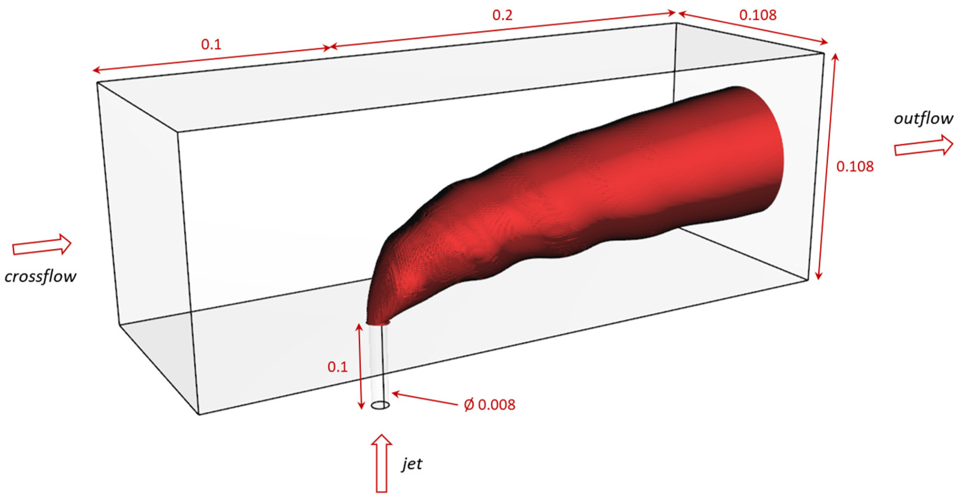
Considered experimental results and relevant setup have been previously described in [14,15]. Results have been obtained using the particle image velocimetry (PIV)/laser-induced fluorescence (LIF) methodology. The test setup consisted of a rectangular channel with a square cross section and a pipe. The pipe was mounted flush with the wall thus creating a round jet entrance. Diameter of the jet inlet equals $D=8\times {10}^{-3}\mathrm{m}$. Crossflow entrance side equals $a=0.108\mathrm{m}$. At the crossflow inlet, velocity is $9.08\mathrm{m}/\mathrm{s}$ hence the Reynolds number is $6.2\times {10}^4$. Velocity at the jet inlet is $37.72\mathrm{m}/\mathrm{s}$ with $Re=1.9\times {10}^4$. The velocity ratio equals $R=\left({\rho }_j{U}_j^2\right)/\left({\rho }_c{U}_c^2\right)=4.15$, where $\rho$ and U are respective densities and velocities. Additional information on the experimental setup and specifics can be found in the original paper [14].

2.2. Numerical Setup

Numerical simulations have been conducted in OpenFOAM [25]. A simplified computational domain has been used in all test cases [15]. An overview of the computational domain and relevant dimensions in meters has been given in Figure 1. All henceforth considered numerical grids are hexahedral.

At the crossflow and jet inlet, appropriate velocities are prescribed. Remaining patches, except for the outlet, are fixed walls. Value of the dimensionless wall distance, $y^{+}$, is below 4.52 in all test cases. According to [26], since this is a global maximum, design should be adequate as the first cell is within the viscous sublayer. Invariability of the first cell thickness in all AMR tests is ensured by excluding the relevant part of the domain from the refinement. Appropriate wall treatment is used for all considered turbulence models with blending enabled for turbulent viscosity through the employed nutUBlendedWallFunction boundary condition [27]. The considered fluid is air with a constant density and kinematic viscosity of $1.57\times {10}^{-5}{\mathrm{m}}^2/\mathrm{s}$. Turbulent mixing is assessed based on the concentration of the passive scalar, c, which is governed by the advection–diffusion equation

$$\frac{\partial c}{\partial t}=D_t{\nabla }^{2}c-\mathit{u}\nabla c$$

(1)

where t is time, $D_t$ turbulent diffusivity and $\mathit{u}$ velocity. The aforementioned transport equation as well as its steady variant are integrated in appropriate incompressible solvers. Value of the Schmidt number, unless stated otherwise, is $S{c}_t=0.9$. Influence of the molecular diffusion was neglected.

Employed numerical schemes are second-order accurate; implicit, second-order scheme is employed for time, Gamma01 scheme for transport equation, while limitedLinearV and limitedLinear schemes are used for remaining terms. Transient simulations lasted $0.5\mathrm{s}$ with the Courant number limited to $Co\le C{o}_{max}=0.9$. Averaging is conducted on the final $20\%$ of the simulation i.e., $0.1\mathrm{s}$. Convergence criteria is set to ${10}^{-5}$. Steady simulations adhere to the same guidelines, with the iteration limit set at $3\times {10}^4$.

Three RANS turbulence models have been considered: $k-ϵ$, $k-\omega$ TNT and $k-\omega$ SST. According to [14], two-equation $k-ϵ$ model [28] produces underwhelming results, however, since it is still commonly used, it is included in the assessments. $k-\omega$ TNT model is a modification of the Wilcox’s $k-\omega$ model and introduces additional constraints and new diffusion coefficients, thus eliminating the freestream dependency of the original model [29]. $k-\omega$ SST is nowadays used as a universal turbulence model mainly due to its flexibility; the model freely switches from $k-ϵ$ in the freestream to $k-\omega$ formulation near the walls, thus, mitigating the deficiencies of both models [30]. Furthermore, the SST model has been previously used to assess the turbulent mixing [15] and is thus an excellent starting point to comparatively evaluate the adaptive mesh refinement approach.

The adaptive mesh refinement employed in this study integrates three different conditions that ultimately govern the mesh generation. Initially, allowed refinement zones are defined within the domain so that, despite the inevitable push towards further refinement near the walls, cells in the boundary layer remain intact. This serves two purposes: it ensures equivalence at the wall between innately different grids while maintaining the smallest cell spacing and hence limiting the variable time-stepping due to enforced Courant value. Turbulence kinetic energy, k, serves as an intermediary refinement condition; it is used to pre-refine a zone. Cells in which $l_k\le k\le u_k$ are refined in order to smoothen the transition from coarse towards finer regions of the mesh. Upper bound, $u_k$, is an arbitrarily large number whereas $l_k=0.4$ for the coarsest mesh and is subsequently scaled down by a factor of 2 in each finer grid. Finally, concentration of the passive scalar, c, controls the fine refinement. Given that the results for a scalar transport problem are typically considered for $c=0.01$, bounds for refinement are set $0.0065\le c\le 0.012$. These bounds are similarly altered; each finer grid has its lower bound decreased by $5\times {10}^{-4}$ and higher bound increased by $6\times {10}^{-3}$, thus widening the zone of refinement. Refinement level i.e., maximum number of allowed cell subdivisions, has been capped at 2.

2.3. Testing Environment and Methodology

The test system is an Intel Xeon E5-2690v3 based cluster. Each cluster node has 24 physical cores and $64\mathrm{GB}$ of RAM. Unless otherwise noted, 2 nodes are used exclusively with hyperthreading disabled. Scaling tests rely on the same per-node resource distribution and simply utilize multiple nodes. Communication is facilitated by the Infiniband FDR link with a throughput of $51\mathrm{Gb}/\mathrm{s}$.

Assessments are made using the OpenFOAM v2012 with Infiniband enabled OpenMPI 4.0.3. The employed adaptive mesh refinement with load balancing is an adapted port of the code introduced in [2]. Custom solvers based on simpleFoam and pimpleFoam are also created. These integrate an additional transport equation and address other conflicts/issues. Furthermore, code for the $k-\omega$ TNT variant by Fürst [31] is used.

Initially, coarse, medium and fine grids have been created. Based on the GCI results, appropriate mesh has been chosen and subjected to a series of evaluations. Several aspects have been tested; difference between steady state and transient results, influence of the Schmidt number, Courant number and overall scaling for a chosen grid. Subsequently, AMR grids have been assessed with varying refinement approaches so as to determine the most appropriate setup for comparison with previous results. The initial AMR grid is a variant of the coarse grid unrefined by a factor of $1.3$. The boundary layer has been kept intact.

Results pertaining to the computational efficiency are three-run averages. Reported average timestep and memory use represent the average values during the final $20\%$ of the simulation, analogously to the previously noted averaging. Certain test cases necessitated the increase in the number of outer loops in order to ensure computational stability. These modifications are indicated.

3. Results and Discussion

3.1. Grid Convergence

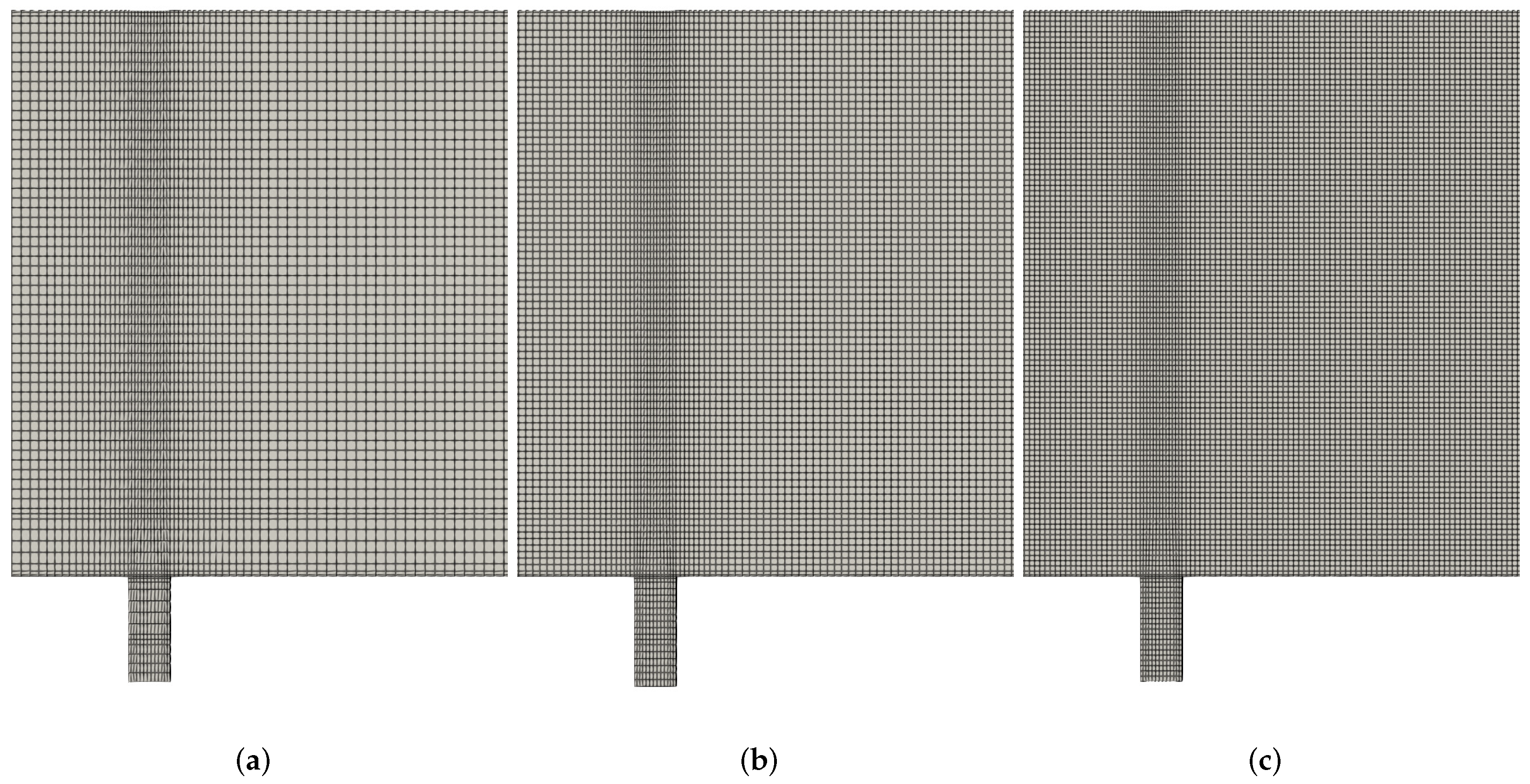
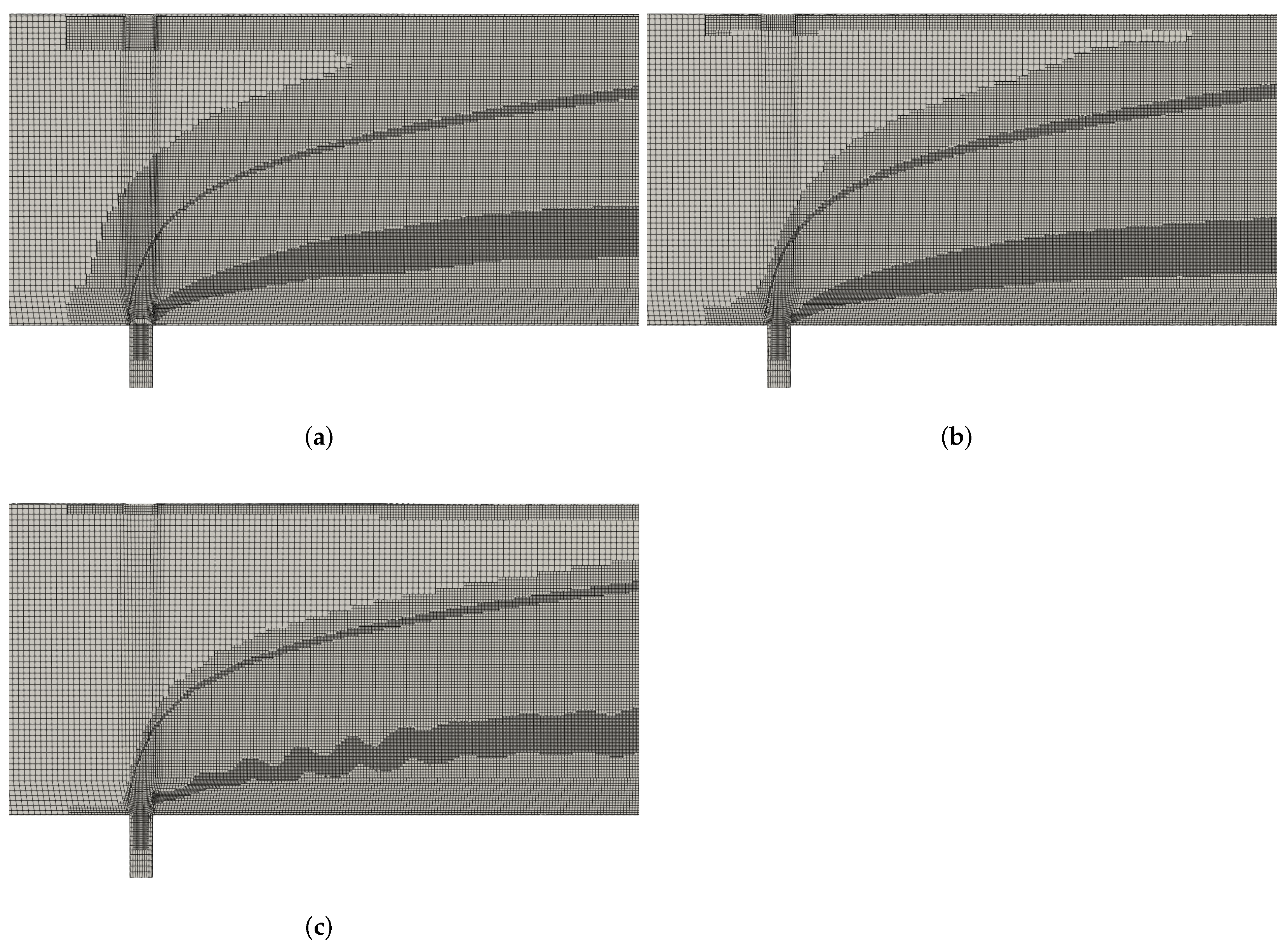
A grid convergence study has been conducted for the conventional mesh generation approach. Three sets of grids have been generated, namely coarse, medium and fine. Grids have approximately $7.2\times {10}^5$, $1.6\times {10}^6$ and $3.7\times {10}^6$ cells, respectively. A fragment of the computational domain near the jet centerline for each grid is given in Figure 2. The first cell is within the viscous sublayer for all cases. The downstream section of the computational domain in which the interaction occurs is resolved with $N_x=198$, $N_y=111$ and $N_z=109$ grid cells for the fine grid. Grid convergence index (GCI) was calculated for three considered locations downstream of the jet centerline [32]. Values presented in the

Table 1. Grid details and GCI for the conventional approach. Assessment is made at three locations downstream of the jet centerline for the passive scalar c.

Mesh	Cells	Ratio	$\mathit{x}/\mathit{D}=0.4$		$\mathit{x}/\mathit{D}=1.2$		$\mathit{x}/\mathit{D}=2.0$
	n	r	e [%]	GCI [%]	e [%]	GCI [%]	e [%]	GCI [%]
Coarse	$7.179\times {10}^5$	-	-	-	-	-	-	-
Medium	$1.638\times {10}^6$	1.3	3.419	0.359	13.900	9.157	10.762	0.424
Fine	$3.695\times {10}^6$	1.3	0.266	0.022	5.039	3.320	0.330	0.013

support the conclusion that the attained results are in the asymptotic range of convergence i.e., $GC{I}_{m,f}/(r^p\times GC{I}_{c,m})>0.95$ for all cases. Consequently, fine grid has been chosen for further assessments.

3.2. Conventional Approach

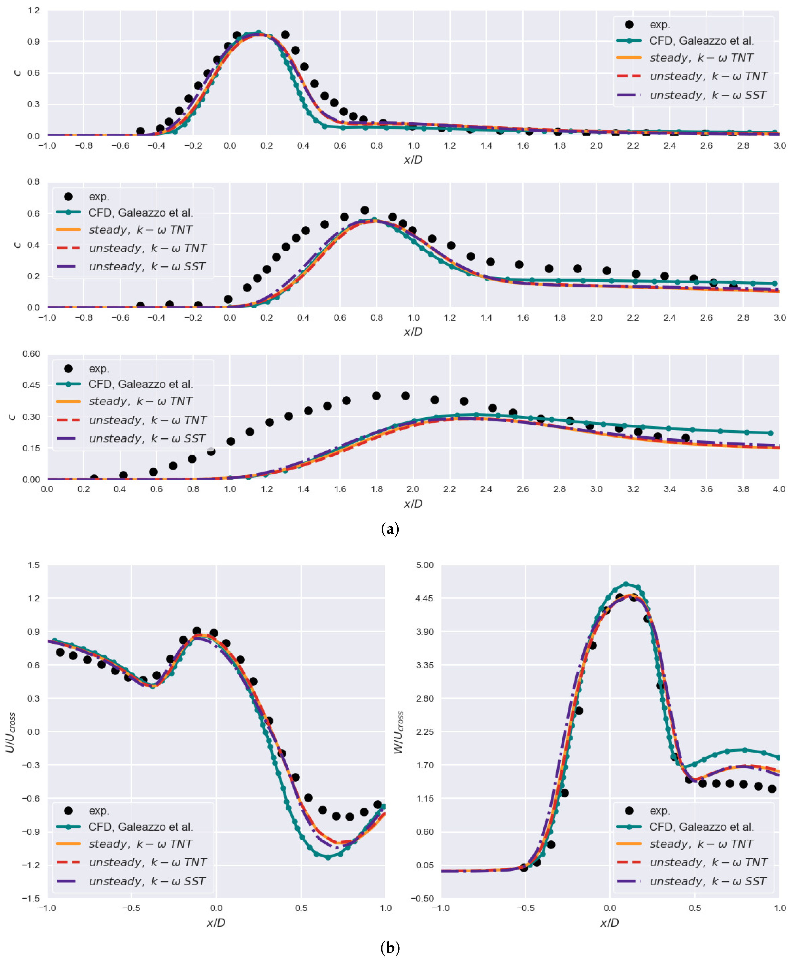
Multiple setups and simulation parameters were assessed in order to determine the appropriate settings for future AMR simulations. Steady state and transient simulations have been conducted using the $k-\omega$ TNT model. Additionally, transient simulation using the $k-\omega$ SST model has been conducted. Obtained results are compared to experimental results and RANS results calculated using the SST model and presented in [15]. Comparison is given in Figure 3.

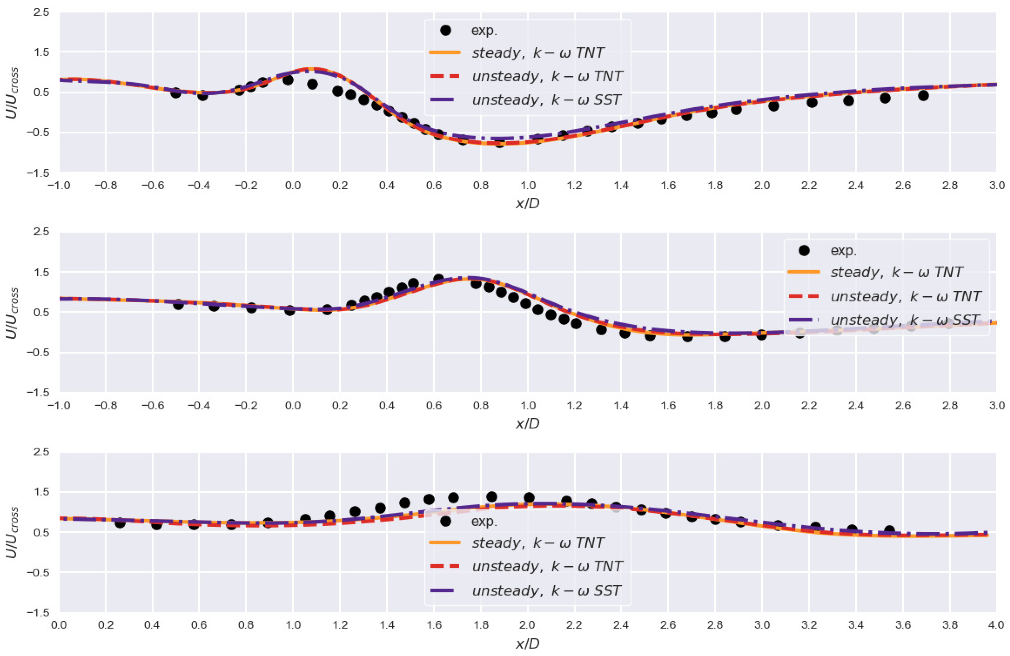
Overall, presented results match the experimental curve slightly better than the RANS results from [15]. This is true for steady and transient results. At $z/D=3$, downstream of the point $x/D=1.4$, scalar predictions are consistent but slightly worse. Still, for $z/D=4.5$, experimental trendline is better matched. Mean velocity profiles, $U/U_{cross}$ and $W/U_{cross}$, show a better trend as well. Mean values of passive scalar and velocity for steady and transient cases are virtually indistinguishable. This can be partially attributed to averaging conducted in order to report the results. Further validation is conducted for the velocity component $U/U_{cross}$. Similarly to scalar concentration, values are assessed at different $z/D$ sections. Results are given in Figure 4.

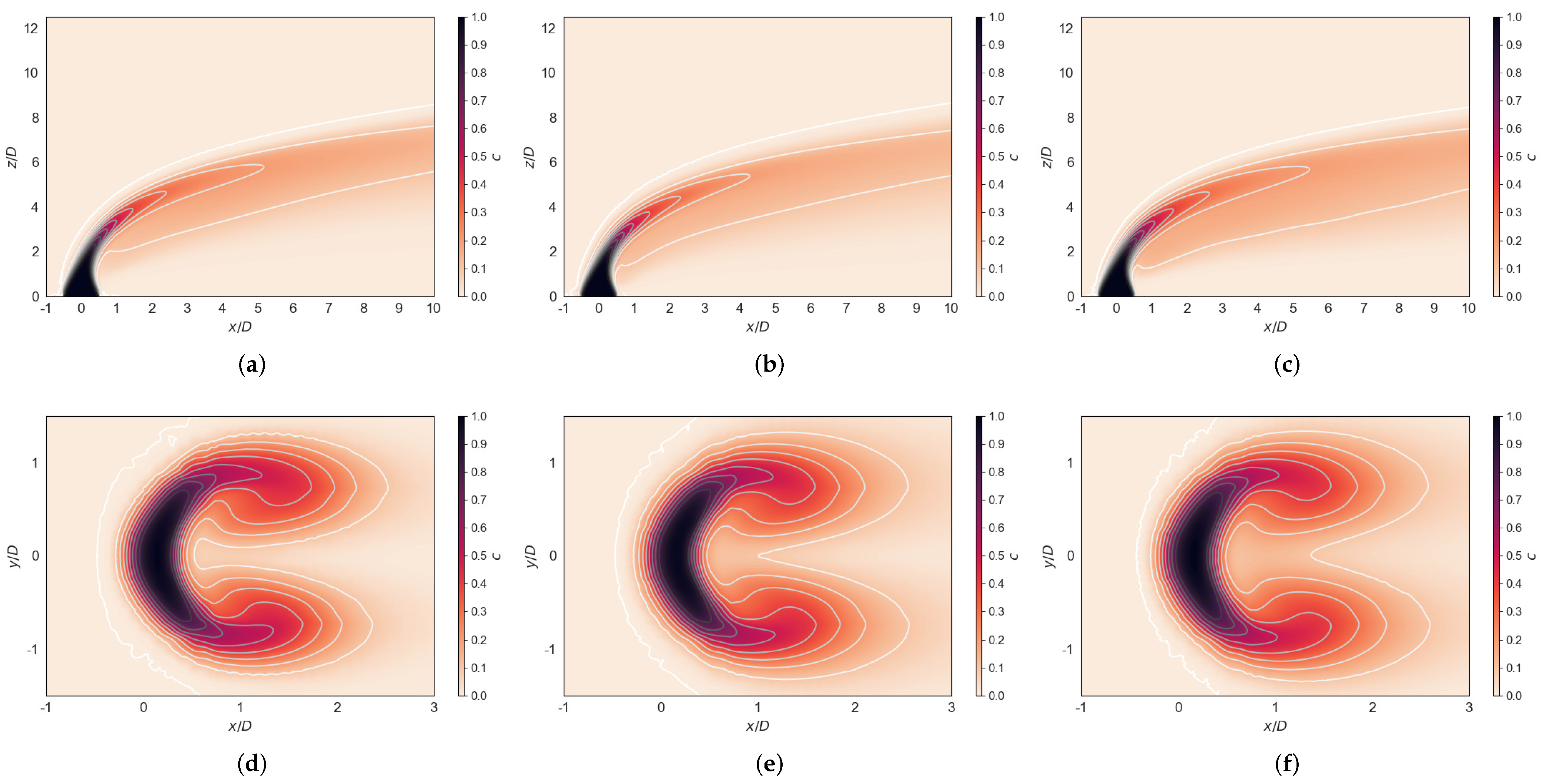
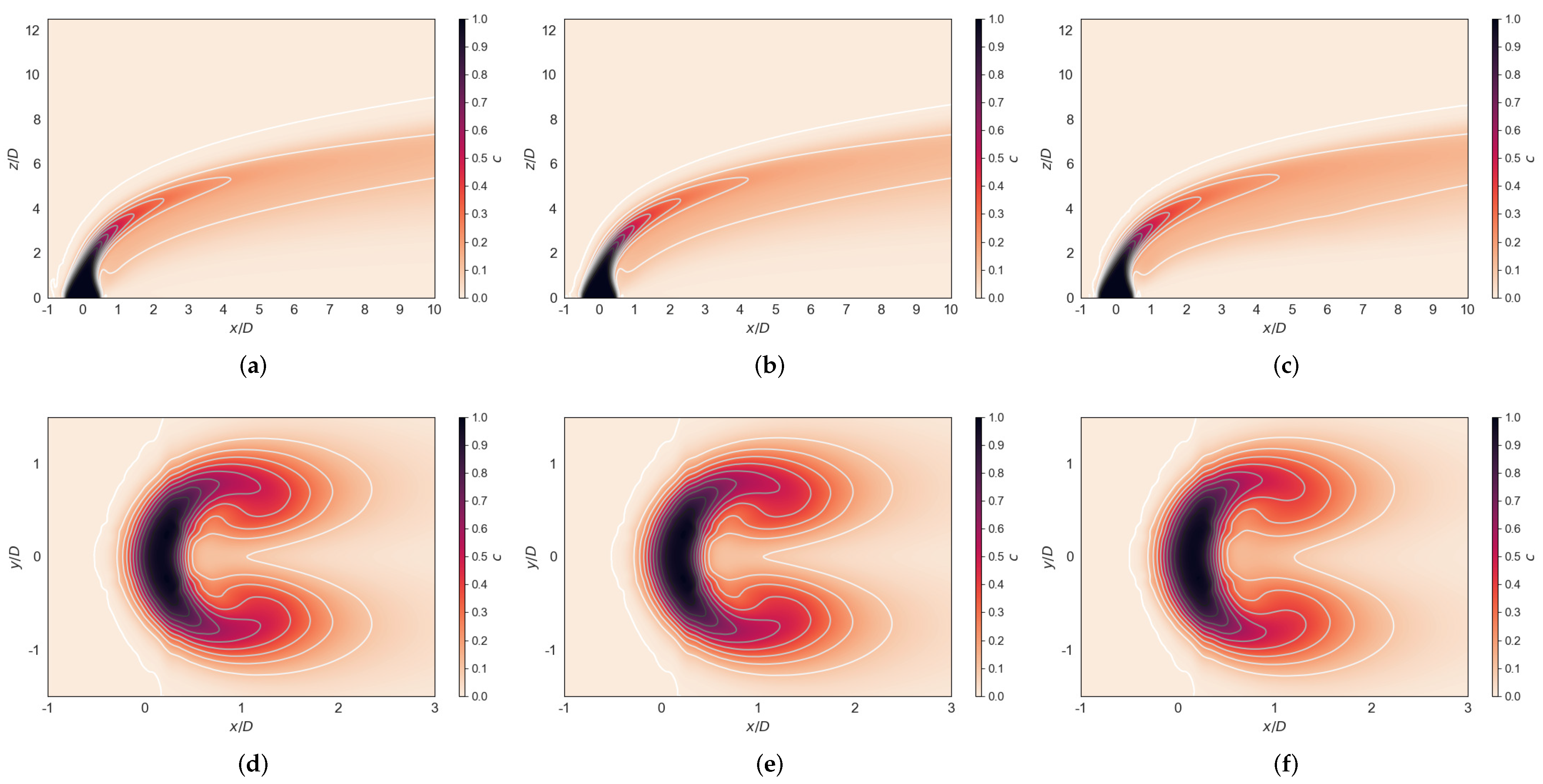
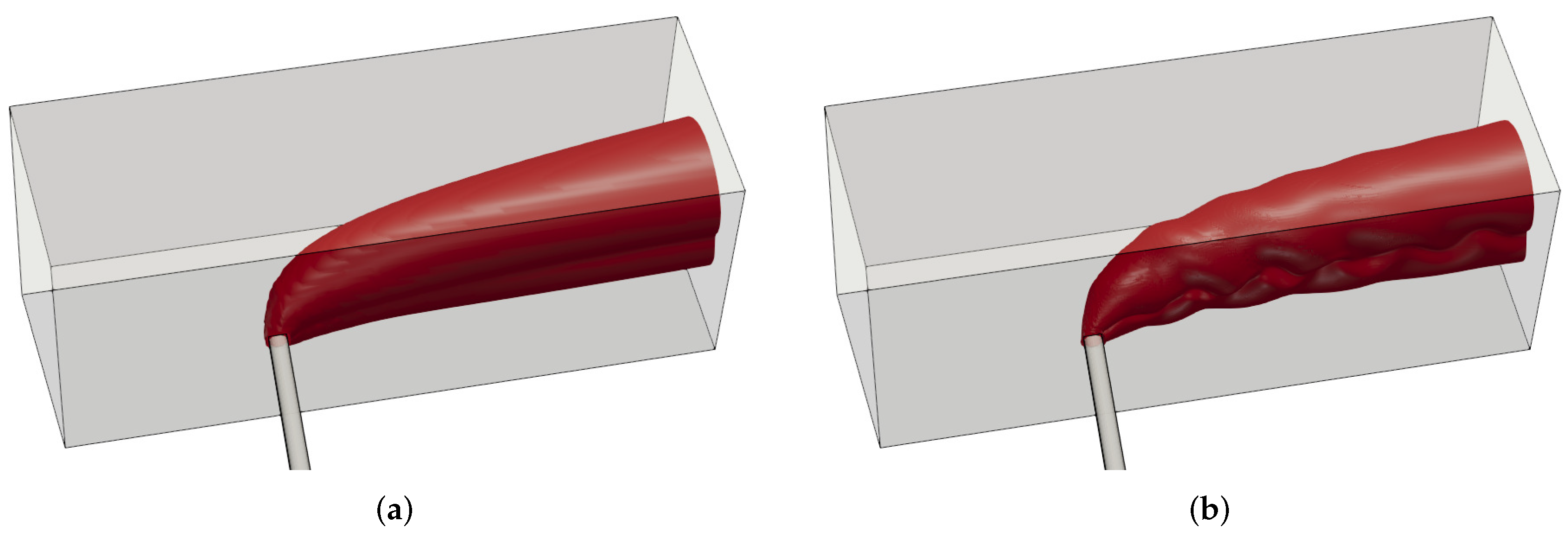
Based on Figure 4, velocity profile is reasonably reconstructed. There are, however, some notable discrepancies at $z/D=1.5$, $x/D=0.2$. Differences can be attributed to employed turbulence models and simplifications (domain simplification and missing inlet profiles). Two-dimensional plots of the scalar c at $y/D=0$ and $z/D=1.5$ are shown in Figure 5. The shape of the jet varies slightly for considered cases. Notably, TNT and SST model yield different inner shapes of the jet with slightly wider lower jet shear-layer obtained when using the SST model. Steady simulation delivers a moderately attenuated concentration distribution. In general, coherent structures are poorly predicted, particularly for the steady case. Transient simulations produce a distinguishable counter-rotating vortex pair. Results are as expected and similar to [15].

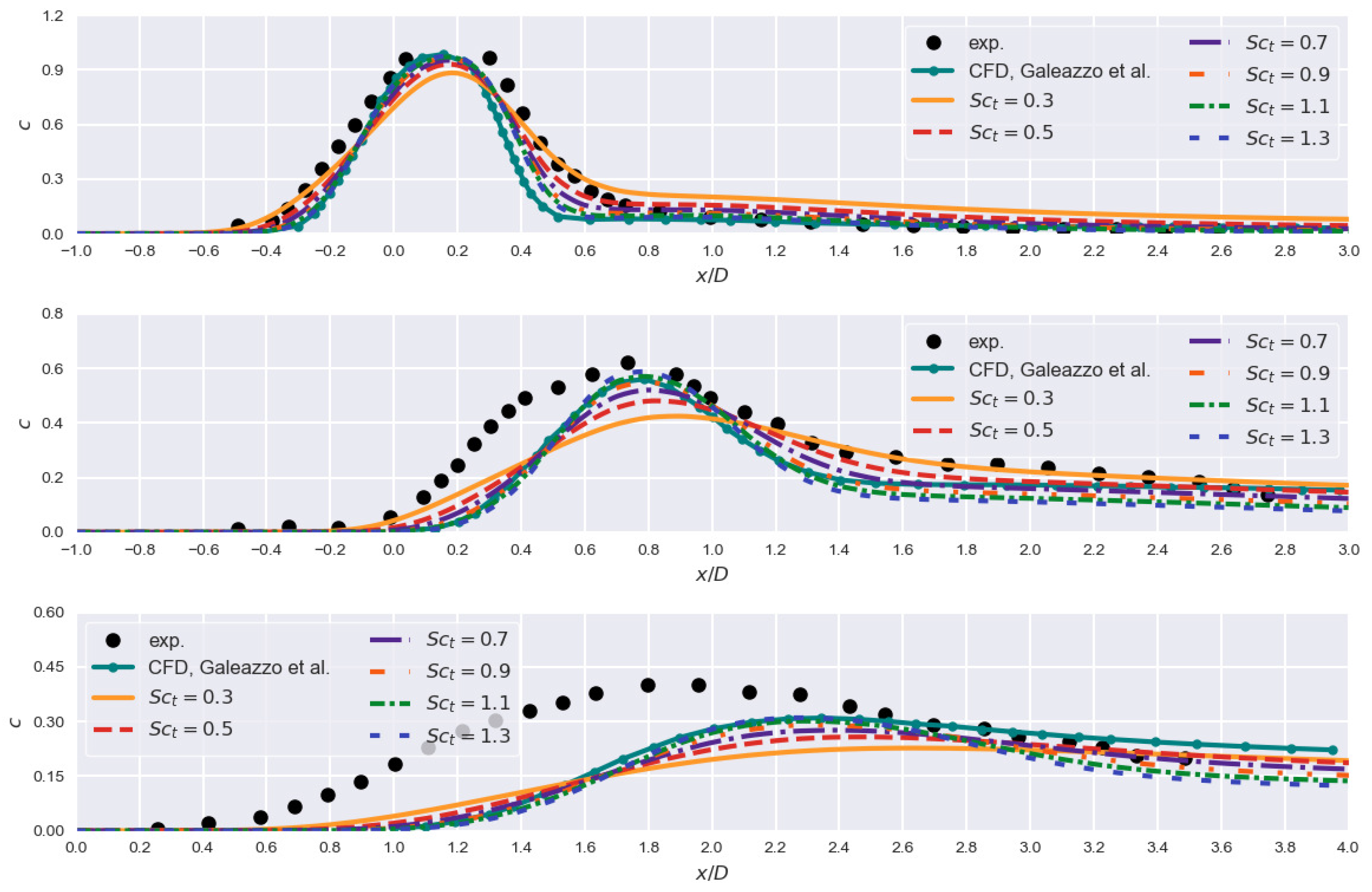
Several aspects of the current setup have been additionally assessed. Value of the turbulent Schmidt number, $S{c}_t=0.9$, is commonly suggested for RANS simulations [15,18,33]. Often, however, for specific turbulence models and depending on the problem, this value is modified. This aspect has therefore been considered and results for a range $0.3\le S{c}_t\le 1.3$ are presented in Appendix A, Figure A1. It is evident that satisfactory results are obtained for $S{c}_t=0.9$. Higher values are able to conform to peaks, but are lacking for the majority of the relevant region. Lower values on the other hand produce more sensible results but are inadequate when assessing concentration peaks. Utilized $S{c}_t$ is hence an appropriate choice and has been thus kept throughout.

Courant number of $C{o}_{max}=1$ is commonly used as a strict guideline to ensure the numerical stability for explicit and semi-implicit schemes. Since implicit second-order scheme is employed, aforementioned stability requirement is not necessary. As computational efficiency is a key aspect of this study, by increasing the Courant value and consequently the time step, overall computational time might be reduced. This approach, however, must attain the same levels of accuracy i.e., physics of the problem must be resolved. Figure A2 suggests that the change in Courant value does not affect the accuracy of the result; however, in order to ensure numerical stability, number of outer loops had to be increased, $n_{loops}=50$, which led to a significant increase in computational time, as is demonstrated by

Table A1. Performance on the fine grid for different CFL values. Assessment is made for the $k-\omega$ TNT model. Presented values are three-run averages. A total of 48 cores are used for all tests. Due to numerical instabilities, the number of outer loops had to be increased ($n_{loops}=50$) for $C{o}_{max}>0.9$.

CFL	0.9	1.5	3	5	10
Cells, n	3,695,236
Total time, t [s]	61,183	314,339	172,683	105,603	53,854
Avg. timestep, $t_{ts}$ [s]	1.010	8.381	9.743	9.863	9.790
RAM, m [GB]	9.754	11.190	10.345	9.937	9.556

. Accordingly, initial choice of the Courant number, $C{o}_{max}=0.9$, has been kept for all cases, since for $C{o}_{max}=10$ there is only a $13\%$ reduction in computational time.

3.3. Adaptive Mesh Refinement

Adaptive mesh refinement enables the creation of dynamically changing grids based on specific condition(s). The methodology is not novel, yet it is not commonly utilized. This is partially due to inherent variability of the numerical grids and consequently questionable accuracy of the results. Key aspects of the AMR process is now discussed.

Typically, a scalar value or phase fraction are used to refine the mesh in the zone of interest. It is questionable whether this is the most appropriate choice, namely for cases where physics of the problem can cause abrupt changes in mesh refinement levels. These changes contribute to the numerical diffusion and can hence impact the final result. Additionally, for more complex models, i.e., LES, refinement jumps and unrefined zones will govern which eddies are to be resolved. Still, AMR shows great potential and with proper use can be an acceptable approach even for complex LES simulations, where reduction in the computational requirements can lead to significant savings.

In accordance with the previous argument and as noted is Section 2.2, turbulence kinetic energy has been adopted in this study as an additional refinement condition that ensures slower transition between refinement levels. This effect can be clearly seen in Figure 6. It is important to note that this significantly increases the overall mesh size, but based on our findings, is an acceptable trade off.

Finally, stability of the numerical mesh should be a key consideration when using AMR. Although intuitively one could say that AMR will generate adequate grids as it is governed by the flow, issue arises when modeling the flow near the wall. The problem is twofold; when using turbulence models that rely on wall functions, excessive refinement in near-wall regions will lead to a change in first layer thickness thus altering the $y^{+}$ value and consequently will impact the calculations near the wall. Furthermore, additional refinement of boundary layer cells, which typically are the smallest cells in the domain, will lead to a notable change in time-stepping in order to maintain the CFL value. Presented problem, however, can be addressed. By limiting the regions of refinement to a zone which excludes the boundary layer, near-wall immutability can be achieved.

Unrefined preliminary grid employed for AMR in this study contained approximately $5.3\times {10}^5$ cells. The initial grid has iteratively been transformed according to methodology presented in Section 2.2. Results of the mesh refinement are presented in Figure 6.

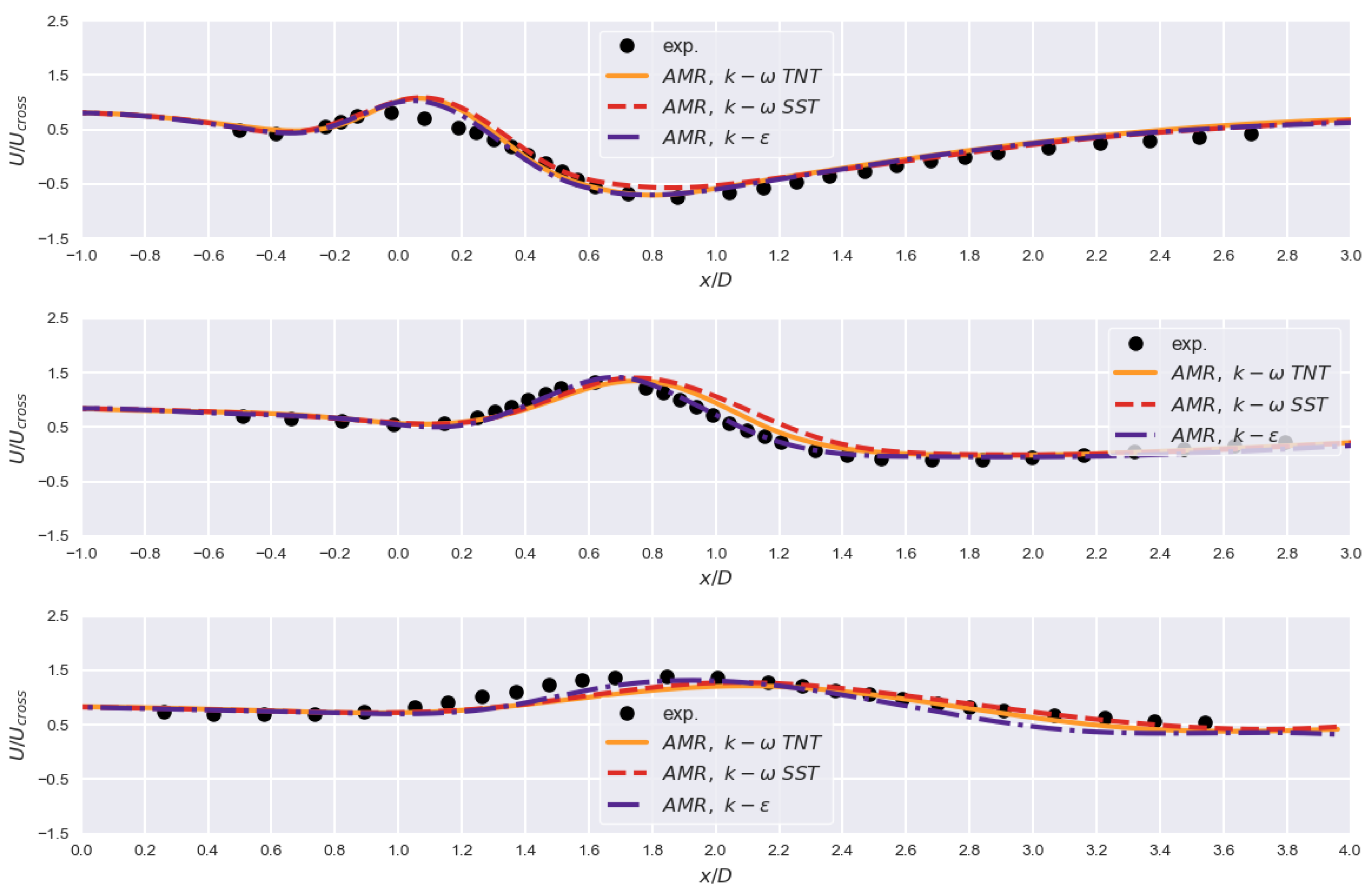
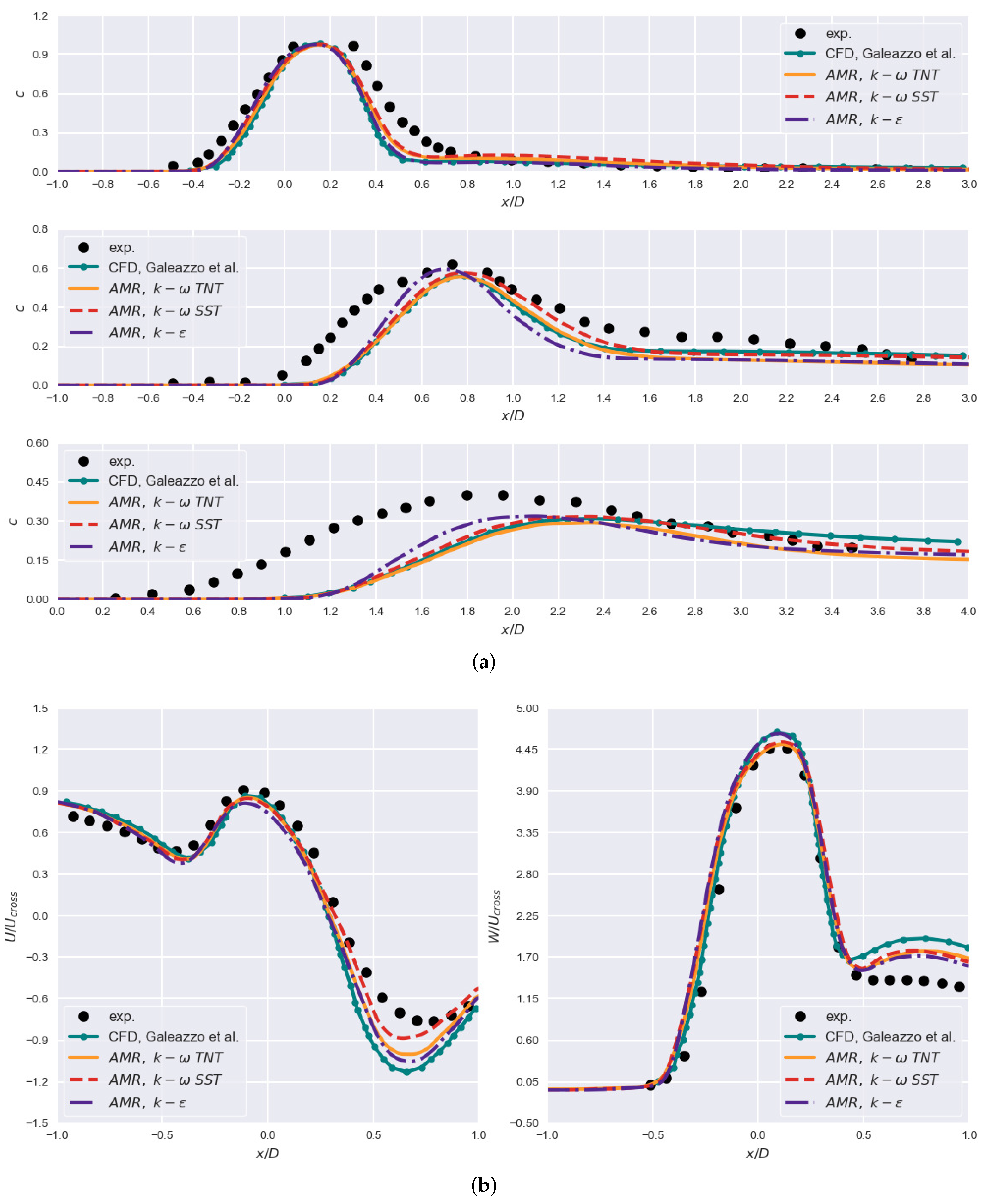
Applicability for the presented problem is henceforth assessed. Figure 7 demonstrates the agreement with the experiment for scalar c and profiles of mean velocity components when the mesh size is similar to the fine grid. At $z/D=1.5$, results mostly match the numerical results from [15] and previously noted results on the fine grid. Despite comparative equivalence, all RANS cases are unable to reproduce experimental results. The $k-ϵ$ model shows a deviation from the trend at $z/D=3$, downstream of point $x/D=0.8$. Although similar behavior is reported, current results are an obvious improvement. Similarly, at $z/D=4.5$, a minor variation can be observed. $k-\omega$ SST model produced convincing results throughout, followed by the TNT model. Rationale for this can be found in profiles of mean velocity where for $U/U_{cross}$ SST model approaches experimental results, surpassing the results on the fine grid. Results for the TNT model are similar to those on the fine grid. It is evident that the discrepancies are governed by resulting velocity fields i.e., are caused by the turbulence models.

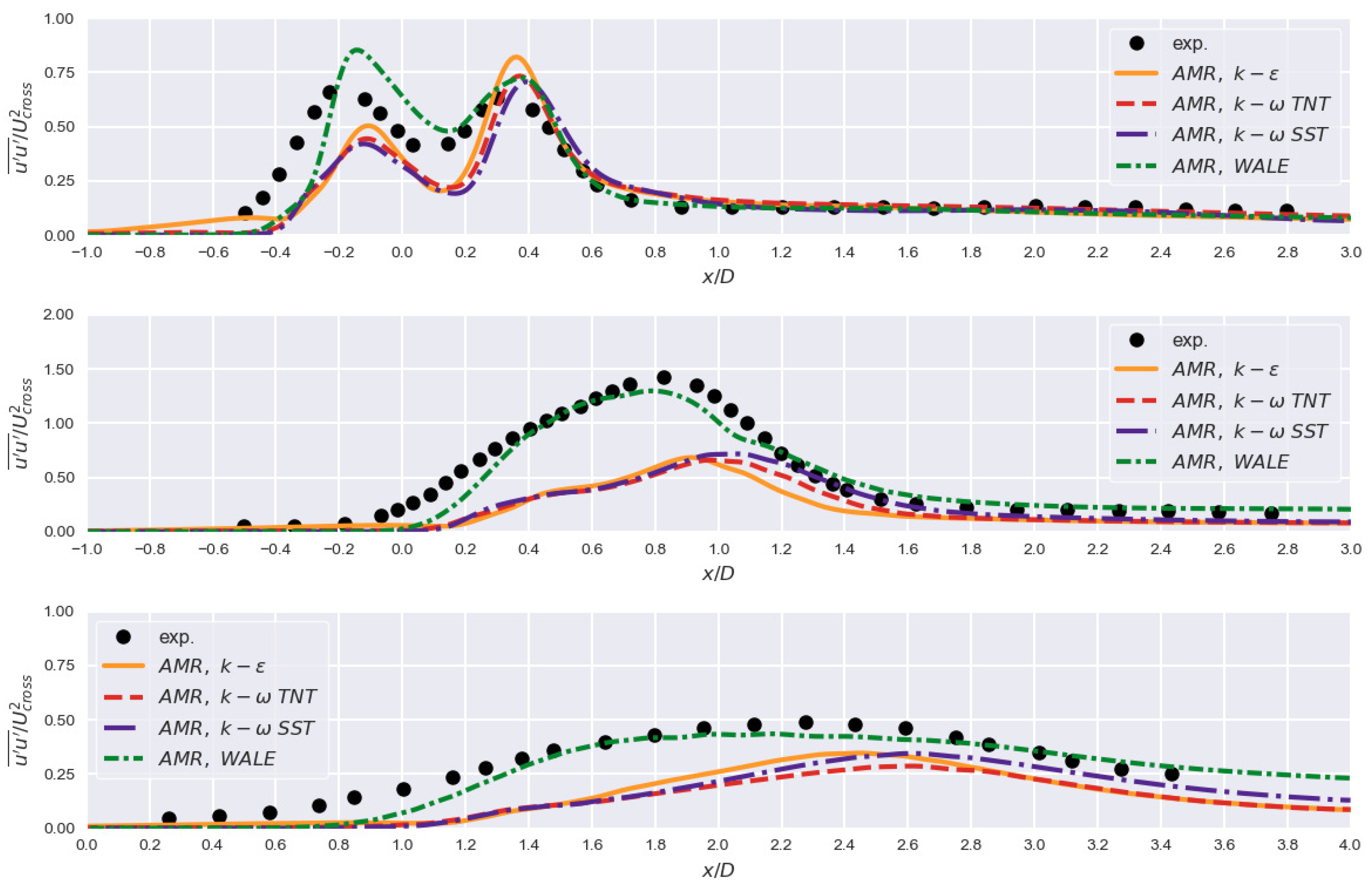
Figure 8 further underscores turbulence-model-associated discrepancies for velocity component $U/U_{cross}$. It is interesting to note that at $z/D=1.5$ and $z/D=3$, the $k-ϵ$ model seemingly surpasses other models; however, for $z/D=4.5$ it drops off, which manifests as a variation in the scalar concentration at that section. $k-\omega$ variants, for the most part, produce similar values. Overall, results are comparable to results on conventional grids.

Two-dimensional plots of scalar concentration presented in Figure 9 show good agreement with the results for the fine grid (Figure 5). Results for $y/D=0$ demonstrate a strong and amplified downstream trend. This is particularly true for $k-\omega$ variants. The SST model consistently assumes, based on values of c, broadest mixing region. For $z/D=1.5$, distribution zones of c are slightly enlarged when compared to Figure 5. The overall accuracy is satisfactory. Inability to fully reconstruct the experiment is typical for RANS models; they tend to provide acceptable mean values but are unable to fully resolve flow specifics.

3.4. Computational Efficiency and Load Balancing

One of the major hindrances when using AMR is associated performance deterioration. Typically, a complex OpenFOAM case on a system with multiple cores (hereinafter processors) is executed in parallel and decomposed. Each of the processors is assigned a specific subdomain and data are exchanged only for shared faces. The described approach is appropriate for static, immutable grids; however, when using adaptive refinement, regions assigned to a specific processor can be, depending on the refinement methodology, significantly altered, both topologically and in terms of the overall cell count. Once a processor is assigned a significantly disproportional number of cells or is at maximum utilization, the overall computational efficiency will drop as the remaining processors are forced to wait. In order to address this, load balancing is introduced. Methodology behind the load balancing is rather simple: software tracks the disbalance between the processor loads and redistributes the mesh accordingly.

Table 2. Computational efficiency on fine grid and when using the AMR approach without load balancing.

Case	Fine	AMR	AMR
	$\mathit{k}-\mathit{\omega }$ TNT	$\mathit{k}-\mathit{\omega }$ TNT	$\mathit{k}-\mathit{\omega }$ SST
Cells, n	3,695,236	3,770,395	2,850,847
Total time, t [s]	61,183	104,631	123,465
Avg. timestep, $t_{ts}$ [s]	1.010	2.364	2.463
RAM, m [GB]	9.754	17.108	15.080

demonstrates the main problem of using AMR without load balancing; computational times for similarly sized grids are significantly longer (up to $200\%$). Cell size discrepancy for $k-\omega$ TNT and SST models when using the AMR approach is a direct consequence of the innate differences between the turbulence models; for identical setups, calculated values of scalar c and kinetic energy k govern the refinement of the primary grid. Still, despite that, the SST model has the longest computational time.

With load balancing, computational times can be, on average, reduced by more than $45\%$, as is shown in

Table 3. Impact of load balancing on computational efficiency when using AMR.

Case	Balancing Disabled			Balancing Enabled
	$\mathit{k}-\mathit{ϵ}$	TNT	SST	$\mathit{k}-\mathit{ϵ}$	TNT	SST
Cells, n	3,743,793	3,770,395	2,850,847	3,746,180	3,770,836	2,851,503
Total time, t [s]	548,479	104,631	123,465	282,719	57,127	66,171
Avg. timestep, $t_{ts}$ [s]	24.807	2.364	2.463	12.636	1.296	1.333
RAM, m [GB]	9.462	17.108	15.080	14.876	13.685	12.314

. Since there is no observable change in the overall accuracy of the results, attained savings should encourage the use of the AMR. Additional information pertaining to the performance of the AMR methodology is included in the Appendix B. Furthermore, comparison of computational times on similarly sized grids does not take into consideration the main advantage of the AMR methodology; the given problem can be resolved by utilizing a less computationally demanding case (i.e., numerical grid), since refinement is conducted only in relevant zones/region of interest.

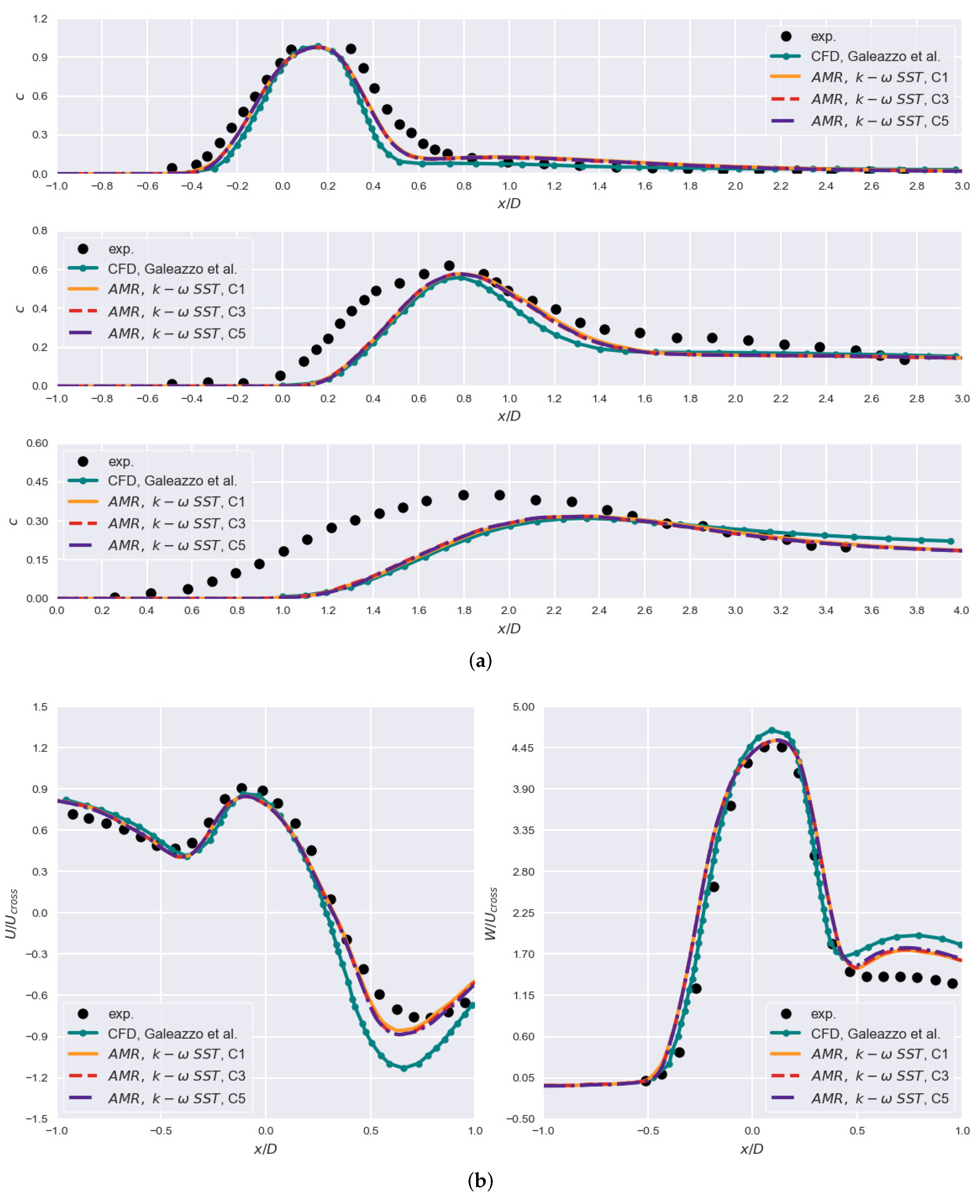
Aforementioned supposition is affirmed by results presented in Figure 10. Values of passive scalar c and velocity profile components are contrasted for three different cases with $1.6\times {10}^6$, $2.15\times {10}^6$ and $2.85\times {10}^6$ cells, respectively. As can be seen, even though there are slight variations for the coarsest case, it is evident that the results are mostly equivalent.

Thus far, noted AMR cases permitted refinement every 1000 iterations (timesteps) with load balancing conducted when the imbalance reaches $20\%$. Detailed results for all considered turbulence models and with regards to the load balancing are included in Appendix C (

Table A5. AMR generated grids when using the $k-ϵ$ model. Refinement frequency is set to 1000 timesteps. Load balancing is disabled. AMR specifics are defined in the manuscript. Presented values are three-run averages. A total of 48 cores are used for all tests. Due to numerical instabilities, the number of outer loops had to be increased ($n_{loops}=20$).

Cells, n	1,635,190	2,131,756	2,699,904	3,256,761	3,743,793	4,171,500
Total time, t [s]	213,972	293,283	416,898	492,013	548,479	610,740
Avg. timestep, $t_{ts}$ [s]	9.428	13.329	17.508	22.222	24.807	26.648
RAM, m [GB]	7.274	7.723	8.024	8.744	9.462	10.271

,

Table A6. Results for setup identical to Table A5 with load balancing enabled and performed when the imbalance reaches $20\%$.

Cells, n	1,674,068	2,160,666	2,682,159	3,256,502	3,746,180	4,182,035
Total time, t [s]	121,036	152,235	191,997	245,430	282,719	328,035
Avg. timestep, $t_{ts}$ [s]	5.326	7.003	8.752	10.991	12.636	14.474
RAM, m [GB]	10.048	10.929	12.780	13.915	14.876	16.068

,

Table A7. AMR generated grids when using the $k-\omega$ TNT model. Refinement frequency is set to 1000 timesteps. Load balancing is disabled. AMR specifics are defined in the manuscript. Presented values are three-run averages. A total of 48 cores are used for all tests.

Cells, n	1,648,562	2,153,262	2,567,886	3,139,800	3,770,395	4,568,486
Total time, t [s]	44,703	56,000	75,137	93,349	104,631	122,059
Avg. timestep, $t_{ts}$ [s]	1.014	1.196	1.696	2.098	2.364	2.673
RAM, m [GB]	9.736	11.674	13.106	15.321	17.108	18.757

,

Table A8. Results for setup identical to Table A7 with load balancing enabled and performed when the imbalance reaches $20\%$.

Cells, n	1,670,976	2,150,553	2,569,461	3,142,047	3,770,836	4,568,983
Total time, t [s]	23,683	29,469	37,496	46,964	57,127	69,733
Avg. timestep, $t_{ts}$ [s]	0.538	0.639	0.850	1.076	1.296	1.486
RAM, m [GB]	9.128	10.184	11.583	12.558	13.685	16.707

,

Table A9. AMR generated grids when using the $k-\omega$ SST model. Refinement frequency is set to 1000 timesteps. Load balancing is disabled. AMR specifics are defined in the manuscript. Presented values are three-run averages. A total of 48 cores are used for all tests.

Cells, n	1,593,696	1,890,216	2,149,496	2,445,512	2,850,847	4,127,374
Total time, t [s]	57,857	72,595	84,600	98,321	123,465	161,944
Avg. timestep, $t_{ts}$ [s]	1.180	1.471	1.728	2.009	2.463	3.030
RAM, m [GB]	10.093	11.268	12.305	13.363	15.080	18.380

and

Table A10. Results for setup identical to Table A9 with load balancing enabled and performed when the imbalance reaches $20\%$.

Cells, n	1,607,775	1,891,996	2,150,862	2,445,944	2,851,503	4,128,115
Total time, t [s]	31,972	39,160	42,714	50,833	66,171	89,405
Avg. timestep, $t_{ts}$ [s]	0.663	0.807	0.872	1.110	1.333	1.689
RAM, m [GB]	9.036	9.834	10.559	11.013	12.314	14.863

). Additionally, refinement frequency and imbalance level were assessed i.e., their influence on the computational efficiency. These results are included in

Table A11. Influence of the refinement frequency on the computational time. Setup is identical to Table A7 with load balancing enabled and performed when the imbalance reaches $5\%$.

Frequency	10	50	100	500	1000
Cells, n	3,793,285	3,788,252	3,775,575	3,768,449	3,773,790
Total time, t [s]	147,421	91,853	65,316	58,514	57,493
Avg. timestep, $t_{ts}$ [s]	2.595	1.562	1.438	1.315	1.306
RAM, m [GB]	16.164	15.697	14.702	15.162	13.985

,

Table A12. Influence of the refinement frequency on the computational time. Setup is identical to Table A7 with load balancing enabled and performed when the imbalance reaches $20\%$.

Frequency	10	50	100	500	1000
Cells, n	3,789,764	3,785,494	3,774,413	3,767,392	3,770,836
Total time, t [s]	149,921	105,332	68,027	58,432	57,127
Avg. timestep, $t_{ts}$ [s]	2.679	1.909	1.520	1.311	1.296
RAM, m [GB]	16.430	15.755	15.106	14.989	13.685

,

Table A13. Influence of the load balancing (imbalance adjustment) on the computational time. Setup is identical to Table A7 with refinement frequency set to 10 timesteps.

Imbalance	$2.5\%$	$5\%$	$10\%$	$20\%$	$40\%$
Cells, n	3,794,307	3,793,285	3,791,325	3,789,764	3,788,651
Total time, t [s]	128,477	147,421	142,727	149,921	146,456
Avg. timestep, $t_{ts}$ [s]	1.225	2.595	2.483	2.679	2.605
RAM, m [GB]	15.263	16.164	16.355	16.430	16.493

and

Table A14. Influence of the load balancing (imbalance adjustment) on the computational time. Setup is identical to Table A7 with refinement frequency set to 1000 timesteps.

Imbalance	$2.5\%$	$5\%$	$10\%$	$20\%$	$40\%$
Cells, n	3,777,773	3,773,790	3,772,957	3,770,836	3,770,892
Total time, t [s]	57,932	57,493	56,999	57,127	57,755
Avg. timestep, $t_{ts}$ [s]	1.333	1.306	1.291	1.296	1.311
RAM, m [GB]	14.234	13.985	13.981	13.685	13.577

. Results demonstrate that with the increase in refinement frequency, computational time is also increased. This is expected, since frequent refinement steps introduce non-computational delays which lengthen the overall computation and for cases without load balancing can quickly lead to a general slowdown. Although it might seem favorable to instigate the refinement step frequently, only for exceedingly time-varying (changing) cases this is pertinent. For common problems, mesh refinement will reach an equilibrium where refinement and unrefinement will largely cancel each other out whilst the mesh will remain mostly constant. It is also interesting to note that lower imbalance limits are favorable for frequent refinements. Overall, however, imbalance limits have little influence on the computational time as is shown in Table A13 and Table A14.

3.5. LES Considerations

The fundamental prerequisite for LES modeling is proper mesh resolution. Adaptive mesh refinement and inherent inconstancy of the grids make the assessment of the grid applicability impractical. This in itself is a lengthy topic outside of the scope of this paper and hence will not be further discussed here. It is important to note, however, that the predictions of coherent structures and the accuracy of results are directly related to the quality of the computational mesh (refinement) as scales smaller than the employed cell sizing cannot be resolved, rather they are modeled [34].

Numerical setup described in Section 2.2 is analogously used for the considered wall-adapting local eddy-viscosity (WALE) model [35]. WALE is adopted as it does not require damping in near-wall regions and should hence be more stable for use with AMR. limitedLinear01 1 and LUST schemes are used for c and U, respectively. Schmidt number $S{c}_t=1$ suggested in [15] is employed. Due to pressure instabilities, a constant number of outer loops, $n_{loops}=5$, is set. At the inlets, a synthetic eddy generator, turbulentDFSEMInlet is used. Necessary values of the Reynolds stress tensor, integral length scales and velocities at the inlets are obtained from SST simulations. Refinement is conducted with regards to the geometrical constraints (at least two cell layers near the walls are immutable) and Q-criterion. This was performed so that the zones containing vortices and vortex structures are properly captured. Number of cells is approximately $5.5\times {10}^6$. 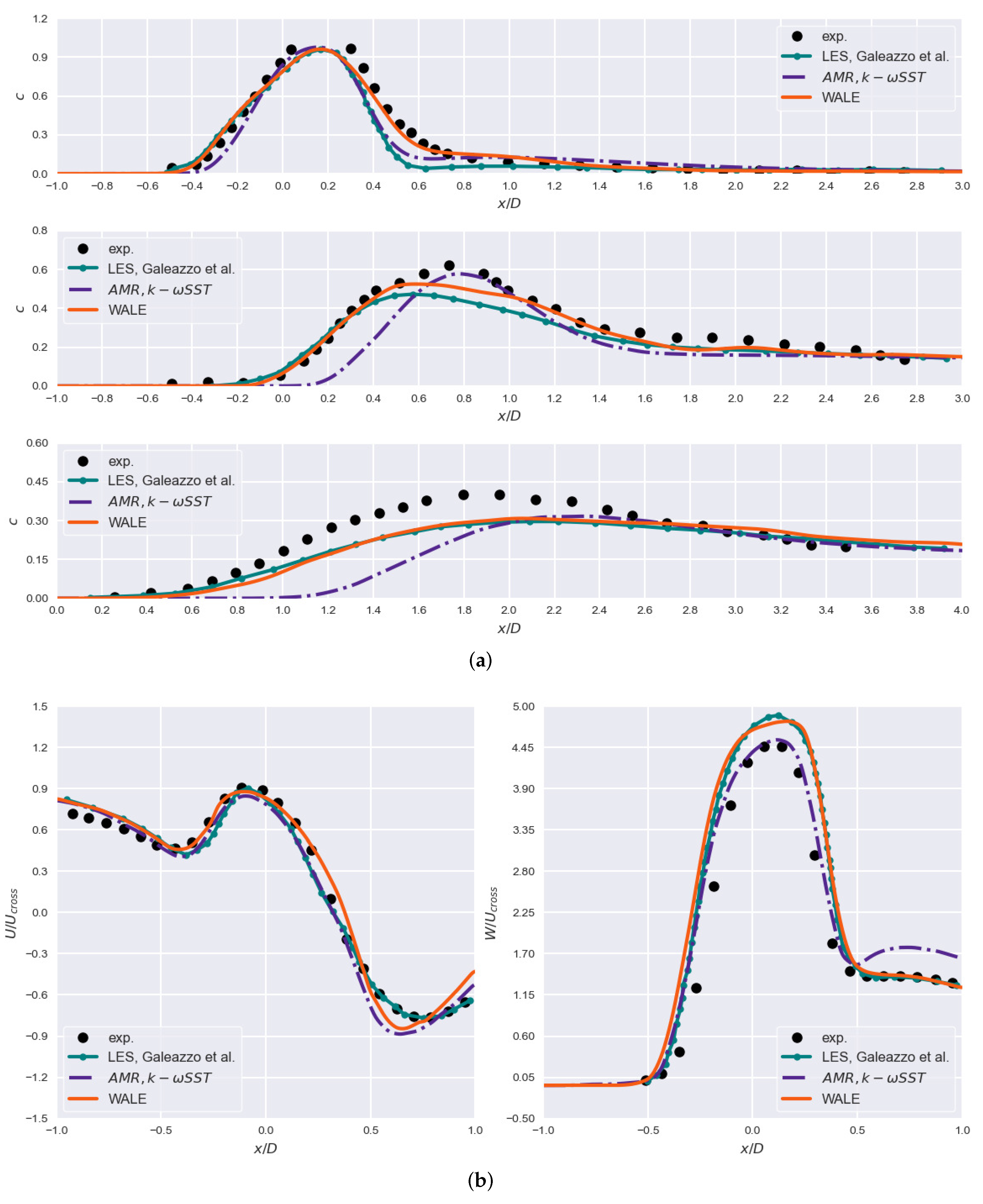Results for noted setup are presented in Figure 11.

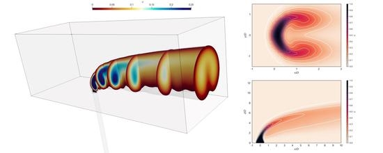
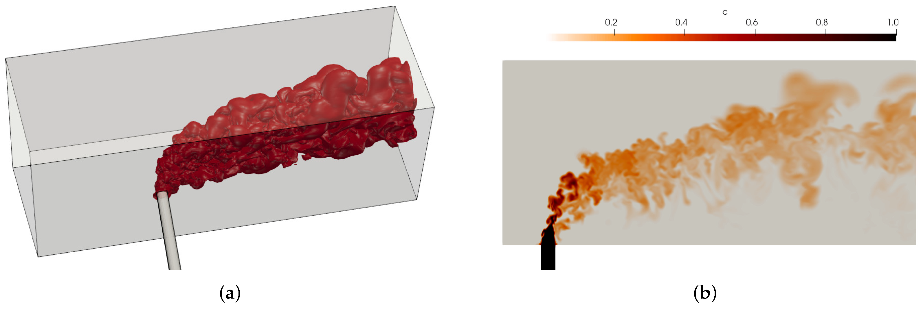
It is evident that the LES results are in better agreement with the experimental data. This is especially true for passive scalar at $z/D=3$ and $z/D=4.5$. For $z/D=1.5$ scalar distribution is nearly perfectly reconstructed. There are some discrepancies, however, namely for $U/U_{cross}$ downstream of $x/D=0.5$ and $W/U_{cross}$ near $x/D=0$. Although it is fair to assume that this is caused by the AMR, result similarity with other LES studies indicates that this might be a problem inherent to the LES modeling or missing experimental data. These disparities require further investigation. Nevertheless, it has been established that AMR and inherent computational savings related to load balancing provide the ability to accurately and efficiently assess the JIC problem. Additionally, the isosurface of scalar $c=0.01$ and its distribution at $y/D=0$ calculated using WALE model and AMR are given in Figure 12.

4. Conclusions

Adaptive mesh refinement and its applicability is a complex topic that requires extensive investigation. On the face of it, benefits of the approach are obvious and numerous; it allows for quick and accurate estimates in resource-constrained computational environments. However, as is the case with all techniques, there are some drawbacks and potential pitfalls which must be considered.

Use of AMR on non-HPC systems and systems with limited processing power as well as general use, which does not include problem parallelization, fails to uncover one of the main issues of the AMR natively included in OpenFOAM distributions which is load-associated performance deterioration. From a computational standpoint, this is a major hindrance to AMR use, namely for larger, complex and real-world problems.

This study tried to address and clarify key aspects of AMR use by analyzing a turbulent mixing problem of a jet in crossflow. Overall accuracy for a given problem is assessed and compared to experimental and previous numerical results. Additionally, load balancing, its parameters and significance are investigated and discussed.

Initially, conventional approach using RANS turbulence models to analyze turbulent mixing of a jet in crossflow was considered. Results showed good agreement with previous numerical studies. At worst, predicted scalar concentration differed by $c=0.1$ whereas velocity components $U/U_{cross}$ and $W/U_{cross}$ deviated by 0.5 and 0.3. These discrepancies, however, are an improvement as they lead to better agreement with the experimental data. Expanding on this, an unrefined coarse grid was employed for a series of AMR case studies for varying turbulence models and parameters. Results were encouraging and acceptable and showed the potential of the adaptive mesh refinement; even the coarsest considered cases were satisfactory. Differences between scalar concentrations were negligible (for best cases). Subsequently, emphasis was given to load balancing and its influence on computational time. When normalized by the cell count, considered AMR cases without load balancing exhibited up to $72\%$ longer computational times than conventionally defined problems. With the inclusion of load balancing, AMR cases completed in approximately $7\%$ less time. Based on our findings, load balancing can reduce AMR computational times by more than $50\%$. Furthermore, it has been shown that AMR cases can achieve accuracy similar to conventional methodology with significantly lower cell count, thus further reducing computational time. Key observations and suggestions will now be briefly noted:

• AMR is suitable for turbulent mixing problems. Accuracy is on par with the conventional approach.
• Use for complex problems with bounded regions of interest is desirable.
• AMR approach can be employed to generate problem-specific grids as opposed to generating grids using conventional methodology.
• In order to avoid abrupt changes in mesh refinement, multi-criteria approach is suggested.
• Ensuring immutability of the boundary layer is a key factor in maintaining computational efficiency. This should also ensure CFL stability.
• Refinement frequency is the principal parameter governing the computational effort in AMR. Frequent refinement steps are typically not necessary, at least for JIC problems and RANS. Accordingly, additional computational savings can be achieved.
• Load balancing is indispensable for complex problems; however, simpler problems can also benefit from it. Due to load balancing, computational times can be halved.