TAID-LCA: Segmentation Algorithm Based on Ternary Trees

Abstract

In this work, a statistical method for the segmentation of samples and/or populations is presented, which is based on a ternary tree structure. This approach overcomes known limitations of other segmentation methods such as CHAID, concerning the multivariate response and the non-symmetric relationship between explanatory and response variables. The multivariate response segmentation problem is handled through latent class models, while the factorial decomposition of the explanatory capability of variables is based on the Non-Symmetrical Correspondence Analysis. Stop criteria based on the CATANOVA index and impurity measures are proposed. A Simulated Annealing based post-pruning strategy is considered to avoid over-fitting relative to the training set and guarantee a better generalization capability for the method.

1. Introduction

Nowadays, segmentation methods, techniques, and algorithms are widely used in several scientific disciplines (such as Social Sciences, Health Sciences, Communication Sciences, among others), for identifying heterogeneous groups of subjects (In this work, we indistinctly use the words: subjects, items or records, to refer to the same concept: the objects to be segmented in groups. This is because of the diverse vocabulary generally used in several disciplines that provide different segmentation approaches, improvement methods, and evaluation strategies.), classified according to certain features, such as their opinion about some topics, their social-demographic profile, their consumption behavior, etc.

In a typical segmentation problem, a single response (target) variable and several explanatory variables are given. In this case, the problem is said to be univariate, and if more than one response variable is given, then the segmentation problem is said to be multivariate.

The CHAID method (Chi-square Automatic Interaction Detection (AID)), proposed by Kass [1] and based on the AID methods of Morgan and Sonquist [2], is a very popular exponent of the recursive segmentation trees methods see, e.g., [3,4]. Furthermore, its implementation is included in widely used statistical softwares such as STATISTICA [5] or SPSS [6]. In platform R see [7].

The Classification and Regression Trees (CART) methods, proposed by Breiman et al. [8] are also very popular and widely used in different domains of application.

These methods consider several explanatory variables and only one response variable. Nevertheless, many segmentation problems have a multivariate response nature. Repeating the analysis for each response variable involves, at least, a notable increment in the risk of Type I. Generally, such methods are based on the Chi-Squared test, but this test does not distinguish between the explanatory and the response role of a variable; it simply determines whether or not the variables are covariate.

Galindo-Villardón et al. [9] have proved that in certain circumstances, the CHAID method is not able to detect interactions; they stated that this is due to the marginal independence tests it is based on. They proposed an AID algorithm based on conditional rather than marginal independence tests and using conditional entropy measures to test conditional independence.

On the other hand, during a launch of the CHAID algorithm, categories of variables are collapsed see [1], but certain conditions should be fulfilled in order for this to be meaningful. In that sense, Avila [10] and Dorado-Díaz [11] have proved that such conditions are not verified in general.

Our alternative approach is based on the idea of using association coefficients, regarding the asymmetrical nature of data, [12]. In the case of multivariate response, the first step is to define a latent variable which summarizes the multivariate response. Furthermore, Siciliano and Mola [13] advise that the method should not only focus on the identification of variables for segmenting, but it should also identify which categories of each explicative variable are the ones with the best explanatory power for each response category.

Recently, [14] presented an important contribution QUEST algorithm that decreases uncertainty to compare with CHAID. Other research presents [15] the same algorithm to predict business behaviors with high precision. However, TAID (Tau Automatic Interaction Detection) gives another way to compare the information with the same accuracy. This proposal, unlike those discussed above, is more robust since it considers models of latent classes in the response and segmentation criteria with significant categories, which makes the information relevant.

2. TAID-LCA Algorithm General Steps

We call our algorithm TAID-LCA, which stands for Tau Automatic Interaction Detection—Latent Class Analysis, due to the use of the Tau ($\tau$) index in the explanatory power (non-symmetrical) analysis (see Section 4.1), and the use of the Latent Class Analysis (LCA) to handle the multivariate response (see Section 3).

The input of the algorithm is a data set with explanatory and manifest variables. The manifest variables are the target ones (the ones to be explained), they give a rough characterization of the underlying latent classes of subjects. The output of the algorithm is a ternary tree, yielded from the recursive partition by the values of the explanatory variables, where the latent variable is the target one (it summarizes the manifest variables).

The steps of the algorithm are:

• Find a latent variable from the manifest ones employing the LCA and regard this one as the target variable.
• The root node is made up of the complete sample.
• Repeat while there is at least one non-terminal node (recursive partition loop):

  (a)

  Choose a non-terminal node and perform the following steps within it;

  (b)

  Choose the best explanatory variable concerning the target variable, according to the $\tau$ index;

  (c)

  Perform the Non-Symmetrical Correspondence [16] (NSCA, see Section 4) for the best explanatory variable and the target one;

  (d)

  Segment according to the weak, left strong and right strong categories (see Section 4);

  (e)

  Test whether the new nodes are terminal or not, regarding the stop criteria (see Section 5).

3. Latent Multivariate Response

Considering a multivariate response leads to a pre-processing step in the algorithms for identifying a latent variable that gathers multivariate response information. The choice of the latent variable identification method should regard the nature of explanatory and response variables. This work focuses on the Latent Class Models approach for solving such problem. Authors such as Lazarsfeld and Henry [17] or Goodman [18] propose the initial ideas about these models. Later works such as the ones in Lindsay et al. [19], Uebersax [20] or Magidson and Vermunt [21], consolidate the development of methods and models related with the Latent Class Analysis (LCA).

LCA can be seen as a cluster analysis method. Cluster analysis or clustering comprises methods for grouping a set of objects according to certain similarity (or distance) criteria, in such a way that objects in the same group (cluster) are more similar (or less distant) to each other than to objects in other clusters. If clusters are mutually disjoint, i.e., the clusters make up a partition of the set of objects, the process is called hard clustering. On the other hand, if objects can belong to more than one cluster, [22] then the process is called soft or fuzzy clustering, and each object is assigned a membership level to each cluster that indicates the strength of such association.

In that sense, LCA is a fuzzy clustering method because of its probability-based soft classification, i.e., each subject is not classified in the strict sense of the word, but it is, instead, assigned a probability of membership to each class; estimated according to the model structure.

LCA supports different types of variables: continuous, categorical (nominal or ordinal), frequencies, or a combination of them. Contingency tables with a considerable number of empty cells incorporate problems to latent class models [23]. To address the problem a Boopstrap resampling method can be used, see [24,25].

The mixture models approach is very suitable for the Latent Class models; it assumes that each latent class represents an underlying class the grouped subjects belong to see [26]. For a more detailed discussion about latent class models see [12], and M. Fop and Murphy [27].

The latent class models help statistical segmentation process, where the response variables consider individuals with heterogeneous characteristics [28].

4. Two-Way Contingency Tables with Response Variable

The technique of collapsing categories in a contingency table is as ancient as their analysis. The main motivation for collapsing categories is avoiding aspects such as: too many categories for a variable or too low frequencies for certain categories. Such collapsing leads to smaller contingency tables (and consequently smaller models); it makes them more suitable as data input for different algorithms and improves their efficiency.

Goodman [29] proves that if the independence hypothesis is rejected for the initial contingency table, collapsing categories may affect the underlying association structure. This leads to the search for the criteria that ensure that two homogeneous categories can merge preserving the underlying association structure.

A criterion for collapsing categories while preserving the underlying structure of a two-way contingency table can be established based on the homogeneity of the categories, related to the association and prediction models. This statement is supported by the works of authors such as Goodman [29,30], Wermuth and Cox [31], Gilula and Krierger [32], Lauro and D’Ambra [33].

If the row and column variables of the contingency table have not a symmetrical role, i.e., one is conditioned by the other, the table should be analyzed with a method that supports asymmetrical data (the relationship dependent-independent between variables).

If a contingency table is given with:

• a column variable X that takes values in the set $\{x_1,x_2,\dots ,x_n\}$, and
• a row variable Y that takes values in the set $\{y_1,y_2,\dots ,y_m\}$,

where the row variable Y is assumed to depend on the column variable X.

From now on, the following notation will be used:

$$\begin{array}{ccc}\hfill p_{ij}& \equiv & \mathrm{Pr}(Y=y_i,X=x_j)\hfill \\ \hfill p_{i·}& \equiv & \mathrm{Pr}(Y=y_i)\hfill \\ \hfill p_{·j}& \equiv & \mathrm{Pr}(X=x_j)\hfill \end{array}$$

where $\mathrm{Pr}(·)$ stands for the associated probability function.

On a Symmetrical Correspondence Analysis (SCA), the independence hypothesis of interest is given by:

$$H_0:p_{ij}=p_{i·}·p_{·j}.$$

To express the natural non-symmetry between explanation and response, this hypothesis can be reformulated in terms of conditional probabilities.

$$H_0:\frac{p_{ij}}{p_{·j}}=p_{i·},$$

where

$$\frac{p_{ij}}{p_{·j}}=\mathrm{Pr}(Y=y_i|X=x_j)$$

is the conditional probability function that determines the distribution of Y (response) conditioned to a given value of X (explanation). In this case, the analysis is known as Non-Symmetrical Correspondence Analysis (NSCA).

4.1. τ Index

In the NSCA, explanatory power measures are introduced to identify which categories of the response variable can be appropriately explained by categories of an explanatory variable.

The $\tau$ index, originally proposed by Goodman and Kruskal [34] for a probability matrix, is intended as a measure of the relative increment in the probability of predicting correctly the row variable, given the (known) value of the column variable. The $\tau$ index has been also considered for analyzing the heterogeneity or the variability of categorical data in certain samples (see [35]).

In terms of observed frequencies in the two-ways contingency table, the $\tau$ index is defined as

$${\displaystyle {\tau }_{Y|X}\equiv \frac{{\displaystyle \sum _{i=1}^m\sum _{j=1}^n\frac{f_{ij}^2}{f_{·j}}-\sum _{i=1}^m{f}_{i·}^2}}{{\displaystyle 1-\sum _{i=1}^m{f}_{i·}^2}}}$$

(1)

where

• ${\displaystyle f_{ij}=\frac{N_{ij}}{N}}$ is the relative frequency of the event $(Y=y_i,X=x_j)$;
• $N_{ij}$ is the value for the entry $[i,j]$ of the contingency table, i.e., the absolute frequency of the event $(Y=y_i,X=x_j)$;
• $N={\sum }_{i,j}{N}_{ij}$ is the total sample size;
• ${\displaystyle f_{i·}=\sum _{j=1}^n{f}_{ij}}$ is the relative frequency of the event $Y=y_i$; and
• ${\displaystyle f_{·j}=\sum _{i=1}^m{f}_{ij}}$ is the relative frequency of the event $X=x_j$.

The denominator of Equation (1) is a measure of total heterogeneity for the categories of the response variable in the sense of the Gini heterogeneity coefficient see [8]. Meanwhile the numerator is a measure of the heterogeneity of column categories.

The $\tau$ index takes values in the range $[0,1]$, and the following properties may be verified:

• $\tau =0$ if there is total independence, i.e., if the null hypothesis $H_0$ is satisfied.
• $\tau =1$ in the case of ideal explanation, i.e., if there is only one non-null value in each column, this suggests that the value of Y is univocally determined given the value of X.

The $\tau$ index induces a criterion for selecting the variable of higher explanatory power regarding a response variable.

4.2. Explanation Significance

The CATANOVA index see [35] is used to study the explanation significance. This index has been used in the context of ternary trees by Siciliano and Mola [13]. It allows to test whether the explanation is significative since under the null hypothesis $H_0$ this index, defined as

$$\mathrm{CATANOVA}=(N-1)(m-1)\tau ,$$

follows a ${\chi }^2$ distribution with $(n-1)(m-1)$ degrees of freedom. Ref. [36] used CATANOVA to determine the best model that estimates the data in contingency tables with categorical response to replace the chi-square test as it is proposed.

4.3. Decomposition of τ

Lauro et al. [16] adopted the following model for the NSCA:

$$\frac{f_{ij}}{f_{·j}}=f_{i·}+\sum _{k=1}^K{\psi }_k{\varphi }_{ik}{\phi }_{jk}.$$

(2)

where ${\psi }_1\ge {\psi }_2\ge \dots \ge {\psi }_K\ge 0$ are parameters of intrinsic association, while ${\varphi }_{ik}$ and ${\phi }_{jk}$ are respectively row and column scores (also called coordinates).

This model has a tight relationship with the $\tau$ index:

$${\displaystyle \tau \left({\displaystyle 1-\sum _{i=1}^m{f}_{i·}^2}\right)=\sum _{k=1}^K{\psi }_k^2.}$$

Either the intrinsic association parameters or the row and column coordinates, can be obtained from the Singular Value Decomposition (SVD) of the matrix $M\in {\mathbb{R}}^{m\times n}$, defined as:

$$M[i,j]=\frac{f_{ij}}{f_{·j}}-f_{i·}.$$

The SVD decomposition is written as $M=U\Sigma V^t$, where

• $U\in {\mathbb{R}}^{m\times K}$, fulfills $U[i,k]={\varphi }_{ik}$,
• $V\in {\mathbb{R}}^{n\times K}$, fulfills $V[j,k]={\phi }_{jk}$, and
• $\Sigma =\mathrm{diag}({\psi }_1,{\psi }_2,\dots ,{\psi }_K)$.

The above decomposition leads to consider the coordinates:

• $f_{·j}{\phi }_{jk}$ for the column categories, and
• ${\varphi }_{ik}$ for the row categories.

Both the row and column categories may be graphically represented with these coordinates (e.g., in the plane, for $k=1,2$).

Following the ideas of Siciliano and Mola [13], given the value ${\phi }_{j1}$ the column categories may be classified according to:

Condition	Category Type
${\phi }_{j1}<1$	weak category
${\phi }_{j1}\ge 1$	right strong category
${\phi }_{j1}\le -1$	left strong category

This classification suggests a collapsing rule for the categories.

5. Terminal Segments Criteria

Every recursive segmentation algorithm requires the statement of one or several stop criteria, i.e., the situations or conditions that indicate the segment is terminal, either because there are no more explanatory variables with sufficient capacity to reduce the uncertainty in the current segment, or because of the lack of information or representativity.

The first stop condition is the ${\chi }^2$ test for the CATANOVA index to study the explanation significance (with a significance level of 0.05, for example). Requiring a minimum quantity for the size of the sample portion corresponding to the segment is also considered as stop condition, i.e., the node should have a large enough size to be partitioned, this threshold size can be absolute or relative to the total sample size, e.g., 10% of the total.

In certain practical circumstances, the CATANOVA index condition is very restrictive. Although the explanatory variables do not achieve the required explanation significance according to the CATANOVA index test, it may be convenient to allow the recursive partition to continue. To mitigate such issue, we considered combining the CATANOVA index criterion with conditions based on impurity measures.

5.1. Impurity Measures

With impurity measures, we were able to estimate how impure a node is in the sense of heterogeneity of classes (i.e., categories of the target variable). We considered two impurity measures proposed by Breiman et al. [8]: the Gini index and the Cross-Entropy index.

Introducing the following notation:

• C is the number of categories of the response variable (i.e., the number of classes),
• $Q_c$ is the number of subjects of the segment that belong to class c,
• the $Q\equiv {\sum }_{c=1}^C{Q}_c$ is the total number of subjects in the segment, and
• ${\rho }_c\equiv \frac{Q_c}{Q}$ is the proportion of subjects belonging to class c.

5.1.1. Gini Index

Gini index can be regarded in two interesting ways. Assuming subjects in the node have been labeled as members of class c with probability ${\rho }_c$, then the probability of making a mistake in this classification is

$$\mathcal{G}=\sum _{c=1}^C{\rho }_c(1-{\rho }_c),$$

(3)

which is the Gini index formula see [8].

On the other hand, if for class c each subject is coded as 1 if it belongs to c and 0 otherwise, a binary variable is obtained with variance ${\rho }_c(1-{\rho }_c)$. The Gini index Formula (3) is obtained by the sum of these variances over the classes.

5.1.2. Cross-Entropy Index

From Information Theory, entropy (also called Shanon Entropy) is understood as a measure of disorder or uncertainty. Given a random variable Z with values $z_1,z_2,\dots ,z_q$, the entropy of the variable is defined as (In this expression the logarithm of 0 is considered 0 for convenience.)

$$H_Z=-\sum _{r=1}^q\mathrm{Pr}(Z=z_r){log}_2\left(\mathrm{Pr}(Z=z_r)\right),$$

where $\mathrm{Pr}(Z=z_r)$ is the probability for Z taking the value $z_r$.

If the possible values of variable Z are coded as bits sequences on a binary system, in a size-efficient fashion (i.e., the more probable a value is, the shorter is the string it is assigned) then $H_Z$ is a lower bound for the expected number of necessary bits to represent an occurrence of Z.

To use entropy as an impurity measure, the entropy of the response variable in the node is considered, yielding the Cross-Entropy index:

$$\mathcal{H}=-\sum _{c=1}^C{\rho }_c{log}_2\left({\rho }_c\right).$$

5.1.3. Graphical Behavior

The curves of these impurity measures are showed in Figure 1 for the classification in two classes. Given the representation of the proportion of one of them p:

• Gini: $\mathcal{G}\left(p\right)=2p(1-p)$,
• Entropy: $\mathcal{H}\left(p\right)=-p{log}_2\left(p\right)-(1-p){log}_2(1-p)$.

Note that in both cases the maximum is reached for $p=0.5$, where the classification uncertainty is the greatest; while null values (minimum) are reached for $p=0$ and $p=1$, which indicate that only one class is present in the node. Therefore, there is no uncertainty in the classification, that is, with probability values close to 0 or 1, there will be values close to 0 of the Gini index and the Cross-Entropy index reducing the risk of a bad classification [37].

5.2. Stop Criteria

Finally, the stop conditions for the recursive segmentation are proposed combining the CATANOVA index with an impurity measure as follows:

The segmentation of one node is stopped if at least one of the these two conditions is fulfilled:

• The sample size of the segment is less than a previously specified percentage of the total sample size.
• Both of the following are fulfilled simultaneously:
  • the explanation significance is less than the required one, this is, the p-value of the CATANOVA index is greater than the specified significance level; and
  • the impurity level, measured from the chosen index (Gini or Cross-Entropy) is less than the specified threshold.

These conditions can be modified according to the particularities of the analysis to be performed.

6. Post-Pruning

When the TAID algorithm is applied for a classification problem (The TAID algorithm refers to the TAID-LCA segmentation steps, excluding the LCA, since here we are referring to a univariate response situation.), there is a risk of building a model tree that is too data-tight, can be overly complex, and has low generalization capacity, with poor performance in classifying new cases. This phenomenon is known as over-fitting see [38] used to improve segmentation if the dataset is very small and non-representative of the generality, or if there is too much noise in the data.

In the literature, there are several methods for avoiding over-fitting, which can be grouped in two classes:

• Approaches that stop the growing of the tree before it classifies perfectly the dataset.
• Approaches that allow over-fitting initially and later remove some subtrees of the tree, replacing them by the corresponding terminal nodes, this process is generally called post-pruning, inspired in the act of cutting branches from a tree.

Although the first group seems more direct, the second one has proved better performance in practice [38]. This is due to the difficulty of determining the right moment for stopping the growth of the tree. We propose a post-pruning approach because of the flexibility it offers (see Section 6.1).

There are also different variants to determine the tree size and structure:

• To use a subset of the dataset, called the training set, to fit the model, and use the remaining data to assess the pruning utility, these data are called the validation set.
• To use all the data for training and apply a statistical test to estimate the likelihood of improvement in the generalization model, given by the expansion or pruning of a node.
• To use an explicit measure of the complexity for the training set and the decision tree, stopping the growth of the tree when this measure is minimized.

The first variant is the most common and frequently referred to as training-validation sets strategy. Although the model building may be biased by random errors and coincident regularities in the training set, the validation set is unlikely to have the same random fluctuations. Therefore, the validation set can be seen as a security filter to avoid over-fitting the training set. Of course, the validation set should be large enough to provide a significant sample. A very common heuristic is considering one-third of the data as the validation set and the other two-thirds as the training set.

6.1. Rule Based Post-Pruning

Rule based post-pruning is in practice a very successful method to find properly accurate models (trees). Such post-pruning algorithm is performed following these steps see [38]:

• Infer the decision tree from the training set, allowing over-fitting.
• Convert the generated tree in an equivalent set of rules, creating a rule for each path from the root to a terminal node. Where each test for the value of a variable becomes an antecedent (precondition) of the rule, and the classification in the terminal node becomes the conclusion of the rule (postcondition).
• Prune (generalize) each rule by removing some of the preconditions, provided that this leads to an improvement in the rule precision concerning the validation set (see below).
• Rank the pruned rules decreasingly according to their estimated precision and consider such a priority order when classifying new instances.

Consequently, the precision of a rule is defined as the ratio between the number of items correctly classified by the rule and the total number of items that fulfill the premise (preconditions) of the rule (see the example below).

Note that step 3 has been stated in a very general way, avoiding giving details about the process of preconditions removal. It can be addressed with simple strategies such as a greedy approach or with more sophisticated ones such as meta-heuristics. In Section 6.4, our approach is presented.

To illustrate the general steps of the rule-based post-pruning algorithm with an example, consider the decision tree shown in Figure 2 and assume that the validation set is disaggregated according to the following contingency table for the variables and the classes:

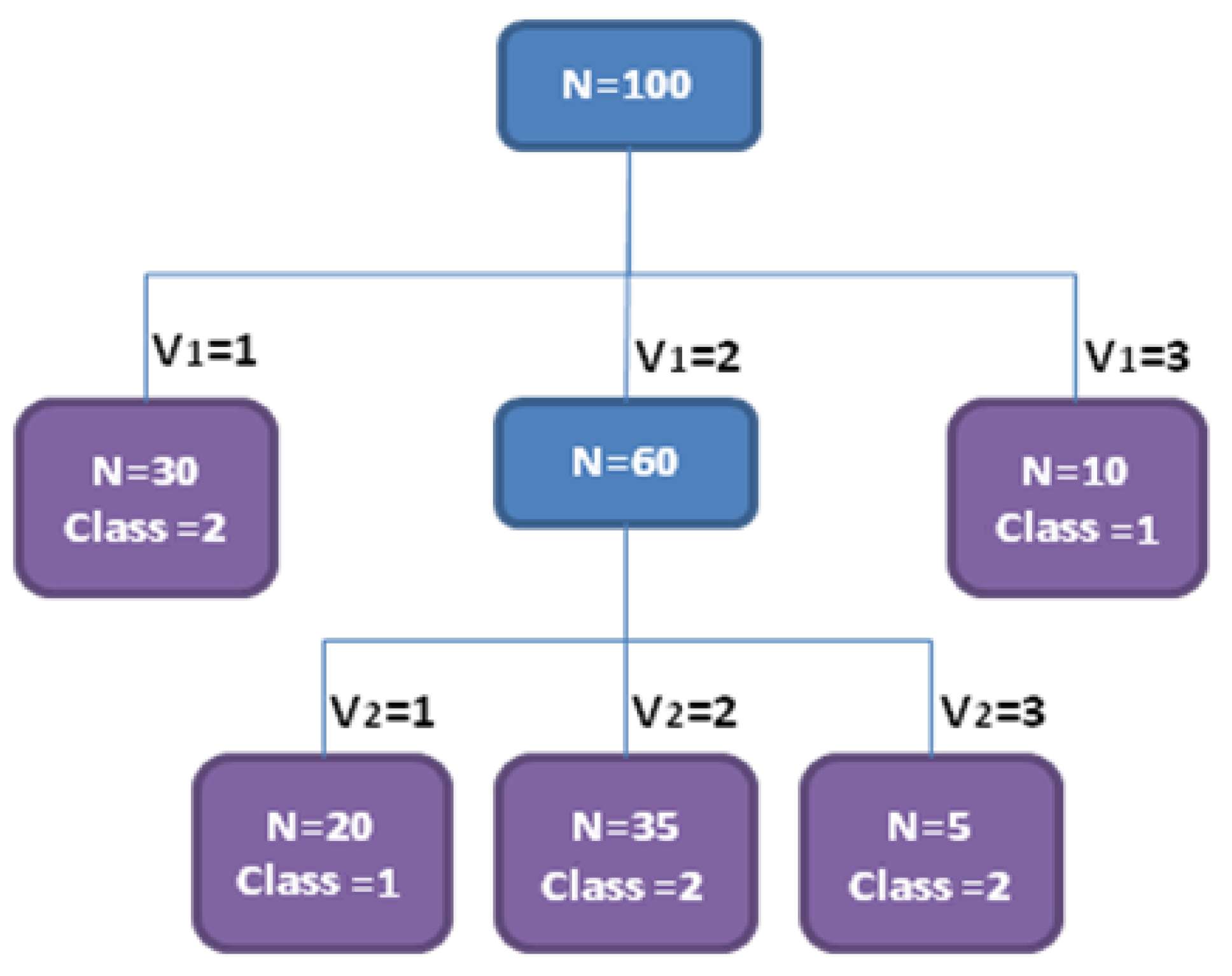
Class 1|Class 2		V2			Total
		1	2	3
V1	1	3|0	1|9	2|0	6|9
	2	6|2	08|12	3|3	17|17
	3	0|1	0|6	0|1	0|8
Total		9|3	09|27	5|4	23|34

In this case, the set of rules is the following:

No.	Premise	Conclusion	Precision
1	V1 = 1	Class = 2	60%
2	V1 = 2, V2 = 1	Class = 1	75%
3	V1 = 2, V2 = 2	Class = 2	60%
4	V1 = 2, V2 = 3	Class = 1	50%
5	V1 = 3	Class = 1	00%

Consider the rule (3):

If V1 = 2 and V2 = 2 then Class = 2,

two rules can be obtained alternatively by pruning it:

• (3.1) If V1 = 2 then Class = 2, or
• (3.2) If V2 = 2 then Class = 2;

where rules (3.1) and (3.2) have respectively precisions of 50% and 75%. In this case, rule (3.2) is an improvement concerning (3). Note that such an improvement can not be achieved applying a tree-based pruning strategy (for the tree of Figure 2), since variable V2 is not used for segmenting in the first level.

6.2. Strengths of Rule Based Post-Pruning Methods

The convenience of converting the decision tree in a set of rules can be summarized in the following points:

• The post-pruning of rules ensures greater flexibility and widest exploration of the hypothesis space. Since each path in the tree (from the root to a leaf (terminal node)) becomes into a different rule, the antecedents (precondition) can be removed iteratively in any order, being possible to consider any combination of antecedents of the rule. On the other hand, whether the growing of the tree is truncated or the post-pruning is performed over the tree, the search space is more limited, since, in the corresponding set of classification rules, any pair of rules is constrained to have a common trunk of antecedents.
• The conversion to rules avoids the removal priority induced by the level of the nodes.
• Generally, the generated models are more readable. For many people rules are generally easier to understand than tree models. Furthermore, the set of rules is simplified iteratively due to the the removal of either antecedents or complete rules.

6.3. Measuring Goodness of Fit for a Sorted List of Rules

We consider the F-measure see [39] to measure the goodness of fit for a rules based classification model. It takes into account both the precision and the recall capability (the capacity to classify correctly the items of a class).

Considering the following table where the membership prediction for a class A is crossed with its real membership for a general case:

		Prediction
		YES	NO
Real	YES	True Positives (TP)	False Negatives (FN)
	NO	False Positives (FP)	True Negatives (TN)

Then the precision is defined as the ratio of the number of items of A correctly classified by the model, over the total number of items labeled as members of A according to the model prediction:

$$P_A=\frac{\mathrm{TP}}{\mathrm{TP}+\mathrm{FP}}.$$

While the recall is defined as the ratio of the number of items from class A correctly classified by the model, over the total number of items that truly belong to A:

$$R_A=\frac{\mathrm{TP}}{\mathrm{TP}+\mathrm{FN}}$$

Finally the F-Measure is defined as

$${\displaystyle F_{\beta }=\frac{(1+{\beta }^2)\overline{P}\overline{R}}{{\beta }^2\overline{P}+\overline{R}},}$$

where $\overline{P}$ and $\overline{R}$ are respectively the average precision and recall over all the classes: $\overline{P}=\frac{1}{C}{\sum }_{i=1}^C{P}_{A_i}$, $\overline{R}=\frac{1}{C}{\sum }_{i=1}^C{R}_{A_i}$, and C is the total number of classes.

The coefficient $\beta$ controls the trade-off between precision and recall. In case of $F_1$, the precision is assigned the same weight as the recall and coincides with the mean of $\overline{P}$ and $\overline{R}$. If $\beta >1$ the recall has greater weight, and if $0<\beta <1$ the precision has greater weight.

Note that $F_{\beta }\in [0,1]$ since $\overline{P},\overline{R}\in [0,1]$ and the following inequalities are equivalent:

$$\begin{array}{ccc}\hfill F_{\beta }& \le & 1\hfill \\ \hfill (1+{\beta }^2)\overline{P}\overline{R}& \le & {\beta }^2\overline{P}+\overline{R}\hfill \\ \hfill (1+{\beta }^2)\overline{P}\overline{R}-{\beta }^2\overline{P}-\overline{R}& \le & 0\hfill \\ \hfill \overline{P}\overline{R}+{\beta }^2\overline{P}\overline{R}-{\beta }^2\overline{P}-\overline{R}& \le & 0\hfill \\ \hfill \overline{R}(\overline{P}-1)+{\beta }^2\overline{P}(\overline{R}-1)& \le & 0.\hfill \end{array}$$

The last one is verified easily since $(\overline{P}-1)\le 0$ and $(\overline{R}-1)\le 0$, therefore, both summands are non-positive.

Values of F-measure near 0 mean that the classification proposed by the model is very poor, while values near 1 indicate that the classification is almost perfect. This measure is frequently used in the area of Information Retrieval to assess the performance of the search and classification of documents. It is also used in Machine Learning to evaluate classification models.

6.4. Simulated Annealing as a Search Strategy

Generally, the precision and fitness of the obtained rules of the based classification model are closely related to the strategy to broaden the search spectrum. A simple idea is following a greedy criterion, by removing a node to produce improvement in precision (but only if the elimination of one generates an improvement, otherwise the rule remains intact). This heuristic is comprehensible, simple and quite efficient regarding the computational cost, but it faces the typical disadvantages of hill-climbing such as local optimization since only a limited part of the search space is explored.

The use of meta-heuristics is an alternative with better results in the exploration of generic and wide search spaces. In particular, for the case of the TAID tree rules, it is significant to implement a Simulated Annealing strategy.

Simulated Annealing (SA) see [40,41] is frequently used in combinatorial optimization problems with discrete search spaces (as is the space of rule antecedents combinations). This method is an adaptation of the Metropolis–Hastings algorithm, a Monte Carlo method for generating samples of states in a thermodynamical system. Zarandia et al. [42] have used it for parameters optimization in fuzzy rules models.

For some problems, SA can be more efficient than exhaustive enumeration since the goal is to find a reasonable solution on a fixed time and not necessarily the best available solution.

The name and inspiration of the SA method arise from the annealing in metallurgy, a technique that involves the heating and controlled cooling of a material to increase the size of its crystals and reduce its defects. The heat causes the atoms to move away from their initial positions (a local minimum of internal energy) and reach states of greater energy, while the slow cooling allows finding configurations with less energy than the initial one.

By analogy with the physical process, each step of the SA algorithm tries to replace the current solution by a random one (generally near the current one) chosen according to certain candidate probability distribution. The new solution is accepted with a probability that depends on the variation of the objective function (function to be optimized) between the current and the new solution, and a global parameter T, called temperature, which decreases gradually in time during the process.

With E being the current energy of the system and $E^{\prime }$ the corresponding to a new state, it is usually proposed that if $E>E^{\prime }$ the new state is accepted with probability $p_a=1$, otherwise, it is accepted with a probability that decreases with the increase on energy and the decrease on temperature. Hence, we consider the following expression:

$$p_a=e^{\frac{(E-E’)}{T}}.$$

6.5. Simulated Annealing for TAID Rules

With the objective to implement the SA algorithm for our TAID rules-based classification model, we propose its configuration according to these points:

• A candidate solution consists of a sorted list of rules (that represent our model).
• The initial solution is obtained from the TAID tree (with rules sorted decreasingly according to their precision).
• The neighbors (candidate successors) of a solution are generated by considering the elimination of one antecedent in each rule and any permutation of the rules.
• The F-measure (see Section 6.3) is considered as a function to be maximized, i.e., the energy of the system is the opposite of the F-measure. The F-measure of the model is computed according to the validation set.

7. TAID-LCA Implementation

The TAID-LCA algorithm has been implemented in R language R [43] that uses some library such as poLCA [44] and rpart [45]. R is a free software project that provides a framework for computational statistics and graphics generation over a programming language of the same name. It is widely used by researchers from diverse disciplines due to the computation facilities it offers (its availability for a wide range of Windows, MacOS, and UNIX platforms) as well as the large number of packages with specific purposes available in its repositories.

In particular, for the LCA, the package poLCA [44], was used, it allows fitting a latent class model from a dataset with nominal variables (previously coded into a numerical scale). For the output of the LCA, the format of Comma Separated Values (CSV) was considered to represent datasets based on a text file format. All this with the purpose of integrating techniques that allow robust segmentation.

The segmentation algorithm was implemented directly, widely exploiting the resources for the numerical and algebraical treatment of matrices such as the singular value decomposition. The XML file format was chosen as the output format for representing the ternary tree model. XML is a standard widely used for data exchange among different applications (either web or desktop and from diverse operating systems). Furthermore, since it is based on text files, it has a friendly approach to be interpreted by a human being.

To provide a friendly interface to a potential user, a desktop application has also been implemented (currently only available for Microsoft Windows operating system) for the C# programming language and .Net platform. This application has the following main functionalities:

• Browse and load the dataset file (input) to be analyzed. Different column separator characters can be specified. New columns can be added, and the values for the variables can be set or modified.
• Specify the explanatory and manifest variables. Optionally, a frequencies column for the dataset records can be specified.
• Specify the LCA parameters.

  –

  The maximum number of iterations of the Expectation-Maximization (EM) algorithm launched by the LCA.

  –

  The number of repetitions (initializations) of the EM algorithm.

  –

  The range for the number of classes (different models) to be considered.

• Set the parameters for the stop conditions of the segmentation algorithm.

  –

  The minimum ratio of items that a node should contain with respect to the total sample size can be partitioned.

  –

  The minimum p-value associated to the CATANOVA index in the significance test (a p-value smaller than this threshold suggests to continue partitioning).

  –

  The impurity index to be used: Gini or Cross-Entropy.

  –

  The impurity tolerance (an impurity greater than this threshold suggests that partitioning should continue).

• Show the fit parameters for the LCA models (marginal and posterior probabilities), as well as some goodness of fit indicators.
• Show a graphical representation of the tree generated by the algorithm, it can be saved as image in different file formats: PNG, JPG, BMP, TIFF or PDF.
• Know details about the segmentation in each node:

  –

  The variable and collapsed categories used in the segmentation that generated the node.

  –

  The number of items contained in the node.

  –

  The proportions corresponding to each class.

  –

  The $\tau$ index value for the variable of greatest explanatory capability.

  –

  The CATANOVA index p-value.

  –

  The impurity measure value.

• Show a graphical representation in the plane of the NSCA between the response variable and the best explanatory one in non-terminal nodes.
• Generate a set of rules from the tree model.
• Perform the rule based post-pruning in a SA algorithm and compare the models before and after the pruning.

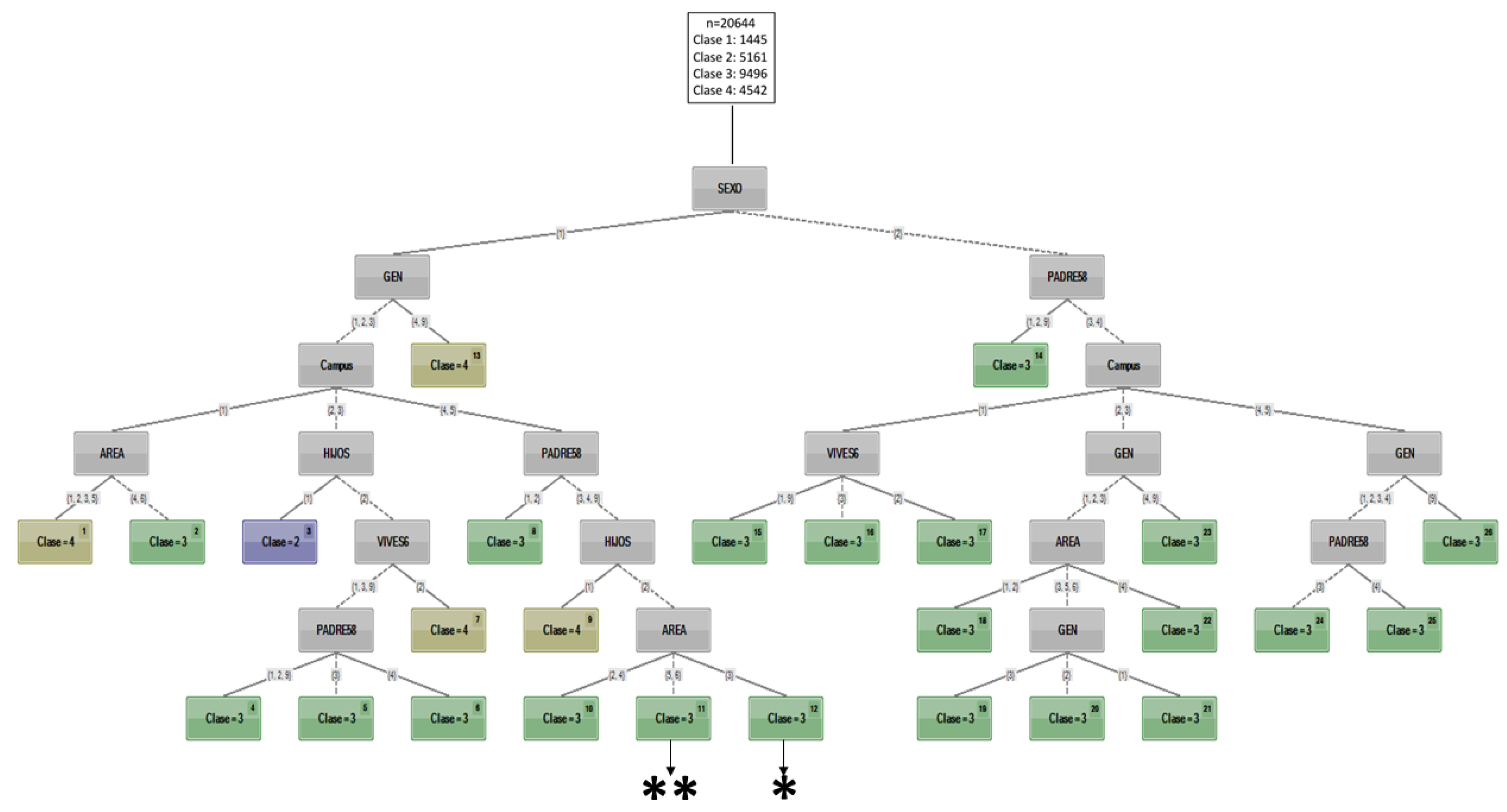
7.1. TAID-LCA Application

Characterization of legal and illegal drugs users segmentation, using TAID-LCA analysis.

The data correspond to the PERCIBETE survey; it aims to know the prevalence of legal and illegal drugs consumption, the issues, and the risk perception of the students. The instrument that was used for the diagnosis of the students’ drugs consumption was called “Questionnaire about the drug’s consumption in students” with 73 items, 20,644 Universidad Veracruzana’s male students participated.

The steps of the algorithm are:

• Find a latent variable of the manifested variables employing the LCA and consider this one as the target variable.
• The root node is made up of the complete sample. Repeat while there is at least one non-terminal node (recursive partition loop).
• Choose a non-terminal node and perform the following steps within it
  • Choose the best explanatory variable concerning the target variable, according to the $\tau$ index.
  • Perform the Non-Symmetrical Correspondence Analysis (NSCA) for the best explanatory variable and the target one.
  • Segment according to the weak, left strong, and right strong categories,
  • Test whether the new nodes are terminal or not, regarding the stop criteria.

7.2. Variables Used

Predictives: Gender (1 man, 2 woman); Zone (1 capital, 2 port, 3 mountains, 4 north, 5 south); Department (1 arts, 2 biology, 3 health, 4, economy, 5 humanities, 6 sciences); System (1 face to face, 2 remote).

Manifest: (1) During the past 12 months, have you smoked tobacco?; (2) During the past 30 days, have you smoked tobacco?; (3) During the past 12 months, have you taken amphetamines or any other stimulants without a doctor’s prescription?; (4) During the past 12 months, have you taken any sedatives without a doctor’s prescription?; (5) During the past 12 months, have you consumed Cannabis?; (6) During the past 12 months, have you consumed cocaine? with the following options as answers: 1.Yes, 2.No, 3.Not for this case, and 4.Not specified. Additionally, (7) Use and abuse of alcohol: 1. Risk consumption, 2. Abusive consumption, 3. Moderate consumption 4 Not specified; and (8) How often do you get drunk? 1. Never in the last year, 2. At least once in the last year, 3. Once in the last month, 4. Once or more in the last month, 5. Not specified.

The elbow criterion suggested choosing the 4 classes model:

• Class 1: Smokers-alcohol abusers and have consumed Cannabis.
• Class 2: Moderate-alcohol drinkers and who get drunk.
• Class 3: Moderate-alcohol drinkers who get drunk.
• Class 4: Smokers and moderate-alcohol consumers

The output of the TAID-LCA is a ternary tree show in Figure 3, yielded from the recursive partition by the values of the explanatory variables, where the latent variable is the target one (it summarizes the manifest variables).

✱

Male students in port and mountain regions, from the economy department, are mostly classified in latent class 3.

✱✱

Male students in capital regions, from the arts department, are mostly classified in latent class 3.

8. Conclusions

We have demonstrated that the predictivity factorial decomposition provides parsimonious models for asymmetric two-dimension contingency tables, which allow establishing criteria for the collapsibility of categories of predictor variables and detect categories with a weak prediction for subsequent segmentation.

We have proposed a ternary tree segmentation algorithm that enables working with the multivariable explanatory variable and choosing terminal segments with a strong prediction for the latent explanatory latent which collects the multivariant information of the response variable, only for the use of categorized variables.

The provided segments by the algorithm have not only a high predictive characteristic for the target response but also the manifest.

The development and programming of TAID-LCA in the real data application have shown the practical interest of our theoretical contributions.

References

- Kass, G. An Exploratory Technique for Investigating Large Quantities of Categorical Data. J. Appl. Stat. 1980, 29, 127–199. [Google Scholar] [CrossRef]
- Morgan, J.; Sonquist, J. Problems in the Analysis of Survey Data and A Proposal. J. Am. Satistical Assoc. 1963, 67, 768–772. [Google Scholar] [CrossRef]
- Antipov, E.; Pokryshevskaya, E. Applying CHAID for logistic regression diagnostics and classification accuracy improvement. J. Target. Meas. Anal. Mark. 2010, 18, 109–117. [Google Scholar] [CrossRef]
- Antipov, E.; Pokryshevskaya, E. Profiling satisfied and dissatisfied hotel visitors using publicly available data from a booking platform. Int. J. Hosp. Manag. 2017, 67, 1–10. [Google Scholar]
- StatSoft. STATISTICA 10.0; StatSoft, Inc.: Tulsa, OK, USA, 2010. [Google Scholar]
- IBM Corp. IBM SPSS Statistics for Windows, Version 27.0; IBM Corporation: Endicott, NY, USA, 2020. [Google Scholar]
- Hothorn, T.; Zeileis, A. partykit: A modular toolkit for recursive partytioning in R. J. Mach. Learn. Res. 2015, 16, 3905–3909. [Google Scholar]
- Breiman, L.; Friedman, J.; Olsen, R.; Stone, C. Classification and Regression Trees; Chapman and Hall: London, UK, 1984. [Google Scholar]
- Galindo-Villardón, P.; Vicente-Villardón, J.L.; Díaz, A.D.; Vicente-Galindo, P.; Patino-Alonso, M.C. An alternative to CHAID segmentation algorithm based on entropy. Rev. Mat. Teor. Y Apl. CIMPA—UCR 2010, 17, 185–204. [Google Scholar]
- Avila, C.A. Una Alternativa al Análisis de Segmentación Basada en el Análisis de Hipótesis de Independencia Condicionada. Ph.D. Thesis, Universidad de Salamanca, Salamanca, Spain, 1996. [Google Scholar]
- Dorado-Díaz, A. Métodos de Búsqueda de Variables Relevantes en Análisis de Segmentación: Aportaciones desde una Perspectiva Multivariante. Ph.D. Thesis, Universidad de Salamanca, Salamanca, Spain, 1998. [Google Scholar]
- Castro, C.; Galindo, P. Colapsabilidad de Tablas de Contingencia Multivariantes; Editorial Académica Española: Alemania, Germany, 2011. [Google Scholar]
- Siciliano, R.; Mola, F. Ternary Classification Trees: A Factorial Approach. In Visualization of Categorical Data; Academic Press: Cambridge, MA, USA, 1997; Chapter 22; pp. 311–323. [Google Scholar]
- Gunduz, M.; Lutfi, H. Go/No-Go Decision Model for Owners Using Exhaustive CHAID and QUEST Decision Tree Algorithms. Sustainability 2021, 13, 815. [Google Scholar] [CrossRef]
- Djordjevic, D.; Cockalo, D.; Bogetic, S.; Bakator, M. Predicting Entrepreneurial Intentions among the Youth in Serbia with a Classification Decision Tree Model with the QUEST Algorithm. Mathematics 2021, 9, 1487. [Google Scholar] [CrossRef]
- Lauro, N.; D’ambra, L. L’analyse non symétrique des correspondances. Data Anal. Inform. 1984, 3, 433–446. [Google Scholar]
- Lazarsfeld, P.F.; Henry, N.W. Latent Structure Analysis; Houghton Mifflin: Boston, MA, USA, 1968. [Google Scholar]
- Goodman, L.A. Exploratory latent structure analysis using both identifiable and unidentifiable models. Biometrika 1974, 61, 215–231. [Google Scholar] [CrossRef]
- Lindsay, B.; Clogg, C.C.; Greco, J. Semiparametric estimation in the Rash model and related exponential response models, including a simple latent class model for item analysis. J. Am. Satistical Assoc. 1991, 86, 96–107. [Google Scholar] [CrossRef]
- Uebersax, J.S. Statistical modeling of expert ratings on medical treatment appropriateness. J. Am. Satistical Assoc. 1993, 88, 421–427. [Google Scholar] [CrossRef]
- Magidson, J.; Vermunt, J. Latent class factor and cluster models, bi-plots and related graphical displays. Sociol. Methodol. 2001, 31, 223–264. [Google Scholar] [CrossRef]
- Reyna, C.; Brussino, S. Revisión de los fundamentos del análisis de clases latentes y ejemplo de aplicación en el área de las adicciones. Trastor. Adict. 2011, 13, 11–19. [Google Scholar] [CrossRef]
- Araya Alpízar, C. Modelos de clases latentes en tablas poco ocupadas: Una contribución basada en bootstrap. Ph.D. Thesis, Universidad de Salamanca, Salamanca, Spain, 2010. [Google Scholar]
- Lanza, S.T.; Rhoades, B.L. Latent class analysis: An alternative perspective on subgroup analysis in prevention and treatment. Prev. Sci. 2013, 14, 157–168. [Google Scholar] [CrossRef] [Green Version]
- Oberski, D.; van Kollenburg, G.; Vermunt, J. A Monte Carlo evaluation of three methods to detect local dependence in binary data latent class models. Adv. Data Anal. Classif. 2013, 7, 267–279. [Google Scholar] [CrossRef]
- McLanchlan, L.; Basford, M. Mixture Models: Inference and Appliccation to Clustering; Marcel Dekker: New York, NY, USA, 1988. [Google Scholar]
- Fop, S.K.M.; Murphy, T. Variable Selection for Latent Class Analysis with Application to Low Back Pain Diagnosis. Ann. Appl. Stat. 2017, 11, 2085–2115. [Google Scholar] [CrossRef] [Green Version]
- Gonçalves, T.; Lourenço-Gomes, L.; Pinto, L. Modelling consumer preferences heterogeneity in emerging wine markets: A latent class analysis. Appl. Econ. 2020, 52, 6136–6144. [Google Scholar] [CrossRef]
- Goodman, L.A. Simple Models for The Analysis of Association in Cross-Classification Having Order Categories. J. Am. Satistical Assoc. 1979, 74, 537–552. [Google Scholar] [CrossRef]
- Goodman, L.A. The Analysis of Cross-classified Data Having Ordered and/or Unordered Categories: Association Models, Correlation Models and Asymmetry Models for Contingency Tables with or without Missing Entries. Ann. Stat. 1985, 13, 10–69. [Google Scholar] [CrossRef]
- Wermuth, N.; Cox, D.R. On the Application of Conditional Independence to Ordinal Data. Int. Stat. Rev. 1998, 66, 181–199. [Google Scholar] [CrossRef]
- Gilula, Z.; Krierger, A.M. Collapsed Two-Way Contingency Tables and the Chi-square Reduction Principle. J. Am. Satistical Assoc. 1989, 51, 424–433. [Google Scholar] [CrossRef]
- Lauro, N.C.; D’Ambra, L. L’analyse non symétrique des correspondances. In Data Analysis and Informatics; Data Analysis and Informatics III; Elsevier: Amsterdam, The Netherlands, 1984; pp. 433–446. [Google Scholar]
- Goodman, L.; Kruskal, W. Measures of association for cross classifications. J. Am. Satistical Assoc. 1954, 49, 732–764. [Google Scholar]
- Light, R.; Margolin, B. An analysis of variance for categorical data. J. Am. Satistical Assoc. 1971, 66, 534–544. [Google Scholar] [CrossRef]
- Olmuş, H.; Erbaş, S. Catanova method for determining of zero partial association structures in multidimensional contigency tables. Gazi Univ. J. Sci. 2014, 27, 953–963. [Google Scholar]
- Tan, P.N.; Steinbach, M.; Kumar, V. Introduction to data mining; Pearson Education India: Delhi, India, 2016. [Google Scholar]
- Mitchell, T. Machine Learning; McGraw Hill: New York, NY, USA, 1997; pp. 66–72. [Google Scholar]
- Van Rijsbergen, C.J. Information Retrieval; Butterworth-Heinemann: Oxford, UK, 1979; p. 224. [Google Scholar]
- Kirkpatrick, S.; Gelatt, C.J.; Vecchi, M.P. Optimization by Simulated Annealing. Science 1983, 220, 671–680. [Google Scholar] [CrossRef] [PubMed]
- Aarts, E.; van Laarhoven, P. Simulated annealing: An introduction. Stat. Neerl. 1989, 43, 31–52. [Google Scholar] [CrossRef]
- Zarandia, M.F.; Zarinbala, M.; Ghanbaria, N.; Turksen, I. A new fuzzy functions model tuned by hybridizing imperialist competitive algorithm and simulatedannealing. Application: Stock price prediction. Inf. Sci. 2012, 217, 213–228. [Google Scholar]
- R Development Core Team. R: A Language and Environment for Statistical Computing; R Foundation for Statistical Computing: Vienna, Austria, 2020; ISBN 3-900051-07-0. [Google Scholar]
- Linzer, D.A.; Lewis, J.B. poLCA: An R Package for Polytomous Variable Latent Class Analysis. J. Stat. Softw. 2011, 42, 1–29. [Google Scholar] [CrossRef] [Green Version]
- Therneau, T.; Atkinson, B. rpart: Recursive Partitioning and Regression Trees; R Package Version 4.1-15. Available online: https://cran.r-project.org/web/packages/rpart/rpart.pdf (accessed on 1 December 2021).
Publisher’s Note: MDPI stays neutral with regard to jurisdictional claims in published maps and institutional affiliations. |
© 2022 by the authors. Licensee MDPI, Basel, Switzerland. This article is an open access article distributed under the terms and conditions of the Creative Commons Attribution (CC BY) license (https://creativecommons.org/licenses/by/4.0/).
Share and Cite
Castro-López, C.; Vicente-Galindo, P.; Galindo-Villardón, P.; Borrego-Hernández, O. TAID-LCA: Segmentation Algorithm Based on Ternary Trees. Mathematics 2022, 10, 560. https://doi.org/10.3390/math10040560
Castro-López C, Vicente-Galindo P, Galindo-Villardón P, Borrego-Hernández O. TAID-LCA: Segmentation Algorithm Based on Ternary Trees. Mathematics. 2022; 10(4):560. https://doi.org/10.3390/math10040560
Chicago/Turabian StyleCastro-López, Claudio, Purificación Vicente-Galindo, Purificación Galindo-Villardón, and Oscar Borrego-Hernández. 2022. "TAID-LCA: Segmentation Algorithm Based on Ternary Trees" Mathematics 10, no. 4: 560. https://doi.org/10.3390/math10040560
APA StyleCastro-López, C., Vicente-Galindo, P., Galindo-Villardón, P., & Borrego-Hernández, O. (2022). TAID-LCA: Segmentation Algorithm Based on Ternary Trees. Mathematics, 10(4), 560. https://doi.org/10.3390/math10040560