Permutation Variation and Alternative Hyper-Sphere Decomposition

Abstract

Current covariance modeling methods work well in longitudinal data analysis. In the analysis of data with no nature order, a common covariance modeling method would be inadequate. In this paper, a study is implemented to investigate the effects of permutations of data on the estimation of covariance matrix $\Sigma$. Based on the Hyper-sphere decomposition method (HPC), this study suggests that the change of data’s permutation breaks the consistency of covariance estimation. An alternative Hyper-sphere decomposition method with permutation invariant is introduced later in this paper. The alternative method’s consistency and asymptotic normality are studied when the observations follow a normal distribution. These results are tested using some example studies. Furthermore, a real data analysis is conducted for illustration purposes.

1. Introduction

The covariance matrix is a simple and popular method to describe the variation and correlation between random variables in multivariate statistics. A valid covariance matrix must be symmetric and semi-positive definite. In some areas, like social sciences, finance, economics and geology, people are more interested in studying the covariance matrices than mean models. Meanwhile, an appropriate working covariance matrix could increase the estimator’s efficiency. Moreover, Pourahmadi (2013) [1] suggests a good estimate of the covariance matrix can lead to an accurate statistical inference and test results. Little and Rubin (2019) [2] show that an accurate estimate of covariance is essential in dealing with missing data problems. A sample covariance is usually used to estimate the population covariance matrix for its convenience. In some special cases, for example, high-dimensional situations where the number of repeated measurements n is less than that of unknown parameters in covariance matrix, using sample covariance matrix would end up with a biased estimator of mean model [3].

Pourahmadi (1999) [4] introduced the modified Cholesky decomposition method (MCD ) into the estimation of covariance matrix by applying regression-based ideas into matrix decomposition methods. However, the interpretation of the relationship between model coefficients and correlation/variance of population Y is indirect. Pan and Pan (2017) [5] proposed the alternative Cholesky decomposition method (ACD) in 2017 that improves the correlation-interpretation problem of MCD by applying Cholesky decomposition on the correlation matrix R,

$$\Sigma =DRD=DT{T}^{\prime }D,$$

where matrix D is a diagonal matrix with standard deviations $\sigma$ of population Y, and T is a lower-triangular matrix with unit row vectors, ${\overrightarrow{T}}_{\left(i\right)}$$i=1,\cdots ,p$, whose Euclidean norm is 1. The same model regression procedure as in MCD cannot be applied in ACD due to the extra unit-norm-restriction on row vectors in matrix T. Rebonato and Jäckel (2011) [6] projected T in ACD into a unit Hyper-sphere coordinate system and proposed the Hyper-sphere decomposition method (HPC), in which elements $t_{ij}$ in T are

$$t_{ij}=\left\{\begin{array}{cc}1\hfill & i=j=1\hfill \\ cos{\varphi }_{ij}\prod _{k=1}^{j-1}sin{\varphi }_{ik}\hfill & j=1,\dots ,p-1,i=2,\cdots ,p\hfill \\ \prod _{k=1}^{j-1}sin{\varphi }_{ik}\hfill & j=p\hfill \end{array}\right.,$$

(1)

where ${\varphi }_{jk}$ are corresponding new angular coordinates of vector ${\overrightarrow{T}}_{\left(i\right)}$ in a unit hyper-sphere coordinate system. As a result we have

$$T=\left(\begin{array}{ccccc}1& 0& 0& \cdots & 0\\ c_{21}& s_{21}& 0& \cdots & 0\\ ⋮& ⋮& ⋮& \ddots & ⋮\\ c_{p,1}& c_{p,2}{s}_{p,1}& c_{p,3}{s}_{p,2}{s}_{p,1}& \cdots & {\prod }_{k=1}^p{s}_{p,k}\end{array}\right),$$

where $c_{ij}\mathrm{and}{s}_{ij}$ refer to $cos\left({\varphi }_{ij}\right)\mathrm{and}sin\left({\varphi }_{ij}\right)$. Comparing to ACD there is an additional matrix $\Phi$, which is also a lower triangular with diagonal elements 0 and with the lower off-diagonal being angles ${\varphi }_{ij}\in [0,\pi )$,

$$\Phi =\left(\begin{array}{cccccc}0& 0& 0& \cdots & 0& 0\\ {\varphi }_{21}& 0& 0& \cdots & 0& 0\\ {\varphi }_{31}& {\varphi }_{32}& 0& \cdots & 0& 0\\ ⋮& ⋮& ⋮& \ddots & ⋮& ⋮\\ {\varphi }_{p1}& {\varphi }_{p2}& {\varphi }_{p3}& \cdots & {\varphi }_{p,p-1}& 0\end{array}\right).$$

This method can guarantee the unit-row vectors in T for any given estimator matrix $\Phi$; meanwhile, this decomposition has a geometry meaning for $\Phi$  [7]. In that sense, the regular model regression procedure can be applied in HPC just as in Pourahmadi (2000) [8]. To ensure ${\varphi }_{jk}\in [0,\pi )$ we can do a further triangular transpose on the liner model:

$$\begin{array}{cccc}tan({\varphi }_{jk}-{\displaystyle \frac{\pi }{2}})={\omega }_{jk}^{\prime }\gamma \hfill & \varphi \in [0,\pi ),& \mathrm{and}& \hfill log{\sigma }_j^2=h_j^{\prime }\lambda ,\end{array}$$

(2)

where ${\omega }_{jk}$ and $h_j$ are design matrices and vectors for angles ${\varphi }_{jk}$ and variances ${\sigma }_j^2$, respectively. Meanwhile, $\gamma$ and $\lambda$ in Equation (2) are unknown correlation and variance components.

The current popular methods like HPC work well in longitudinal data analysis in which there is a natural order of the sample data. While in analyses like geometric and causal data there is no natural permutation of data, these methods generate estimates that depend on the permutation of sample data. The purpose of this article is to illustrate the permutation variance of covariance estimator of HPC. After that, we redefine the translation between T and $\Phi$, then propose an alternative Hyper-sphere decomposition (AHPC) method that inherits most of the advantages of HPC while improving the permutation variance. Meanwhile, the AHPC has a more straightforward geometrical interpretation.

2. Interpretations of Hyper-Sphere Decomposition Method

Rapisarda, Brigo and Mercurio (2007) [7] explained HPC from the aspect of Jacobi rotation. In a p-dimensional right-hand system, axis $e_1,e_2,\cdots ,e_p$ are selected as follows:

1.

Set the direction of ${\overrightarrow{T}}_{\left(1\right)}$ as the first axis $e_1$.

2.

In the plane containing vectors ${\overrightarrow{T}}_{\left(1\right)}$ and ${\overrightarrow{T}}_{\left(2\right)}$, make the $e_2$ vertical to $e_1$ in a right-hand system.

3.

$e_3$ is perpendicular to the previous axis, $e_1$ and $e_2$, and on the same side of their cross product $e_1\times e_2$.

4.

After the signed j axis, the next axis $e_{j+1}$ is defined as vertical to all previous axes and on the same direction of $e_1\times e_2\cdots \times e_j$, while $j+1\le p$.

Cross product $e_j\times e_k=\left|\right|e_j\left|\right|·\left|\right|e_k\left|\right|sin\theta ·\overrightarrow{n}$ determines a direction $\overrightarrow{n}$ perpendicular to the plane containing $e_j$ and $e_k$ given by the right-hand rule.

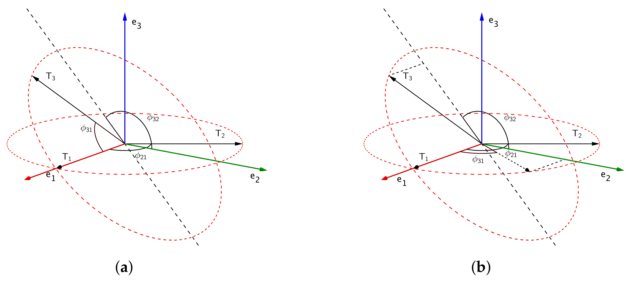
With all axes having been set up, the row vectors ${\overrightarrow{T}}_{\left(j\right)}={\left(t_{j1},\cdots ,t_{jj},0,\cdots ,0\right)}^{\prime }$ shows us the coordinate of ${\overrightarrow{T}}_{\left(j\right)}$ in this Cartesian system. According to  [7], the relation between angles ${\varphi }_{ij}$ and coordinates of ${\overrightarrow{T}}_{\left(k\right)}$s is (Figure 1a):

1.

We begin with ${\overrightarrow{T}}_{\left(1\right)}$. Next we turn ${\overrightarrow{T}}_{\left(1\right)}$ counter-clockwise in hyper-plane $P{L}_{12}$ with angle ${\varphi }_{2,1}$. Then we have ${\overrightarrow{T}}_{\left(2\right)}=G(1,2;{\varphi }_{2,1}){\overrightarrow{T}}_{\left(1\right)}$. The hyper-plane $P{L}_{12}$ is built with $e_1$ and $e_2$.

2.

Turn ${\overrightarrow{T}}_{\left(1\right)}$ in $P{L}_{12}$ with angle ${\varphi }_{3,1}$; then do another rotation in $P{L}_{23}$ with angle ${\varphi }_{3,2}$. We then have ${\overrightarrow{T}}_{\left(3\right)}=G(2,3;{\varphi }_{3,2})G(1,2;{\varphi }_{3,1}){\overrightarrow{T}}_{\left(1\right)}$.

3.

${\overrightarrow{T}}_{\left(k\right)}$ is built up with $k-1$ times turn as: ${\overrightarrow{T}}_{\left(k\right)}=G(k-1,k;{\varphi }_{k,k-1})\cdots G(1,2;{\varphi }_{k,1}){\overrightarrow{T}}_{\left(1\right)}$.

In a p-dimensional space, $G(j,k;\theta )$ is a Jacobi rotation matrix in hyper-plane $P{L}_{j,k}$ with counter-clockwise angle $\theta$. Besides the geometric explanation from  [7], we also propose a new interpretation of the correlation between matrices T and $\Phi$ in the HPC method, regarding angles between two hyper-planes in a row space of T (Figure 1b):

1.

Lower off-diagonal entries in the first column of $\Phi$, ${\varphi }_{i1}$s, are angles between the first and ith row vectors in T.

2.

The lower off-diagonal entries in second column of $\Phi$ contains angles, ${\varphi }_{i2}$s, between plane $H{P}_{12}$, which is defined by the first and second row vectors in T, and $H{P}_{1i}$$i>2$, which is defined by the first and ith row vectors in T.

3.

After that, elements ${\varphi }_{jk}$ in kth column of matrix $\Phi$, $j>k\ge 3$, are angles between two hyper-planes $H{P}_{12\cdots (k-1)k}$ and $H{P}_{12\cdots (k-1)j}$.

The $H{P}_{12\cdots k}$’s are built with the first, second and until the kth row vectors. The angle between hyper-planes is well known in the mathematics literature, see, e.g., [Chep. 3] of Murty [9]. The angle ${\varphi }_{jk}$’s between two hyper-planes, $H{P}_{12\cdots (k-1)k}$ and $H{P}_{12\cdots (k-1)j}$ can be calculated recursively via

$${\theta }_{jk}=\left\{\begin{array}{cc}arcos\left(t_{jk}\right)\hfill & j\ge 2,k=1\hfill \\ arcos\left({\displaystyle \frac{t_{jk}}{t_{j(k-1)}tan\left({\theta }_{j(k-1)}\right)}}\right)\hfill & j>2,k\ge 2\hfill \end{array}\right.,$$

(3)

According to [7], when ${\theta }_{jk}$’s and ${\varphi }_{jk}$’s are in $[0,\pi ]$, the translation in Equation (3) is unique, ${\theta }_{jk}={\varphi }_{jk}$.

3. Order-Dependence of Hyper-Sphere Decomposition Method

Based on both explanations of the HPC method above, we show that the HPC is order-dependent from two aspects in this section.

Setting R as a correlation matrix between random sample $Y={(Y_1,\cdots ,Y_p)}^{\prime }$, and after a standard Cholesky decomposition $R=T{T}^{\prime }$, where $T={\left({\overrightarrow{T}}_{\left(1\right)},\cdots ,{\overrightarrow{T}}_{\left(p\right)}\right)}^{\prime }$, based on the definition of HPC decomposition, the correlation ${\rho }_{jk}$ in R is actually the $cosine$ value of an angle between two unit vectors ${\overrightarrow{T}}_{\left(j\right)}$ and ${\overrightarrow{T}}_{\left(k\right)}$, ${\rho }_{jk}={\overrightarrow{T}}_{\left(j\right)}^{\prime }{\overrightarrow{T}}_{\left(k\right)}=cos<{\overrightarrow{T}}_{\left(j\right)},{\overrightarrow{T}}_{\left(k\right)}>$. So eventually we say that these unit vectors ${\overrightarrow{T}}_{\left(j\right)}$ in lower-triangular matrix T represent the whole correlation information of corresponding random sample $Y_j$. In that sense, the order of row vectors in T has almost the same representation of the order of $Y_j$ in correlation matrix R. For example, when $p=6$, under the order $Y_1,Y_2,Y_3,Y_4,Y_5,Y_6$, we have R and the lower triangular T matrix in (4) where, for example, $t_{42}$ is the coordinate on axis $e_2$ for vector ${\overrightarrow{T}}_{\left(4\right)}$, which corresponds to $Y_4$. Then we will have a $\Phi$ matrix as the left one in (5) where in the matrix $\Phi$, from left to right, ${\varphi }_{jk}$ is the kth Jacobi rotation angle in hyper-plane $P{L}_{k,k+1}$, which is built with $e_k$ and $e_{k+1}$. For example, ${\varphi }_{42}$ is the second Jacobi rotation angle in $P{L}_{23}$.

(4)

From the aspect of angles between two hyper-planes, we have the table for matrix $\Phi$ as in the right one in (5) where j stands for row number. In this table, for example, ${\varphi }_{53}$ is the angle between $H{P}_{1,2,3}$ and $H{P}_{1,2,5}$. Hyper-plane $H{P}_{1,2,5}$ is built with the first, second and fifth row vectors in T.

(5)

Eventually we have the same equation between $\rho$ and $\varphi$ as in  [10]:

$${\rho }_{jk}=c_{jk}\prod _{l=1}^{k-1}{s}_{jl}{s}_{kl}+\sum _{l=1}^{k-1}\left[c_{jl}{c}_{kl}\prod _{t=1}^{l-1}{s}_{jt}{s}_{kt}\right],$$

(6)

where $s_{jk}$ and $c_{jk}$ stand for $sin\left({\varphi }_{jk}\right)$ and $cos\left({\varphi }_{jk}\right)$, respectively.

If we change the order of $Y_j$s in correlation matrix R, simultaneously we change the corresponding row vectors, ${\overrightarrow{T}}_{\left(j\right)}$s, in lower-triangular matrix T. While the elements in new matrix $T^{*}$ may change after changing order, the relationship between ${\overrightarrow{T}}_{\left(j\right)}$ and $Y_j$ remains the same. As illustrated before, elements in matrix T are coordinates. When the order of $Y_j$s is different, we set up a new set of axes. That leads us to have a new set of coordinates for ${\overrightarrow{T}}_{\left(j\right)}$s. If we change the order into $Y_1,Y_2,Y_5,Y_4,Y_3,Y_6$, then the new correlation matrix $R^{*}$ can be obtained by swapping elements in R and doing the Cholesky decomposition on $R^{*}$ we get $T^{*}$ as in (7).

(7)

Since we changed the order from position $Y_3$, simultaneously a new set of axes $e_3^{*}$, $e_4^{*}$, $e_5^{*}$ and $e_6^{*}$ are selected. As a result we will have new value for the coordinate on $e_3^{*}$, $e_4^{*}$ and $e_5^{*}$, represented as *s. Meanwhile, the corresponding ${\Phi }^{*}$ matrix will be like in (8).

(8)

From the aspect of Jacobi rotation, element ${\varphi }_{jk}$ in $\Phi$ is a rotating angle in plane $P{L}_{k,k+1}$ built by axes $e_k$ and $e_{k+1}$. Because the definition of axis $e_j$s depend on the order of ${\overrightarrow{T}}_{\left(j\right)}$, which is again also the order of $Y_j$, ${\varphi }_{jk}$ still depends on the order of $Y_j$. We can observe that $cos<{\overrightarrow{T}}_{\left(1\right)},{\overrightarrow{T}}_{\left(k\right)}>={\overrightarrow{T}}_{\left(1\right)}^{\prime }{\overrightarrow{T}}_{\left(k\right)}=(1,\cdots ,0){(c_{k1},\cdots .0)}^{\prime }=c_{k1}=f\left({\varphi }_{k1}\right)$, and $cos<{\overrightarrow{T}}_{\left(2\right)},{\overrightarrow{T}}_{\left(k\right)}>={\overrightarrow{T}}_{\left(2\right)}^{\prime }·{\overrightarrow{T}}_{\left(k\right)}=(c_{21},\cdots ,0){(c_{k1},\cdots ,0)}^{\prime }=c_{21}{c}_{k1}+s_{21}{c}_{k2}{s}_{k1}=f({\varphi }_{21},{\varphi }_{k1},{\varphi }_{k2}),$ which shows that ${\rho }_{1k}$ and ${\rho }_{2k}$ only relay on ${\varphi }_{k1}$, ${\varphi }_{k2}$ and ${\varphi }_{21}$. This explains the reason why ${\varphi }_{k1}$ and ${\varphi }_{k2}$ remain the same, respectively. Since the third vector becomes ${\overrightarrow{T}}_{\left(5\right)}$, angles on the column 3 all will have a new value, except ${\varphi }_{53}$, for obvious reasons, the angle between $H{P}_{1,2,3}^{*}$ and $H{P}_{1,2,5}^{*}$ equals that between $H{P}_{1,2,5}$ and $H{P}_{1,2,3}$.

We summarize this dependency in

Table 1. Dependence between entries in $\Phi$ and row vectors in T. For example, 1, 2, 3, p means element ${\varphi }_{p3}$, at row p column 3 in $\Phi$ depends on the first, second, third and pth row vectors in T.

	col1	col2	col3	...	colp-1	colp
row1	0	0	0	...	0	0
row2	1, 2	0	0	...	0	0
row3	1, 3	1, 2, 3	0	...	0	0
⋮	⋮	⋮	⋮	⋮	⋮	⋮
rowp	1, p	1, 2, p	1, 2, 3, p	...	1, 2, 3, ..., p − 1, p	0

. Table 1 indicates how the value of entries in $\Phi$ depend on the order of row vectors in matrix T.

After proving the permutation variation of the values in the $\Phi$ matrix, we consider how this would affect our modeling process. If the HPC method were permutation invariant, the model assumption should always hold no matter how we change the order of data Y. However, a different order gives different values of $\Phi$, proven above. Then, under the model (2), with the same covariates ${\omega }^{*}$ and $h^{*}$ in which the corresponding values have been rearranged according to the new order, HPC would have a different estimator of $\widehat{\gamma }$ and $\widehat{\lambda }$. In some cases, even the whole model assumption would be wrong under the new permutation of sample data.

Due to the definition of translation between matrices T and $\Phi$, according to our study, the data order affects $\Phi$ element-wise. Furthermore, there is no way of transforming a new angle matrix under the new data order back to its previous one only by rearranging elements. In other words, a change of the order will give a different set of values for $\Phi$. The regression model on $\Phi$ elements would have different parameter estimates under varied data order. Furthermore, even the model assumption may vary according to the data order. In that sense, we say the current HPC method is order dependent. As the conclusion, under both interpretations, the HPC method is permutation variate both in terms of the $\Phi$ matrix and models for variance components.

4. Alternative Hyper-Sphere Decomposition Method

We notice that the order dependency of the HPC method is caused by the definition of the translation between two coordinate systems, the Cartesian coordinate system for matrix T and a unique angular coordinate system for $\Phi$. We now propose a new definition of matrix $\Phi$ inspired by spherical parameterization  [11], which would improve the relationship between matrices R and $\Phi$. Then eventually the newly proposed alternative Hyper-sphere decomposition (AHPC) would be permutation invariant.

4.1. The AHPC Model

The AHPC method differs from HPC in a new definition on $\Phi$, the lower triangular matrix with diagonal elements equal to 0. Instead of being angles between hyper-planes in HPC, here we define our elements in $\Phi$ as angles between row vectors ${\overrightarrow{T}}_{\left(j\right)}$s, as illustrated in Figure 2,

$${\varphi }_{jk}=<{\overrightarrow{T}}_{\left(j\right)},{\overrightarrow{T}}_{\left(k\right)}>1<k<j\le p,$$

(9)

where ${\varphi }_{jk}\in [0,\pi )$ to ensure the uniqueness.

For dimension $p\ge 3$, there is a three-dimensional restriction. Any pairs of vectors $T_i$ and $T_j$ must be in a two-dimensional plan, the angle ${\varphi }_{ij}\in [0,\pi )$ between ${\overrightarrow{T}}_{\left(i\right)}$ and ${\overrightarrow{T}}_{\left(j\right)}$, to guarantee the uniqueness. Furthermore, for angles between three vectors, there are only two proper situations. The first one is ${\varphi }_{jk}={\varphi }_{ji}+{\varphi }_{ik}$ when vector ${\overrightarrow{T}}_{\left(i\right)}$, ${\overrightarrow{T}}_{\left(j\right)}$ and ${\overrightarrow{T}}_{\left(k\right)}$ are in the same plane, and ${\overrightarrow{T}}_{\left(i\right)}$ is sitting between ${\overrightarrow{T}}_{\left(j\right)}$ and ${\overrightarrow{T}}_{\left(k\right)}$. The second scenario is ${\varphi }_{jk}<{\varphi }_{ji}+{\varphi }_{ik}$ where three vectors are not in the same plane. Consequently, for any three vectors ${\overrightarrow{T}}_{\left(i\right)}$, ${\overrightarrow{T}}_{\left(j\right)}$ and ${\overrightarrow{T}}_{\left(k\right)}$, angles between each pair of vectors must satisfy that the sum of any two angles be not less than the third one and the difference between any two angles be not greater than the third one,

$${\varphi }_{jk}\le {\varphi }_{ji}+{\varphi }_{ik}\mathrm{and}{\varphi }_{jk}\ge {\varphi }_{ji}-{\varphi }_{ik},k<i<j,$$

(10)

where ${\varphi }_{ji}={\varphi }_{ij}$. Thus for the restriction on angles between vectors in three-dimensional spaces, the model assumption must satisfy the constraint ${\varphi }_{jk}\le {\varphi }_{ij}+{\varphi }_{ik}$. This is not only due to the geometric fact but also is sufficient for positive semi-definiteness of correlation matrix R. When ${\varphi }_{jk}={\varphi }_{ji}+{\varphi }_{ik}$, $T_i$, $T_j$ and $T_k$ must be on the same plane, which suggests that there must exist constants a and b such that $T_i=a{T}_j+b{T}_k$. As a result, in the ith row of correlation matrix R,

$${\rho }_{ih}=T_i^{\prime }{T}_h={(a{T}_j+b{T}_k)}^{\prime }{T}_h=a{T}_j^{\prime }{T}_h+b{T}_k^{\prime }{T}_{h}1\le j\le p,$$

which indicates the ith, jth and kth rows are linearly dependent; then the corresponding correlation matrix R would be positive semi-definite, $det\left(R\right)=0$. On the other hand, if ${\varphi }_{jk}<{\varphi }_{ji}+{\varphi }_{ik}$, R would be positive definite.

We model the variance components by:

$$log{\sigma }_j^2=h_j^{\prime }\lambda ,{\varphi }_{jk}=g\left({\omega }_{jk}\right),$$

(11)

where $g\left({\omega }_{jk}\right)$ should be a monotonic decreasing function for stationary data whose correlation only depends on absolute distances between covariates ${\omega }_{jk}=\left|\right|Locatio{n}_j-Locatio{n}_k\left|\right|$. For angles between three vectors ${\overrightarrow{T}}_{\left(i\right)}$, ${\overrightarrow{T}}_{\left(j\right)}$ and ${\overrightarrow{T}}_{\left(i\right)}$, the distance ${\omega }_{jk}$ is less than ${\omega }_{ji}+{\omega }_{ik}$; then ${\varphi }_{jk}=g\left({\omega }_{jk}\right)\le g\left({\omega }_{ji}\right)+g\left({\omega }_{ik}\right)={\varphi }_{ji}+{\varphi }_{ik}$. Another option is optimization with nonlinear programming (NLP). We can use NLP methods [12], with nonlinear inequality constraints,

$$\begin{array}{cc}g\left({\omega }_{jk}\right)-g\left({\omega }_{ji}\right)-g\left({\omega }_{ik}\right)+s_{jk}^2=0,\hfill & \hfill j<i<k,\\ |g\left({\omega }_{ji}\right)-g\left({\omega }_{ik}\right)|-g\left({\omega }_{jk}\right)+s_{jk}^2=0,\hfill & \hfill j<i<k,\end{array}$$

(12)

to calculate the maximum likelihood estimator. The $s_{jk}$ are slack parameters in the Karush–Kuhn–Tucker (KKT) condition for NLP to translate inequality constraints into equality ones. Libraries like fmincon in MATLAB and program LINGO could deal with this NLP problem as well. However, this is more of a mathematical issue than a statistical problem. So no details on NLP will be offered and studied in this paper.

Under the new definition of $\Phi$, we have a direct relation between R and $\Phi$:

$${\rho }_{jk}={\rho }_{kj}=cos\left({\varphi }_{jk}\right),$$

(13)

where ${\varphi }_{jk}$ is in $[0,\pi ]$. This is the key to guarantee permutation invariance. Comparing with Equation (6), ${\rho }_{jk}$ in AHPC only depends on one corresponding component ${\varphi }_{jk}$ instead of depending on a series of ${\varphi }_{jk}s$ in a triangular area over $j+1$ rows in HPC. The translations between T and $\Phi$ are

$$cos\left({\varphi }_{jk}\right)=c_{jk}=cos<{\overrightarrow{T}}_{\left(j\right)},{\overrightarrow{T}}_{\left(k\right)}>={\overrightarrow{T}}_{\left(j\right)}^{\prime }{\overrightarrow{T}}_{\left(k\right)}=\sum _{l=1}^k{t}_{jl}{t}_{kl}j>k,$$

(14)

and

$$t_{jk}=\left\{\begin{array}{cc}{c}_{j1}\hfill & j>k=1\hfill \\ \left[c_{jk}-\left(\sum _{l=1}^{k-1}{t}_{jl}{t}_{kl}\right)\right]/\left(t_{kk}\right)\hfill & j>k>1\hfill \\ 1\hfill & j=k=1\hfill \\ {\left[1-\left(\sum _{l=1}^{k-1}{t}_{jl}^2\right)\right]}^{1/2}\hfill & j=k>1\hfill \end{array}\right.,$$

(15)

where $t_{jk}$s are elements in T.

When changing R into $R^{*}$ by re-ordering Y in matrix form, actually we apply a transformation matrix A on R such that:

$$AR{A}^T=R^{*},$$

in which R and $R^{*}$ are non-negative definite symmetric and A is a square matrix. Under this setting, finding A solves the unique form of the algebraic Riccati equation

$$A{C}_1^T{C}_{1}A=R^{*}+F^{T}A+AF,$$

(16)

where $C_1^T{C}_1=R$, which means $C_1$ is the Cholesky decomposition of R and setting $F=0$. Consequently, there must exist a transformation matrix A such that $AR{A}^T=R^{*}$.

Meanwhile, based on the definition of the permutation matrix, P, when changing the order of rows in matrix R from $1,2,3,4$ to $R^{*}$ with new order $4,1,3,2$,

$$PR{P}^T=R^{*},$$

(17)

where P is a permutation matrix. Thus, permutation matrix P is a solution of transformation matrix A. In that sense, after Cholesky decomposition $R=L{L}^T$ and $R^{*}=L^{*}{L}^{*T}$, the equation below is true:

$$PR{P}^T=PL{L}^T{P}^T=L^{*}{L}^{*T}=R^{*}.$$

(18)

Eventually, we have $PL=L^{*}$, noting that we need to simplify $PL$ into a lower triangular matrix. We turn $PL$ into a lower-triangular matrix, equivalent to selecting a new set of the coordinate axis. Furthermore, that is what makes $L^{*}$ differ from L.

In the alternative hyper-sphere decomposition method, there is a direct link between correlation ${\rho }_{jk}$ and its corresponding coefficient ${\varphi }_{jk}$ in function (13). Only in the proof below, we use the symmetric ${\Phi }_f=\Phi +{\Phi }^T$ instead of the lower triangular one. Thus, we can have:

$$PR{P}^T=Pcos\left({\Phi }_f\right)P^T=cos\left(P{\Phi }_f{P}^T\right)=cos\left({\Phi }_f^{*}\right)=R^{*},$$

which also means $P{\Phi }_f{P}^T={\Phi }_f^{*}$, where ${\Phi }_f^{*}$ is the angle matrix under the new order. For example, changing $1,2,3,4$ into $4,1,2,3$:

$$\begin{array}{cc}\hfill P{\Phi }_f{P}^T& =\left(\begin{array}{cccc}0& {\varphi }_{41}& {\varphi }_{43}& {\varphi }_{42}\\ {\varphi }_{14}& 0& {\varphi }_{13}& {\varphi }_{12}\\ {\varphi }_{34}& {\varphi }_{31}& 0& {\varphi }_{32}\\ {\varphi }_{24}& {\varphi }_{21}& {\varphi }_{23}& 0\end{array}\right)={\Phi }_f^{*}.\hfill \end{array}$$

We can observe that entries in ${\Phi }_f$ and ${\Phi }_f^{*}$ are identical with locations rearranged. This guarantees the $\Phi$ matrix in AHPC is permutation invariant.

Make model assumption on variance components as in (2) with covariate matrices $\Omega$ and H. After changing into the new order, correspondingly we rearrange our new ${\Omega }_f^{*}$ as ${\Omega }_f^{*}=P{\Omega }_f{P}^T$. As proven before, the value of ${\varphi }_{jk}$ remains the same. Its corresponding ${\omega }_{jk}$ and $h_j$ under the model assumption also remains the same. We can see that the model assumption and the estimators $\widehat{\lambda }$ & $\widehat{\gamma }$ will remain the same after any change of the order.

As shown above, from both the aspect of entries in $\Phi$ and the model for variance components, the AHPC method is permutation invariant.

4.2. Estimation Method for AHPC

We use the two algorithms to get the maximum likelihood estimator of mean parameter $\beta$ and covariance components $\gamma$ and $\lambda$ jointly. Giving response $Y_{p\times n}={\left(Y_1,Y_2,\cdots ,Y_n\right)}^{\prime }$ that with p measurements and each measurement has n observations, under the linear model assumption, we have:

$$Y-X\beta \sim MVN(0,\Sigma ),$$

(19)

where X is a design matrix, and $\beta$ is an unknown parameter vector. In AHPC without loss of generality, we can set up a joint regression model for mean and covariance components as:

$${\mu }_j=x_j^{\prime }\beta ,log{\sigma }_j^2=h_j^{\prime }\lambda ,{\varphi }_{jk}={\omega }_{jk}^{\prime }\gamma ,$$

(20)

where ${\mu }_j$ and ${\sigma }_j$ ($j=1,2,\cdots ,p$) are, respectively, the mean and standard deviation for the jth measurement $Y_j$. Moreover, ${\varphi }_{jk}s\in [0,\pi ]$ ($1<k<j\le p$) are angles in matrix $\Phi$. Dimensions for $\beta$, $\lambda$ and $\gamma$ are $q_{\beta },q_{\lambda },q_{\gamma }$, respectively. Ignoring the constant $-(np/2)log\left(2\pi \right)$, the minus twice log-likelihood function has the following representation:

$$\begin{array}{cc}\hfill -2l& =nlog\left|DRD\right|+\sum _{i=1}^n{r}_i^{\prime }{D}^{-1}{R}^{-1}{D}^{-1}{r}_i\hfill \\ \hfill & =nlog\left|DRD\right|+\sum _{i=1}^n{\xi }_i^{\prime }{\xi }_i,\hfill \end{array}$$

(21)

where $r_i$s are residuals $r_i=Y_i-\mu$ and ${\xi }_i=T^{-1}{D}^{-1}{r}_i$. In AHPC we have

$$log\left|DRD\right|=log|DT{T}^{\prime }D|=2log|D|+2log|T|={\sum }_{j=1}^p(log{\sigma }_j^2+2log{t}_{jj}),$$

where $t_{jj}$s are diagonal elements in T. We define $\Delta$ as a $p\times p$ matrix, and $\Delta \left({\displaystyle \frac{\partial {\rho }_{jk}}{\partial {\gamma }_m}}\right)$ means the elements of this matrix are ${\displaystyle \frac{\partial {\rho }_{jk}}{\partial {\gamma }_m}}$s ($1\le j,k\le p$ ; $m=1,2,\cdots ,q_{\gamma }$). Since $\Delta \left({\displaystyle \frac{\partial {\rho }_{jk}}{\partial {\gamma }_m}}\right)$ is symmetric as R, $\Delta \left({\displaystyle \frac{\partial {\rho }_{jk}}{\partial {\gamma }_m}}\right)={\Delta }^{\prime }\left({\displaystyle \frac{\partial {\rho }_{jk}}{\partial {\gamma }_m}}\right)$. Taking the first derivative of the log-likelihood function above with respect to $\beta$, $\lambda$ and $\gamma$ separately, we can obtain the following score functions:

$$\begin{array}{cc}\hfill -2{\displaystyle \frac{\partial l}{\partial \beta }}& =2\sum _{i=1}^n{X}_i^{\prime }{\Sigma }^{-1}{r}_i,\hfill \\ \hfill -2{\displaystyle \frac{\partial l}{\partial \lambda }}& =n\sum _{l=1}^p{h}_l-\sum _{i=1}^n\sum _{l=1}^p{\xi }_{ij}\sum _{k=1}^j{a}_{lk}{r}_k{\displaystyle \frac{h_k}{{\sigma }_k}},\hfill \\ \hfill -2{\displaystyle \frac{\partial l}{\partial {\gamma }_m}}& =ntr(R^{-1}\Delta \left({\displaystyle \frac{\partial {\rho }_{jk}}{\partial {\gamma }_m}}\right))-\sum _{i=1}^{n}tr(r_i^{\prime }{D}^{-1}{R}^{-1}\Delta \left({\displaystyle \frac{\partial {\rho }_{jk}}{\partial {\gamma }_m}}\right)R^{-1}{D}^{-1}{r}_i),\hfill \end{array}$$

(22)

where ${\xi }_{jk}$ ($1\le j\le n$ ; $1\le k\le p$) is the kth element in ${\xi }_j$, $a_{lk}$s are the $(l,k)$th elements in $T^{-1}$. Based on model assumption (20), ${\displaystyle \frac{\partial {\rho }_{jk}}{\partial {\gamma }_m}}=-sin\left({\varphi }_{jk}\right){\omega }_{jkm}$, where ${\omega }_{jkm}$ is the mth element in vector ${\omega }_{jk}$; and $\partial l/\partial \gamma ={(\partial l/\partial {\gamma }_1,\partial l/\partial {\gamma }_2,\cdots ,\partial l/\partial {\gamma }_{q_{\gamma }})}^{\prime }$. Set score functions above or equal to zero to get the estimator of parameters. In general, the score function does not have explicit solutions. Numerical optimization procedures such as the Newton–Raphson algorithm can be used here.

By calculating the second derivatives of the log-likelihood function with respect to $\beta$, $\lambda$ and $\gamma$ we can have the Fisher-information matrix I,

$$I=\left(\begin{array}{ccc}{I}_{\beta {\beta }^{\prime }}& I_{\beta {\lambda }^{\prime }}& I_{\beta {\gamma }^{\prime }}\\ I_{\beta {\lambda }^{\prime }}^{\prime }& I_{\lambda {\lambda }^{\prime }}& I_{\lambda {\gamma }^{\prime }}\\ I_{\beta {\gamma }^{\prime }}^{\prime }& I_{\lambda {\gamma }^{\prime }}^{\prime }& I_{\gamma {\gamma }^{\prime }}\end{array}\right).$$

(23)

in which,

$$I_{\beta {\beta }^{\prime }}={\displaystyle \frac{{\partial }^{2}l}{\partial \beta \partial {\beta }^{\prime }}}=n{X}^{\prime }{\Sigma }^{-1}X.$$

(24)

The expected Fisher-information matrix of $\lambda$ is as follows:

$$I_{\lambda {\lambda }^{\prime }}=-E\left({\displaystyle \frac{{\partial }^{2}l}{\partial \lambda \partial {\lambda }^{\prime }}}\right)={\displaystyle \frac{n}{4}}\sum _{l=1}^p\sum _{k_1=1}^l\sum _{k_2=1}^l{a}_{l{k}_1}{a}_{l{k}_2}{\rho }_{k_1{k}_2}(h_{k_1}{h}_{k_1}^{\prime }+h_{k_2}{h}_{k_1}^{\prime }).$$

(25)

Similarly to how we deal with the score function for $\gamma$,

$$-I_{\gamma {\gamma }^{\prime }}=\left(\begin{array}{cccc}{\displaystyle \frac{{\partial }^{2}l}{\partial {\gamma }_1\partial {\gamma }_1^{\prime }}}& {\displaystyle \frac{{\partial }^{2}l}{\partial {\gamma }_1\partial {\gamma }_2^{\prime }}}& \cdots & {\displaystyle \frac{{\partial }^{2}l}{\partial {\gamma }_1\partial {\gamma }_{q_{\gamma }}^{\prime }}}\\ {\displaystyle \frac{{\partial }^{2}l}{\partial {\gamma }_2\partial {\gamma }_1^{\prime }}}& {\displaystyle \frac{{\partial }^{2}l}{\partial {\gamma }_2\partial {\gamma }_2^{\prime }}}& \cdots & {\displaystyle \frac{{\partial }^{2}l}{\partial {\gamma }_2\partial {\gamma }_{q_{\gamma }}^{\prime }}}\\ ⋮& ⋮& \ddots & ⋮\\ {\displaystyle \frac{{\partial }^{2}l}{\partial {\gamma }_{q_{\gamma }}\partial {\gamma }_1^{\prime }}}& {\displaystyle \frac{{\partial }^{2}l}{\partial {\gamma }_{q_{\gamma }}\partial {\gamma }_2^{\prime }}}& \cdots & {\displaystyle \frac{{\partial }^{2}l}{\partial {\gamma }_{q_{\gamma }}\partial {\gamma }_{q_{\gamma }}^{\prime }}}\end{array}\right)$$

(26)

We have:

$$\begin{array}{cc}\hfill -2{\displaystyle \frac{{\partial }^{2}l}{\partial {\gamma }_{m_1}\partial {\gamma }_{m_2}^{\prime }}}=& n\times tr\left(R^{-1}\Delta \left({\displaystyle \frac{\partial {\rho }_{jk}}{\partial {\gamma }_{m_2}}}\right)R^{-1}\Delta \left({\displaystyle \frac{\partial {\rho }_{jk}}{\partial {\gamma }_{m_1}}}\right)\right)\hfill \\ \hfill & +\sum _{i=1}^{n}tr\left(r_i^{\prime }{D}^{-1}{R}^{-1}\Delta ({\displaystyle \frac{\partial {\rho }_{jk}}{\partial {\gamma }_{m_1}}}+{\displaystyle \frac{\partial {\rho }_{jk}}{\partial {\gamma }_{m_2}}})R^{-1}\Delta ({\displaystyle \frac{\partial {\rho }_{jk}}{\partial {\gamma }_{m_1}}}+{\displaystyle \frac{\partial {\rho }_{jk}}{\partial {\gamma }_{m_2}}})R^{-1}{D}^{-1}{r}_i\right)\hfill \end{array}$$

(27)

We use the same method to find the cross section parts with $\gamma$:

$$\begin{array}{cc}\hfill I_{{\gamma }_m\beta }=I_{\beta {\gamma }_m}& =-\sum _{i=1}^{n}tr\left({\displaystyle \frac{\partial r_i^{\prime }}{\partial \beta }}{D}^{-1}{R}^{-1}\Delta \left({\displaystyle \frac{\partial {\rho }_{jk}}{\partial {\gamma }_m}}\right)R^{-1}{D}^{-1}{r}_i\right)\hfill \\ \hfill & =\sum _{i=1}^{n}tr\left(X^{\prime }{D}^{-1}{R}^{-1}\Delta \left({\displaystyle \frac{\partial {\rho }_{jk}}{\partial {\gamma }_m}}\right)R^{-1}{D}^{-1}{r}_i\right).\hfill \end{array}$$

(28)

and

$$\begin{array}{cc}\hfill I_{{\gamma }_m\lambda }=I_{\lambda {\gamma }_m}& =-\sum _{i=1}^{n}tr\left(r_i^{\prime }{\displaystyle \frac{\partial D^{-1}}{\partial \lambda }}{R}^{-1}\Delta \left({\displaystyle \frac{\partial {\rho }_{jk}}{\partial {\gamma }_m}}\right)R^{-1}{D}^{-1}{r}_i\right)\hfill \\ \hfill & =2\sum _{i=1}^{n}tr\left(r_i^{\prime }{D}^{-1}H{R}^{-1}\Delta \left({\displaystyle \frac{\partial {\rho }_{jk}}{\partial {\gamma }_m}}\right)R^{-1}{D}^{-1}{r}_i\right)\hfill \end{array},$$

(29)

where $H={(h_1,h_2,\cdots ,h_p)}^{\prime }$. We can show that the expectations of off block diagonal matrices $I_{\beta \lambda }$ and $I_{\beta \gamma }$ are equal to $\mathbf{0}$. Detail of derivation of score functions and expected Fisher-information matrix can be found in Supplementary Materials.

Giving the expected Fisher-information matrix in the form:

$$I=\left(\begin{array}{ccc}{I}_{\beta {\beta }^{\prime }}& \mathbf{0}& \mathbf{0}\\ \mathbf{0}& I_{\lambda {\lambda }^{\prime }}& I_{\lambda {\gamma }^{\prime }}\\ \mathbf{0}& I_{\lambda {\gamma }^{\prime }}^{\prime }& I_{\gamma {\gamma }^{\prime }}\end{array}\right),$$

The Fisher-scoring algorithm can be applied here. This algorithm conveniently gives us the asymptotic covariance matrix of the estimator $\widehat{\beta }$, $\widehat{\lambda }$ and $\widehat{\gamma }$, the inverse Fisher-information matrix evaluated at the MLEs.

We propose the simple regression algorithm based on the direct relationship between ${\rho }_{jk}$ and ${\varphi }_{jk}$ as in function (13). We can use sample variance and the correlation matrix to estimate covariance coefficients $\lambda$ and $\gamma$, even if the sample covariance matrix is singular. This approach cannot be applied to the HPC method for the requirement that the correlation matrix be positive-definite for the necessity of Cholesky decomposition. Otherwise there is no direct way to translate R into $\Phi$.

This estimation method is more computationally efficient compared to the Newton–Raphson algorithm. Since we use LSE and GWLSE, there is no optimal searching problem, and also the grand optimality is guaranteed. As we prove before, parameter $\beta$ in the mean model is independent of the covariance coefficients $\lambda$ and $\gamma$, so there is no problem separating the estimation procedures as above.

Algorithm 1:Newton–Raphson Algorithm

Algorithm 2:Simple Regression Algorithm

5. Asymptotic Property

In this section, consistency and asymptotic normality of AHPC estimators under standard situation $p<n$ are proven, similar to the proof in  [10], under some regularity conditions.

Theorem 1.

Under the regularity conditions when sample size n goes to ∞, the maximum likelihood estimator $\widehat{\beta }$, $\widehat{\lambda }$ and $\widehat{\gamma }$ is consistent with the true value, ${({\widehat{\beta }}^{\prime },{\widehat{\lambda }}^{\prime }.{\widehat{\gamma }}^{\prime })}^{\prime }\stackrel{a.s}{\to }{({\beta }_0^{\prime },{\lambda }_0^{\prime },{\gamma }_0^{\prime })}^{\prime }$.

We already have the score functions for $\beta$, $\lambda$ and $\gamma$. Based on the consistency of MLEs $\widehat{\beta }$, $\widehat{\lambda }$ and $\widehat{\gamma }$ in Theorem 1 , we then have:

$$E{\left({\displaystyle \frac{\partial l}{\partial \beta }}\right)}_{\widehat{\beta }}=0,E{\left({\displaystyle \frac{\partial l}{\partial \lambda }}\right)}_{\widehat{\lambda }}=0,E{\left({\displaystyle \frac{\partial l}{\partial \gamma }}\right)}_{\widehat{\gamma }}=0.$$

By simple calculation, we can prove that:

$$\begin{array}{cc}E\left({\displaystyle \frac{\partial l}{\partial \beta }}{\displaystyle \frac{\partial l}{\partial {\beta }^{\prime }}}\right)=-E\left({\displaystyle \frac{{\partial }^{2}l}{\partial \beta \partial {\beta }^{\prime }}}\right),\hfill & E\left({\displaystyle \frac{\partial l}{\partial \beta }}{\displaystyle \frac{\partial l}{\partial {\lambda }^{\prime }}}\right)=-E\left({\displaystyle \frac{{\partial }^{2}l}{\partial \beta \partial {\lambda }^{\prime }}}\right),\hfill \\ E\left({\displaystyle \frac{\partial l}{\partial \beta }}{\displaystyle \frac{\partial l}{\partial {\gamma }^{\prime }}}\right)=-E\left({\displaystyle \frac{{\partial }^{2}l}{\partial \beta \partial {\gamma }^{\prime }}}\right),\hfill & E\left({\displaystyle \frac{\partial l}{\partial \lambda }}{\displaystyle \frac{\partial l}{\partial {\lambda }^{\prime }}}\right)=-E\left({\displaystyle \frac{{\partial }^{2}l}{\partial \lambda \partial {\lambda }^{\prime }}}\right),\hfill \\ E\left({\displaystyle \frac{\partial l}{\partial \lambda }}{\displaystyle \frac{\partial l}{\partial {\gamma }^{\prime }}}\right)=-E\left({\displaystyle \frac{{\partial }^{2}l}{\partial \lambda \partial {\gamma }^{\prime }}}\right),\hfill & E\left({\displaystyle \frac{\partial l}{\partial \gamma }}{\displaystyle \frac{\partial l}{\partial {\gamma }^{\prime }}}\right)=-E\left({\displaystyle \frac{{\partial }^{2}l}{\partial \gamma \partial {\gamma }^{\prime }}}\right).\hfill \end{array}$$

Then, similar to the proof in  [13], we have the asymptotic normality of estimators.

Theorem 2.

Based on the regularity conditions and Liapounov form of the multivariate central limit theorem, ${({\widehat{\beta }}^{\prime },{\widehat{\lambda }}^{\prime },{\widehat{\gamma }}^{\prime })}^{\prime }$ is asymptotically normally distributed with variance $I{({\beta }_0,{\lambda }_0,{\gamma }_0)}^{-1}$:

$$\sqrt{n}\left(\begin{array}{c}\widehat{\beta }-{\beta }_0\\ \widehat{\lambda }-{\lambda }_0\\ \widehat{\gamma }-{\gamma }_0\end{array}\right)dMVN(\overrightarrow{0},I{({\beta }_0,{\lambda }_0,{\gamma }_0)}^{-1}).$$

Theorems 1 and 2 indicate the asymptotic consistency and normality of AHPC estimators ${({\widehat{\beta }}^{\prime },{\widehat{\lambda }}^{\prime },{\widehat{\gamma }}^{\prime })}^{\prime }$, respectively. Regularity conditions and the proof of theorems above are included in Supplementary Materials.

6. Example Studies

In this section we set up several numerical examples to test the order-dependence of HPC and permutation invariance of AHPC. We directly decompose and model the correlation matrix $R_0$ using both methods instead of making estimations by fitting sample data. In this way we isolate the permutation variation, which is the main difference between the two methods, from randomness.

6.1. Order-Dependency of Entries in $\Phi$ of HPC

Giving a set of $Y_j$$j=1,2,3,4,5,6$, assume there is no nature order for $Y_j$s. Then, under order $Y_1,Y_2,Y_3,Y_4,Y_5,Y_6$, we will have HPC decomposition of $R_0$ as $R_0=T_0{T}_0^{\prime }$ and the corresponding ${\Phi }_0$ matrix,

$$T_0=\left(\begin{array}{cccccc}1& 0& 0& 0& 0& 0\\ 0.980& 0.198& 0& 0& 0& 0\\ 0.921& 0.321& 0.219& 0& 0& 0\\ 0.696& 0.387& 0.218& 0.562& 0& 0\\ 0.169& -0.028& -0.223& -0.399& 0.872& 0\\ -0.588& -0.596& -0.467& -0.265& -0.093& 0.013\end{array}\right),{\Phi }_0=\left(\begin{array}{cccccc}0& 0& 0& 0& 0& 0\\ 0.2& 0& 0& 0& 0& 0\\ 0.4& 0.6& 0& 0& 0& 0\\ 0.8& 1.0& 1.2& 0& 0& 0\\ 1.4& 1.6& 1.8& 2.0& 0& 0\\ 2.2& 2.4& 2.6& 2.8& 3.0& 0\end{array}\right).$$

First, we change the order into $Y_1,Y_2,Y_5,Y_4,Y_3,Y_6$ by switching the position between $Y_3$ and $Y_5$. That will make $R_0$ into $R_{3/5}$ by relocating entries’ positions in the dark shaded area:

The HPC decomposition of $R_{3/5}$ is as follows:

$$T_{3/5}=\left(\begin{array}{cccccc}1& 0& 0& 0& 0& 0\\ 0.980& 0.198& 0& 0& 0& 0\\ 0.169& -0.028& 0.985& 0& 0& 0\\ 0.696& 0.387& -0.277& 0.535& 0& 0\\ 0.921& 0.321& -0.049& 0.063& 0.204& 0\\ -0.588& -0.596& 0.131& -0.401& -0.345& 0.013\end{array}\right),{\Phi }_{3/5}=\left(\begin{array}{cccccc}0.0& \multicolumn{1}{c}{0.0}& 0& 0& 0& 0\\ 0.2& \multicolumn{1}{c}{0.0}& 0& 0& 0& 0\\ 1.4& \multicolumn{1}{c}{1.6}& 0& 0& 0& 0\\ 0.8& \multicolumn{1}{c}{1.0}& 2.048& 0& 0& 0\\ 3-30.4& 0.6& \multicolumn{1}{c}{1.8}& 1.268& 0& 0\\ 3-32.2& \multicolumn{1}{c}{2.4}& 1.328& 2.429& 3.103& 0\end{array}\right).$$

The values of entries on the left-hand side of the vertical line remain the same. Only the location of the entries changes accordingly. For the reasons we stated before, on the right-hand side are all new values, except 0s. This simple simulation study testifies that the HPC method on the correlation matrix is order dependent in terms of entries in $\Phi$. Further numeric example studies are in Supplementary Materials.

6.2. Order Dependency of Covariance Model of HPC

Next, we study how the change of order under HPC would affect model assumption. Setting dimension $p=50$, and a cubic linear model for correlation component ${\varphi }_{jk}$:

$${\varphi }_{jk}={\gamma }_1+{\gamma }_2{\omega }_{jk}+{\gamma }_3{\omega }_{jk}^2+{\gamma }_4{\omega }_{jk}^3,$$

(32)

where ${\omega }_{jk}=|j-k|$$(1<k<j\le p)$. Under the starting sequential order $1,2,\cdots ,50$, ${\gamma }_{null}={(1.671,-1.004\times {10}^{-03},-4.982\times {10}^{-04},9.967\times {10}^{-06})}^{\prime }$. Based on model (32) and ${\gamma }_{null}$ we can have ${\Phi }_{null}$, $T_{null}$ and $R_{null}$. We plot ${\varphi }_{jk}$s out against their corresponding ${\omega }_{jk}$s; we can see they form a smooth cubic line in Figure 3a. Then we switch the order 1 and 50; under the new order $50,2,3,\cdots ,49,1$ we can have the new correlation matrix $R_{1/50}$ by re-allocating some relevant elements. By applying the HPC method, we have $T_{1/50}$ and ${\Phi }_{1/50}$. Then we rearrange the design matrix ${\Omega }_{1/50}$ according to the new order. Again we plot ${\Phi }_{1/50}$ against their corresponding ${\Omega }_{1/50}$ in Figure 3b. It can be observed that all values are different since the order changed.

We fit a new cubic liner model on the ${\varphi }_{jk}$s under the new order. As a result, new ${\widehat{\gamma }}_{1/50}$ is generated, ${\widehat{\gamma }}_{1/50}={(1.614594,1.503461\times {10}^{-03},-3.527650\times {10}^{-04},5.440070\times {10}^{-06})}^{\prime }$. It is obvious that ${\widehat{\gamma }}_{1/50}$ in Figure 3a is quite different from the original ${\gamma }_{null}$, which is plotted in Figure 3b.

Even worse, when using ${\widehat{\gamma }}_{1/50}$ to create an estimate ${\widehat{R}}_{1/50}$, we find ${\widehat{R}}_{1/50}$ is a poor estimator of $R_{1/50}$ with a large sum of the absolute difference (SAD), the Frobenius norm $\left|\right|R_{1/50}-{\widehat{R}}_{1/50}\left|\right|=60.91713$. That implies that the model assumption based on the original order may not even be appropriate under the new order. Furthermore, to test how the HPC method reacts to different kinds of order changes, we do a series of simulations as described below.

Algorithm 3:HPC Reactions to Different Permutation Changes

1 Switch order j and k. And get real $R_{j/k}$ by reallocating elements in $R_{null}$. 2 Apply HPC method on $R_{j/k}$ to get true value for $T_{j/k}$ and ${\Phi }_{j/k}$. And rearrange $\Omega$ into ${\Omega }_{j/k}$ under the changed order. 3 Fit a cubic liner model on ${\Phi }_{j/k}$ against ${\Omega }_{j/k}$ to get estimator ${\widehat{\gamma }}_{j/k}$. And use ${\widehat{\gamma }}_{j/k}$ to create estimator ${\widehat{\Phi }}_{j/k}$, ${\widehat{T}}_{j/k}$ and ${\widehat{R}}_{j/k}$. 4 Record the Frobenius norms $\left|\right|R_{j/k}-{\widehat{R}}_{j/k}\left|\right|$, $\left|\right|T_{j/k}-{\widehat{T}}_{j/k}\left|\right|$ and $\left|\right|{\Phi }_{j/k}-{\widehat{\Phi }}_{j/k}\left|\right|$.

First, we test how the distance between the pair of data we switch would affect the SAD between the estimator and true value. Here we do 49 times different switches between order 1 and k ($k=2,3,\cdots ,50$). The results can be seen in Figure 4, from which we can observe the SAD between estimators and the true value getting bigger with the increase of distance between switched positions. That indicates that the further position being switched, the more significantly biased the estimator becomes.

Second, we test how the first position we switch would affect the estimators. This time we also use the procedure above, while setting $j=1,2,3,\cdots ,49$ and $k=j+1$. Then we have Figure 5, from which we can see the bias decrease as further change happens from the first order. Furthermore, comparing with Figure 4, we can see the effect of distance between the pair of switched positions is much stronger than that of the minimum number being changed.

6.3. Permutation Invariance of Entries in $\Phi$ in AHPC

Now we apply the same simulation study on AHPC. Giving the same starting correlation matrix $R_0$ as above, after Cholesky decomposition on $R_0$, the same $T_0$ as the one before is generated. Based on Equation (14) we have ${\tilde{\Phi }}_0$ for the AHPC. Then we swap positions 3 and 5, which gives $R_{3/5}$ and $T_{3/5}$ as those in HPC. According to the new proposed definition of the translation between $\Phi$ and T in AHPC, we have ${\tilde{\Phi }}_{3/5}$ for AHPC:

all those gray shaded parts have positions re-allocated, but the value remains the same as the original ${\tilde{\Phi }}_0$ for AHPC. We can see that, after the order changes, all values in matrix $\Phi$ under AHPC remain the same; only their position changes to fit the new order. In that sense, we say AHPC is order invariant in terms of matrix $\Phi$.

6.4. Permutation Invariance of Covariance Model in AHPC

Then to find out how the AHPC modeling reacts to the order change, we implement the same ${\gamma }_{null}$ and cubic linear model assumption (32) under sequential order $1,2,\cdots ,50$. Applying the AHPC method and under the model assumption, we have ${\Phi }_{null}^{*}$, $T_{null}^{*}$ and $R_{null}^{*}$. After switching the order between 1 and 50, applying AHPC we have $R_{1/50}^{*}$ , $T_{1/50}^{*}$ and ${\Phi }_{1/50}^{*}$. This time we can see all values in ${\Phi }_{1/50}^{*}$ are as same as those in ${\Phi }_{null}^{*}$. Plotting ${\varphi }_{jk}$s against their corresponding ${\omega }_{jk}$s, we have Figure 6.

Furthermore, we fit a cubic linear model to ${\varphi }_{jk}$ that, under the new order, against their corresponding ${\omega }_{jk}$s, involves entries from ${\Omega }_{1/50}$. Then we get an estimator ${\widehat{\gamma }}_{1/50}={\gamma }_{null}$. Moreover, the ${\widehat{R}}_{1/50}^{*}$ also has zero bias from $R_{1/50}^{*}$. In conclusion, the AHPC is order invariant in terms of both value in ${\Phi }^{*}$ and covariance modeling.

The model assumptions under HPC and AHPC are not compatible. Continue the simulation above; under the cubic linear model assumption, when correlation matrix $R_{HPC}$ is generated from HPC, we decompose $R_{HPC}$ by AHPC and end up with a plot of ${\varphi }_{jk}^{*}$ against ${\omega }_{jk}$ in Figure 7a. The other way around, when correlation matrix $R_{AHPC}$ is created by AHPC we decompose $R_{AHPC}$ by HPC and plot Figure 7b. As we can see, the model assumptions in HPC and AHPC are not compatible with each other. Based on the asymptotic research, the consistency only holds when the model assumption is correct. Thus there is no point to doing the cross method estimation comparison under one identical model assumption.

7. Real Data Analysis

In this section, we analyze a set of weather data by HPC and AHPC. We focus on comparing the estimators of the correlation matrix. Furthermore, there is no natural order in this weather data set. In this section, jmcm package in R [5] is used for estimations of the HPC method. Function lm is applied in R to do the linear regression for AHPC. These weather data are collected from the UK government public web page, Met Office. We select $p=5$ different weather stations in the UK. They are allocated in Ballypartick Forest, Cambridge, Lewick, Leuchars and Sheffield. We cut off the data before 1962 and make this data set balance, leaving us with $n=660$ sample size. There is no missing value in this data set. The average minimum temperature in each month is recorded in Celsius degrees.

For comparison between HPC and AHPC, our interest is on the estimator of correlation matrices. Thus, sample variance ${\tilde{\sigma }}_i$ is used as the estimator of the variance for station i. We set the initial order alphabetically: Ballypartick Forest, Cambridge, Lewick, Leuchars and Sheffield. Then we shift this initial order by relocating the Sheffield station to the beginning. Meanwhile, based on the non-parametric analysis of $\Phi$ under both methods with respect to distances $d_{ij}$ between climate stations i and j, solid lines are plotted in Figure 8. Combined with the consideration of AIC and BIC, we assume three different polynomial models for $\varphi$ in HPC and AHPC under two orders, respectively.

For ${\varphi }_{ij}$s of the HPC method, we assume a linear model under the initial order and a quadratic one under the shifted order. On the other hand, to keep the model monotonic decreasing, we model angle parameters $(1/{\varphi }_{ij})$s in AHPC instead of ${\varphi }_{ij}$s. We assume a linear model under both orders.

Under both orders, by applying HPC and AHPC, we can get four regression results. The fitted models are plotted with dot lines in Figure 8. Cross comparison of these results with the sample correlation matrices under these two orders, by their relative errors defined as $\mathrm{Relative}\mathrm{Error}=\left|\right|R_S-\widehat{R}\left|\right|/\left|\right|R_S\left|\right|$, where $\left|\right|.\left|\right|$ is Euclidean norm, and $R_S$ and $\widehat{R}$ are the sample and estimated correlation matrix, respectively. We should notice that the norm of sample correlations remains the same, $\left|\right|R_{initial}\left|\right|=\left|\right|R_{shifted}\left|\right|=11.055$, and the norm of the difference between sample correlation matrices under both is order $\left|\right|R_{initial}-R_{shifted}\left|\right|=13.69$.

Observing the results in

Table 2. Resulting HPC estimates and standard error of correlation components $\gamma$, under initial and shifted order, respectively. Relative errors between sample and estimated correlation under different orders are cross compared.

Data Order	Initial Order		Shifted Order
	Estimator	Standard Error	Estimator	Standard Error
${\gamma }_0$	5.847	2.598$\times {10}^{-1}$	−1.544$\times {10}^{-1}$	5.672$\times {10}^{-1}$
${\gamma }_1$	1.488$\times {10}^{-3}$	4.93$\times {10}^{-4}$	5.186$\times {10}^{-3}$	2.375$\times {10}^{-3}$
${\gamma }_2$	0	0	−3.480$\times {10}^{-6}$	2.222$\times {10}^{-6}$
	$\widehat{R}\left({\widehat{\gamma }}_{initial}\right)$	$\widehat{R}\left({\widehat{\gamma }}_{shifted}\right)$	$\widehat{R}\left({\widehat{\gamma }}_{initial}\right)$	$\widehat{R}\left({\widehat{\gamma }}_{shifted}\right)$
Relative Error	0.173	0.216	1.575	0.124

and

Table 3. Resulting AHPC estimates and standard error of correlation components $\gamma$, under initial and shifted order, respectively. Relative errors between sample and estimated correlation under different orders are cross compared.

Data Order	Initial Order		Shifted Order
	Estimator	Standard Error	Estimator	Standard Error
${\gamma }_0$	1.548	2.365 $\times {10}^{-1}$	1.548	2.365 $\times {10}^{-1}$
${\gamma }_1$	−1.323$\times {10}^{-3}$	4.488$\times {10}^{-4}$	−1.323$\times {10}^{-3}$	4.488$\times {10}^{-4}$
	$\widehat{R}\left({\widehat{\gamma }}_{initial}\right)$	$\widehat{R}\left({\widehat{\gamma }}_{shifted}\right)$	$\widehat{R}\left({\widehat{\gamma }}_{initial}\right)$	$\widehat{R}\left({\widehat{\gamma }}_{shifted}\right)$
Relative Error	0.347	0.347	0.347	0.347

, it is obvious that the estimator of HPC depends on the order of the data, while AHPC presents a consistent estimating result. Even redoing the modeling process from the model selecting stage, we observe from the relative errors in Table 2 that the relative errors between sample and estimated correlation generated on ${\gamma }_{initial}\&{\gamma }_{shifted}$ are different in HPC. As one conclusion, under different permutations, the estimating results of HPC would vary. Consequentially, it is improper to use the HPC method to model the covariance matrices of data without a natural order for its failure to offer a permutation consistent estimator.

On the other hand, for AHPC, Table 3 shows the consistency of these estimators under different orders. Moreover, there is an interpretation advantage in AHPC comparing to HPC. For example, in this real data analysis, the interpretation of the relationship between correlation ${\rho }_{jk}$ and the distance between stations j and k are not obvious in the HPC model. Meanwhile, the AHPC model for $1/{\varphi }_{ij}$ is monotonic decreasing, suggesting ${\varphi }_{jk}$ increases with distance ${\omega }_{jk}$. Moreover, ${\rho }_{jk}=cos\left({\varphi }_{jk}\right)$${\varphi }_{jk}\in (0,\pi ]$ is a monotonic decreasing function. Thus ${\rho }_{jk}$ decreases with respect to the distance between stations.

8. Conclusions and Discussion

In this paper, we addressed the permutation variation of HPC through its geometrical interpretations. Then AHPC for covariance modeling was proposed. AHPC was proven to improve the order-dependence issue of HPC. Furthermore, the direct relation between $\Phi$ and R in AHPC provides an advantage in making model assumptions, parameter estimations and statistical interpretations. However, due to the limitation of the relation between angles, the model assumption for angles $\Phi$ in AHPC must satisfy an extra constraint.

Both HPC and AHPC can only guarantee semi-positive definiteness. The reason behind this drawback of both methods is the same. From the geometrical interpretations above, we can see that the definition of angles in both methods can only ensure the symmetry and diagonal elements being 1s in the correlation matrix R. By changing the inequality constraint on angles in AHPC to strict less, we can simultaneously make sure the correlation matrix is positive definite.

These four covariance modeling methods we mentioned in this paper have their advantages. For the most accurate estimator, an appropriate model assumption is essential. Thus we may use a certain decomposition method based on the data, since different methods would generate their pattern against coefficients. Under an appropriate model assumption, estimators in all four methods are consistent. AHPC, MCD and ACD can do the model selection visually, while in some cases, model selection in HPC can only be based on statistical criteria.

There are some potential researches available on this AHPC method. As we see in simulation examples, sometimes the pattern is too complicated to fit with the linear model; the non-parametric and semi-parametric model could be applied in the AHPC method, similar to the studies of [14,15].

References

1. Pourahmadi, M. High-Dimensional Covariance Estimation; Wiley: Hoboken, NJ, USA, 2013. [Google Scholar]
2. Little, R.J.; Rubin, D.B. Statistical Analysis with Missing Data; John Wiley & Sons: Hoboken, NJ, USA, 2019; Volume 793. [Google Scholar]
3. Zhang, C.H.; Huang, J. The sparsity and bias of the lasso selection in high-dimensional linear regression. Ann. Stat. 2008, 36, 1567–1594. [Google Scholar] [CrossRef]
4. Pourahmadi, M. Joint mean-covariance models with applications to longitudinal data: Unconstrained parameterisation. Biometrika 1999, 86, 677–690. [Google Scholar] [CrossRef]
5. Pan, J.; Pan, Y. jmcm: An R package for joint mean-covariance modeling of longitudinal data. J. Stat. Softw. 2017, 82, 1–29. [Google Scholar] [CrossRef] [Green Version]
6. Rebonato, R.; Jäckel, P. The Most General Methodology to Create a Valid Correlation Matrix for Risk Management and Option Pricing Purposes. 2011. Available online: https://ssrn.com/abstract=1969689 (accessed on 8 May 2012).
7. Rapisarda, F.; Brigo, D.; Mercurio, F. Parameterizing correlations: A geometric interpretation. IMA J. Manag. Math. 2007, 18, 55–73. [Google Scholar] [CrossRef] [Green Version]
8. Pourahmadi, M. Maximum likelihood estimation of generalised linear models for multivariate normal covariance matrix. Biometrika 2000, 87, 425–435. [Google Scholar] [CrossRef]
9. Murty, K.G. Computational and Algorithmic Linear Algebra and n-Dimensional Geometry; World Scientific Publishing Company: Singapore, 2014. [Google Scholar]
10. Zhang, W.; Leng, C.; Tang, C.Y. A joint modelling approach for longitudinal studies. J. R. Stat. Soc. Ser. B (Stat. Methodol.) 2015, 77, 219–238. [Google Scholar] [CrossRef]
11. Bates, D.M.; Watts, D.G. Nonlinear Regression Analysis and Its Applications; Wiley: New York, NY, USA, 1988; Volume 2. [Google Scholar]
12. Sallan, J.M.; Lordan, O.; Fernandez, V. Modeling and Solving Linear Programming with R; OmniaScience: Barcelona, Spain, 2015. [Google Scholar]
13. Chiu, T.Y.; Leonard, T.; Tsui, K.W. The matrix-logarithmic covariance model. J. Am. Stat. Assoc. 1996, 91, 198–210. [Google Scholar] [CrossRef]
14. Wang, N.; Carroll, R.J.; Lin, X. Efficient semiparametric marginal estimation for longitudinal/clustered data. J. Am. Stat. Assoc. 2005, 100, 147–157. [Google Scholar] [CrossRef] [Green Version]
15. Fan, J.; Huang, T.; Li, R. Analysis of longitudinal data with semiparametric estimation of covariance function. J. Am. Stat. Assoc. 2007, 102, 632–641. [Google Scholar] [CrossRef] [PubMed] [Green Version]
Figure 1. 3-dimensional illustration of HPC. (a) Interpretation of HPC method based on the idea of angles between hyper-plane. (b) Interpretation of HPC method based on Jacobi rotation.
Mathematics 10 00562 g001
Figure 2. A geometric representation of AHPC when p = 3 . The ϕ j k s are angles between T ( j ) and T ( k ) , respectively.
Mathematics 10 00562 g002
Figure 3. Plot of ϕ j k s against their corresponding ω j k s. (a) Plot of ϕ j k s against their corresponding ω j k s, with γ n u l l under sequential order 1 , , 50 , and the solid line in the true model. (b) Plot of ϕ j k against ω j k under new order 50 , 2 , , 49 , 1 in dots. The solid line is the fitted line with γ ^ 1 / 50 , while the dotted line stands for the γ n u l l model.
Mathematics 10 00562 g003
Figure 4. Plot of the difference between estimators and true value when switching order 1 and k ( k = 2 , 3 , , 50 ).
Mathematics 10 00562 g004
Figure 5. Plot of differences before and after switching order j and j + 1 ( j = 1 , 2 , 3 , , 49 ).
Mathematics 10 00562 g005
Figure 6. Plots of ϕ j k * s in the AHPC method against ω j k s under the original sequential order and switched order.
Mathematics 10 00562 g006
Figure 7. Cross method results. (a) ϕ j k s against ω j k s from R H P C de-composited by the AHPC method. (b) ϕ j k s against ω j k s from R M H P C de-composited by the HPC method.
Mathematics 10 00562 g007
Figure 8. Solid and dotted lines are non-parametric smooth and fitted model of covariance components Φ (circles in each plots) under HPC and AHPC methods separately with respect to distances between five stations, under initial and shifted order.
Mathematics 10 00562 g008