1. Introduction
Anomalous diffusion processes are characterized by a power-law dependence of the width of the diffusion packet on time
, where
is the diffusion coefficient [
1,
2,
3,
4]. Depending on the value of the exponent
, different diffusion regimes are distinguished:
(a sub-diffusion),
(a normal diffusion),
(a super-diffusion). If
, then the quasi-ballistic regime is established, if
, then this regime bears the name super-ballistic. More detailed information about various regimes can be found in the works [
5,
6,
7,
8].
The Continuous Time Random Walk (CTRW) model underlies the model of anomalous diffusion [
9]. This model was first introduced in the work [
10] and was further developed in the works [
4,
11,
12,
13] (see also survey articles [
9,
14,
15]). The CTRW model describes the random walk of a particle using a hopping-trap mechanism. The random walk of a particle represents a sequence of instantaneous random jumps of the value
,
and rest states with random rest times
,
, which successively change one another. With a power-law distribution of the free path value
and rest time
, the width of the diffusion packet will grow according to the power law
. Within this model, normal diffusion is obtained if the probability density of the path distribution
has a finite second moment
[
6], and the probability density of the rest time distribution
has the finite mathematical expectation
[
7].
The asymptotic distribution of particles in the CTRW process was first obtained by M. Kotulski in the article [
16]. Later, independently from M. Kotulski, these distributions were obtained in the article [
17] in which these distribution were called fractional stable distributions. It is well known that the anomalous diffusion equation is an asymptotic description of the CTRW process. The articles [
18,
19,
20] are devoted to the solution of the anomalous diffusion equation. These papers show that the solution of the anomalous diffusion equation is expressed through the classes of the fractional stable and stable distributions.
Anomalous diffusion generalizes normal diffusion to the case of considering transport processes in inhomogeneous and turbulent media. The model of anomalous diffusion was first used to describe charge transfer in amorphous semiconductors [
10,
11,
12,
13]. Later, the model of anomalous diffusion became widespread in the description of transport processes in turbulent plasma [
21,
22,
23,
24,
25,
26,
27], propagation of cosmic rays in the galaxy [
28,
29,
30,
31,
32], studying the diffusion of microRNA in the cell [
33], the fluctuation of prices on exchanges and currency exchange rates [
34]. The theory of combustion is one of the few areas where anomalous diffusion has not become widespread yet. However, recently, this direction has been intensively developing. The authors of [
35,
36] point out that anomalous diffusion occurs during heat transfer in low-dimensional systems. In the paper [
37] devoted to the study of thermal radiation during the combustion of natural gas and acetylene, it was found that the combustion process was of a subdiffusion nature.
The assumption about the formation of anomalous diffusion in the combustion process allows introducing fractional differential equations of diffusion into consideration. In the papers [
38,
39,
40], the effective thermal conductivity coefficient was obtained for the Levy–Fokker–Planck and fractional Boltzmann equations. The authors of [
41,
42,
43] propose to use the fractional differential equation of diffusion to describe the combustion process
where
is the fractional Riemann-Liouville derivative (Appendix A,
A2) of the order
in terms of time and
is the classical second-order partial derivative with respect to the coordinate. The paper considers the problem when the source
is singular, and the initial and boundary conditions are chosen in the form
,
. The paper [
41] examines the damping effect in the framework of the investigated model, and the paper [
42] explores the phenomenon of explosion and the possibility of describing this phenomenon with the help of the passage to the limit
. The authors of [
44] examine a two-dimensional combustion model with a fractional time derivative. To solve the fractional-differential diffusion equation, the authors develop an adaptive finite-difference discontinuous Galerkin method. In the paper [
45], the authors consider a fractional-differential combustion model with the first derivative with respect to time and a fractional derivative with respect to the spatial variable.
Here,
is the partial time derivative, and
is the fractional-differential Riesz operator (
A4). Using this fractional-differential model of combustion, the paper investigates the effect on the damping phenomenon of a quantity of the order of the fractional derivative
, the spatial size of the area under study, and the initial conditions. To solve the fractional-differential combustion equation, finite-difference methods of solving the equations are used. In the article [
46], a fractional-differential generalization of the kinetic equation was obtained that describes the dependence of the radius of the ball on time in the model of combustion of a fireball, which was theoretically predicted by the Soviet physicist Ya.B. Zeldovich [
47].
As we can see, the use of the anomalous diffusion model and the fractional-differential generalization of the diffusion equation for modeling combustion processes is only in the initial state. One of the reasons for this is the complexity of solving such kind of equations. Finite-difference methods were used to solve fractional-differential diffusion equations in the works considered above [
41,
42,
43,
45]. However, in these works, fractional differential equations are studied in which only one of the derivatives has a fractional order: the time derivative or the coordinate derivative. In this paper, we will propose a method for the numerical solution to the anomalous diffusion equation with a fractional derivative in both time and coordinate and with a source of a special type.
with boundary conditions
if
and
, if
. Here,
,
,
D is the generalized diffusion coefficient.
2. Master Equation of the CTRW Process
To obtain the master equation of the CTRW process, we use the approach proposed in the paper [
48] and further developed in the paper [
49]. Consider the collision density
, where
is the radius of the particle vector,
is the particle impulse, and
t is time. The value
is the number of collisions in the volume element, and
is the vicinity of the point
for the time interval
, at which the particle impulse takes the value from
to
. We will consider the nonrelativistic case
. Without losing generality, we will assume that
. It was shown in the paper [
49] that if there are
n discrete states, the value
can be presented in the form
where
Here,
is the probability density distribution of residence time in the state
i and
are the probabilities of passing from the state
i into the state
j,
is the density of probability of the fact that before the collision, the velocity had its direction
; after the collision, the direction obtained the value
,
is the probability density of changing the velocity from the value
to
v,
is the density of the sources of new particles in the state
j,
,
,
, the summation is carried out over all possible previous states. The quantities
,
, and
have normalization
The passage from the collision density
to the phase density
is carried out with the help of the integral
where
. Substituting (
1) in (
4), we obtain that the phase density has the form of the sum
where
where
. The physical interpretation of the latter expression is simple. To detect a particle in the state
j of the vicinity
of the point
with the velocity in the interval from
to
at a moment of time from
t to
, the particle is supposed to pass into this state in the point
at the moment of time
and stay in this state some time more than
. The passage to the particle density
is carried out with the use of the integral
The system of Equations (
2), (
5) and (
6) together with conditions (
3) describe practically any process of random walk with
n discrete states under fairly general assumptions about the scattering indicatrix
and the velocity redistribution law
. In this study, using these equations, we will obtain master equations that describe the CTRW process.
The CTRW process is determined in the following way. At random times
,
,
, the particle makes instantaneous jumps with the value
. Random jumps
and random times
are independent between one another as well as between each other. Thus, in the CTRW process, there are two states:
is the state of rest and
is the state of motion. By definition, in the CTRW process, after each jump, the particle enters a state of rest, and after each state of rest, the particle makes a jump. This means that the probabilities of passing
from the state
i into the state
j have the following values
The state of rest is consistent with the velocity
, and infinite velocity
corresponds to the state of motion (instant jump). To write the equation for
, we first assume that in state 2, the particle moves with some constant velocity
, and then, we will carry out the passage
. Taking account of the foregoing, we have
is the Dirac delta function. Furthermore, we assume that the direction of motion of the velocity after each collision does not depend on the previous direction of motion
We represent the density of sources for each of the states in the form
Here,
is the probability of the birth of a particle in the state
j,
is the initial velocity modulus distribution,
is the velocity direction distribution, and
is the spatio-temporal density of a source distribution. Without loss of generality, let us assume that a particle begins its history from a state of rest. Thus, without loss of generality, we assume that the particle starts its history from the state of rest. Thus,
Taking account of (
8)–(
12) for the collision density
, we obtain the system of two equations
From this relation, we can see that in the case when the transition probability densities
and
do not depend on the previous value
and
, then the collision density can be represented in the form of a product
,
, where
and
have the form (
9). Thus, we obtain
Now, substituting these relations in (
13) and () performing the integration over
, for
we get a system of equations
In the equation for , the condition of normalization was used. The physical meaning of quantities is simple enough. This is the density of collisions in a volume element of the point vicinity , as a result of which the particle passes into the state j for a period of time for any value of the particle velocity.
Let us now pass from the collision density to the phase density
and then to the density of particles
. For this purpose, we substitute the expressions (
15) in (
6)
Now, integrating each of these expressions over
in view of (
5) and (
7) for the particle density, we obtain the system of equations
where
and
are determined by Equations (
16) and (
17). As one can see, the total particle density is the sum of the particle density in each of the states. It should be noted that this system of equations is not yet a system of master equations to describe the CTRW process. This system describes the random walk of a particle with two states: state 1 is rest, and state 2 is motion with a constant final velocity
.
To obtain the system of equations for the CTRW process, it is necessary to go to the limit
. It should be pointed out that in Equations (
16) and (
18),
is an independent variable, which has the meaning of the time in the state of motion. Therefore, if we pass now to the limit
, then it means that
and the probability is
. To avoid this, it is necessary to pass to a new variable
, which has the meaning of the free path of a particle. As a result, we obtain the system of equations
Here, for convenience, the following notation was introduced , , , .
Let us now pass in this system of equations to the limit
. From the equation for
, it is seen that due to the presence of the multiplier
before the sign of the integral
at
. There is a simple explanation for this fact. Since now the particle is moving with infinite velocity, it instantly moves from one point in space to another. As a result, the probability of detecting a particle in a state of motion in the time interval
is equal to zero and as a sequence,
. Thus, for the CTRW process, we arrive at the system of equations
As one can see, for the CTRW process, the particle distribution density only the density of the spatial distribution of particles at rest is determined.
The obtained system of equations can be simplified, and it is possible to pass to the equation of the particle density only
. For this purpose, we need to put Equation () into Equation (). Then, we need to put the obtained equation for the collision density
into Equation (
19) and change the integration order in terms of time. As a result, we get the equation for density
This equation is the master equation of the CTRW process in three-dimensional space. The result obtained coincides with similar results obtained in the works [
4,
14,
48].
Let us simplify the problem and consider the one-dimensional case. Let the random walk process occur along the axis
x. In this case, the function
takes the form
where
and
are probabilities of motion in the positive and negative direction of the axis
correspondingly and
. Substituting now (
23) in (
22) and taking account that
,
,
,
and integrating the resulting equation over the angular variables, we obtain
Since we are considering random walks along the axis
, then
Substituting now these expressions into the previous equation and integrating over
, we finally get
This equation describes one-dimensional walks of a particle in the CTRW process. The solution to this equation will be sought by the standard method of the Fourier–Laplace transform. Performing the Fourier–Laplace transform
we get that the solution to Equation (
24) has the form
Here,
is the Laplace transform of density
,
is the Fourier transform of density
,
is the Fourier–Laplace transform of source function
and
3. The Equations of Anomalous Diffusion
The obtained Equation (
24) is an exact description of the walk process, and its solution in Fourier–Laplace images (
25) is its exact solution. However, it is possible to perform the inverse Fourier–Laplace transform of the solution (
25) and to write down an equation describing the process of a walk, only if to consider the asymptotic solution at
and
. The form of this equation is determined by two characteristics of the distribution of free path and rest time: mathematical expectation and variance [
6,
7,
14]. If the variance of free paths
and rest times
are finite, then the random walk process is described by a standard diffusion equation. If the variance of rest time is finite
, the mathematical expectation of free paths is finite (
and
) or infinite (
), then the random walk process is described with the anomalous diffusion equation with the first derivative with respect to time and fractional derivative with respect to the coordinate. In the case
and
, we obtain the equation of anomalous diffusion with a fractional time derivative and a second coordinate derivative. In the case
and
, then the random walk process is described with a fractional derivative equation in both time and coordinate. Based on the foregoing, we will consider all these cases separately.
At first, we consider the simplest case
and
. Let rest times and free paths have the exponential distribution
Performing the Laplace transform of the density
and the Fourier transform of the density
, we obtain
The asymptotic solution at
and
is of interest to us. According to Tauberian theorems, the behavior of the function at
or
corresponds to the behavior of the transformant at
or
. Expanding images
and
in a series and leaving one summand in the expansion
and two summands in the expansion
, we obtain
Here, we use the fact that
,
and
. We will consider symmetrical random walks (
) with the point instantaneous source
. We substitute the expansions (
28) and (
29) in the solution (
25). As a result, we obtain
where
is the diffusion coefficient. If we write this expression in the form
and take into account that
where
is the Laplace transform of the initial condition, then it is clear that (
30) is nothing but the Fourier–Laplace transform of the diffusion equation
with zero boundary conditions at infinity and the initial condition
. As it is well known, the solution to this equation is expressed in terms of the normal distribution and has the form
An important property of this solution is the self-semilarity of the density profile [
9]. Self-similarity is understood as a special form of solution symmetry, which means that a change in the scale of some variables can be compensated by a change in the scale of other variables. In the case under consideration, the solution (
34) can be represented in the form
, where
is the density of the normal law (or Gauss distribution). As we can see, the solution
at an arbitrary moment of time can be obtained from the density of normal law
by scaling transformation of coordinate and density. Thus, in the case under consideration, the width of diffusion packet grows according to the law
.
We consider the case
and
. Let us assume that free paths have the distribution (
27), and the rest times are distributed according to the law
A characteristic property of this distribution is that this distribution has moments of order
, i.e.,
, if
, and
, if
. Considering this circumstance, in the work [
50], it was shown that the Laplace transform of density (
35) had the form
where
is Euler’s gamma function. Now, let us substitute this expansion as well as the expansion (
29) in Equation (
25). As in the previous case, we will consider symmetrical random walks
with the point instantaneous source
. As a result, from (
25), we obtain
We represent this equation in the form
To perform the inverse Fourier–Laplace transform of this expression, we will use the formulas (
A3) and (
32). As a result, the random walk process in the case under consideration is described with the fractional differential equation
with a diffusion coefficient
. In the work [
18], it was shown that the solution to this equation has the form
where
is the density of a fractional-stable law [
17,
51,
52]
Here,
and
are the densities of symmetric and one-sided strictly stable laws [
53,
54] and
,
.
We consider the case
and
. Let the rest times have the exponential distribution (
26) and free paths have the power distribution
As mentioned earlier, distributions of this kind have moments not exceeding , i.e., , if and , if . Since the parameter takes values from the interval , then at values , the mathematical expectation of free paths is infinite, and at values , the mathematical expectation is finite. In this regard, it is necessary to consider these two cases separately.
At first, we consider the case
. Let us perform the Fourier transform of the density (
38)
Integrating this expression once by parts, we obtain
In this integral, we change the integration variable
. Then, we will pass to the redistribution of
and keep the summands that do not exceed
. As a result, we obtain
Next, we will use the well-known result (see §1.5, the formula (31) in [
55])
where
, or
. If we consider that
, then this formula can be represented in the form
where
, or
. Comparing this formula with the integral on the right-hand side (
40), we obtain
Now, we consider the case
. Integrating twice in parts the Fourier transform of the density (
39), we get
Now we will change the integration variable
in this expression, and then, we will pass to the limit
. When passing to the limit, we keep only summands with a degree not exceeding
. As a result, we have
If we use the formula (
41) now, then we finally get
Thus, we have obtained asymptotic expressions for the Fourier transform of the free path distribution (
38) for two cases:
and
.
Now, we get back to the expression (
25) and consider the multiplier
. As in the previous cases, we will consider the symmetrical random walks (
). Using the expression (
42) and taking account of the relation
for the case
, we obtain
Using the doubling formula for the Gamma function
and the symmetry formula
, the coefficient
C can be represented in the form
In the case
, it is necessary to use the expression (
43). As a result, we obtain
where we also assume symmetrical random walks
. Using the doubling formula for the Gamma function and the symmetry formula
, it is possible to show that
. Thus,
Now, we substitute this expression and the expression (
28) in the solution (
25). As a result, we obtain
We rewrite this expression in the form
If we use now the relations (
31) and (
A5), then it is possible to perform the inverse Fourier–Laplace transform of this equation easily. As a result, we obtain
The solution to this equation can be obtained by performing the inverse Fourier–Laplace transform of the solution (
45). It was done in the work [
18], which showed that the solution to this equation has the form
where the density
is determined by the expression (
37).
It remains to consider the case
and
. Suppose the rest times have the distribution (
35), and free paths are distributed according to the law (
38). Since the parameter
takes the values in the range
, then, as it was mentioned earlier, there is a necessity to consider two cases:
and
. This is determined by the fact that when passing to the limit
, it necessary to take account of different summands in the expansion of the function image
. However, such a passage to the limit has already been performed when considering the previous case. It was shown that in the case of symmetric random walks, the multiplier
,which is a component of the expression (
25) has the form (
44). The Laplace transform of the density (
35) was also obtained by us earlier. It has the form (
36). Now, we substitute the expansions (
36) and (
44) in the solution (
25) and will keep summands in the obtained expression that do not exceed
and
. As a result, we get
Here,
is the diffusion coefficient. If we use the relations (
A3) and (
A5), it is possible to show easily that the obtained expression is the solution to the equation
The paper [
18] shows that the solution of this equation has the form
where
is the density of a fractional-stable law (
37).
As we can see, in all considered cases, the asymptotic distribution of particles at
and
is described with equations of the same type. The difference between these equations lies only in the order of the derivative with respect to time or coordinate and in the diffusion coefficient. If we assume that the case
corresponds to the parameter value
, and the case
corresponds to the parameter value
, then the random walk process is described with the anomalous diffusion equation
where
,
, and the generalized diffusion coefficient
D for different parameter values takes different values
As the paper [
18] shows, the solution of this equation has the form
where
is the density of a fractional-stable law (
37). According to the properties of fractional-stable laws [
51] in case of parameter values
, the density
becomes the density of the normal law, and in case
, the density
is the density of a stable law. Thus, Equation (
46) describes the random walk process in all considered cases. The transition from one case to another is carried out only by replacing the value of the generalized diffusion coefficient
D. Different types of the generalized diffusion coefficient are determined by different distributions of the rest times and the value of a free path. It is seen from (
48) that this solution possesses the self-semilarity property. Therefore, the diffusion packet expands with time according to the law with exponent
, i.e.,
. As we can see in the case of normal diffusion, we obtain well-known result
.
4. The Solution to the Equation of Anomalous Diffusion
As we can see from
Section 2, the CTRW process is described by the integral transport equation, which in the one-dimensional case takes the form (
24). Therefore, the Monte Carlo method can be used to find a solution to this equation. The advantage of Monte Carlo methods is that they allow one to find a solution in multidimensional problems, as well as for various boundary and initial conditions. In this paper, we consider the solution to the anomalous diffusion Equation (
46) under the condition
if
and
if
.
From
Section 2, the simplest method of stochastic solution to the anomalous diffusion equation immediately follows (
46), based on trajectory modeling and histogram density estimation. Each trajectory begins at the moment of time
from the origin of coordinates
from the state of rest. In the state of rest, the particle stays for a random time
. Then, with equal probability, the particle jumps to the right or to the left at a distance
. After that, the particles will enter a state of rest. Then, the process continues in the same way. The construction of the trajectory continues as long as the condition is met
where
is a given moment in time at which a solution is to be found. As soon as this condition is no longer met, the trajectory is terminated. Then, a new trajectory begins.
Depending on the parameter values
and
, the rest times
and free path values
have different distributions. As noted earlier, the determining parameters that influence the form of the differential equation are the mathematical expectation of the rest time
. If the mathematical expectation of the rest time has a finite value, then this corresponds to the case
. If the variance of a free path has a finite value, then this corresponds to the case
. In this paper, exponential distributions are chosen as such distributions. Therefore, in the case
, the rest times have the distribution (
26). In the case
, free paths have the distribution (
27). The values
correspond to the case of the infinite mathematical expectation of the rest time. In this case, the rest times are distributed with the density (
35). The values
correspond to the case of the infinite variance of free paths. In this case, free paths are distributed with the density (
38). Thus, with the value
, random times
,
are modeled according to the formula
, and in the case
according to the formula
. If
random free paths
,
are modeled according to the formula
. If
, then
. Here,
represents equally distributed random values on the segment
.
To construct the simplest histogram estimate of the solution (
46), all the region of interest
is broken down into disjoint intervals
,
,
. To construct a histogram, the trajectory is modeled until the condition is met (
49). As soon as this condition ceases to be met, the trajectory is terminated, and the contribution from this trajectory is calculated
where
is the interval indicator
where
is the coordinate of a particle at a moment of time
. As a result, the density estimate for the interval
is given with the expression
where the summation is performed over an ensemble of
N independent trajectories.
Despite the simplicity of this estimate, it has several disadvantages. Firstly, the estimate of the solution is sought for the interval . This is the source of the systematic (horizontal) component of the error . Secondly, this estimate also contains the statistical component of the error , which decreases as at . It is impossible to eliminate these errors completely; one can only reduce their value. However, a decrease in one of these values leads to an increase in the other value or to an increase in the calculation time.
It is possible to get rid of the systematic component of the error completely
if to consider one of the varieties of a local estimate. As in the case of the histogram estimate, the problem is to determine the probability density of detecting a particle at the point
at a moment of time
. The main element of solving the problem of transport theory by the Monte Carlo method, trajectory modeling, remains unchanged. The difference lies in the estimation method. In the case of a local estimate, the probability of a particle hitting a point
is calculated assuming that the next collision is the final one. This probability is calculated after each collision (state change) of the particle. As a result, for the CTRW process, this probability is given by the value
where
. It should be pointed out that for the CTRW process, this probability is calculated only for the transition <<rest>>→<<jump>>. For transitions <<jump>>→<<rest>>, this probability will be equal to zero. As a result, the contribution to the density estimate from each individual trajectory has the form
where
is the number of state change acts <<rest>>→<<jump>> that occurred for the interval of time
. The density estimate takes the form
where the summation is performed over an ensemble of
N independent trajectories.
As we can see, the local estimate evaluates the density at a given point . This means that this estimate does not contain a systematic component of the error , which is connected with the finite value of the interval , as it was in the histogram estimate. Moreover, since each individual trajectory contributes more than once, as was the case with the histogram estimate and times, then this leads to a decrease in the statistical error.
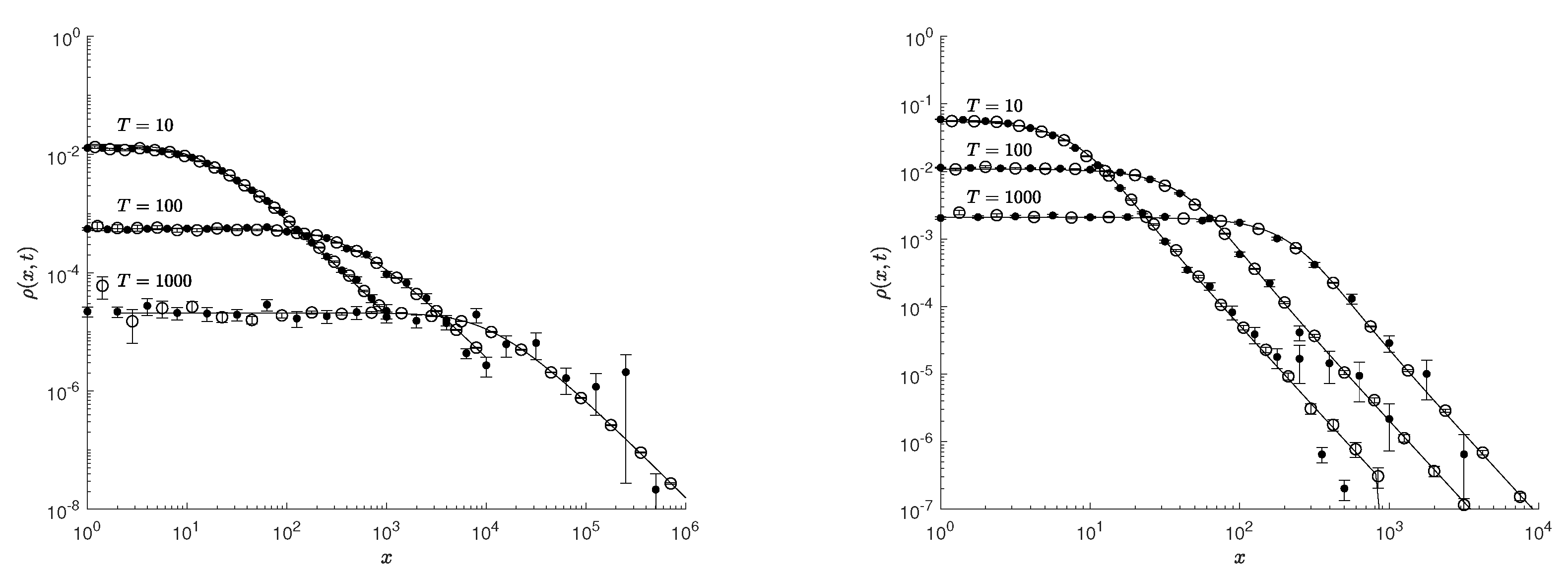
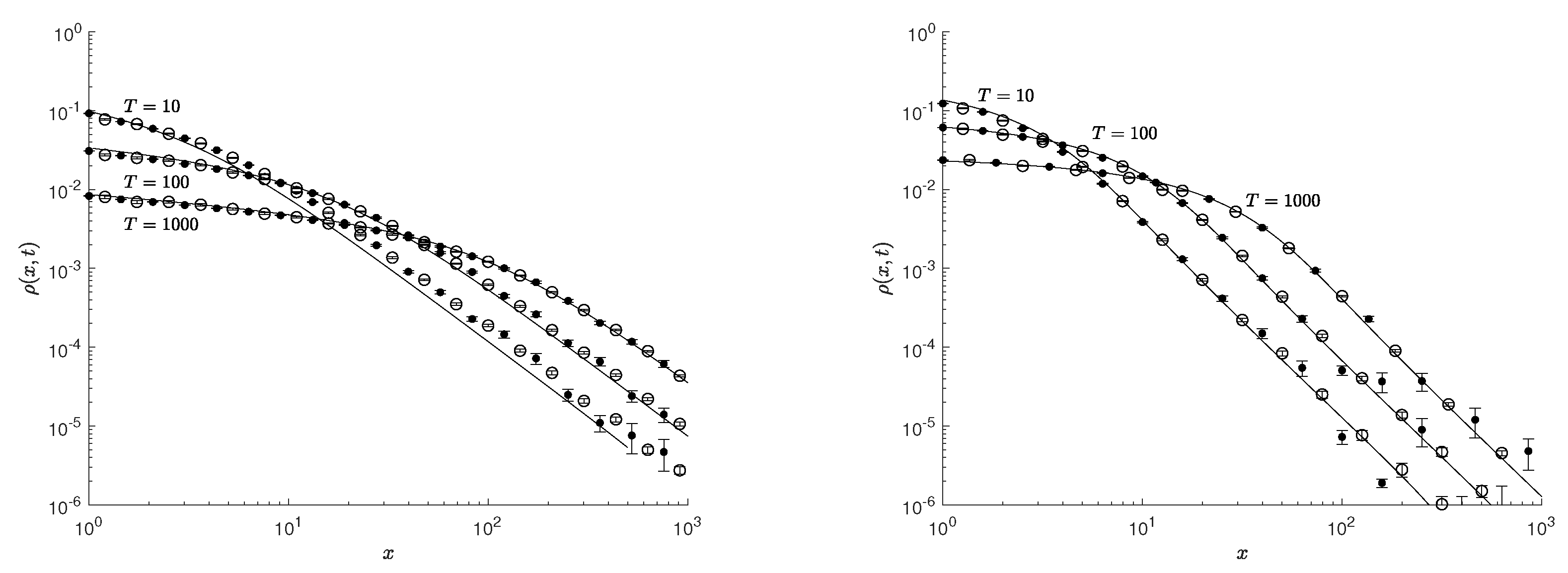
The results of solving Equation (
46) are given in
Figure 1,
Figure 2 and
Figure 3. In these figures, the points correspond to the results of the local estimation (
52), the circles correspond to the results of the histogram estimation (
50), and the solid curves correspond to the solution (
48) with the corresponding diffusion coefficient determined from the relation (
47). The solution results are given for different points in time. From
Figure 1, it is clear that for the parameter value
, the results of the local and histogram estimation coincide with the solution (
48) at time
. This means that by this time, the walk process has already entered the asymptotic regime. Thus, for the given parameter values, the estimate (
52) can be used to solve Equation (
46) at times
. In the case
with the time values
and 100, it is clear (see
Figure 1 on the right) that the results of the local estimate and solution (
48) differ. This means that at such times, the random walk process has not yet reached the asymptotic regime. However, at times
and
, the random walk process already reaches the asymptotic regime. This means that at times
, the estimate (
52) can be used to solve numerically Equation (
46) for the given parameter values. Similar conclusions can be drawn for other presented solution results. For an exponential distribution of rest times and
and
(
Figure 2), it is clear that the random walk process reaches the asymptotic regime at time
. Thus, for the indicated values of the parameters, the estimate (
52) can be used to solve Equation (
46) at times
. In the case
and
(see
Figure 3 on the left), the random walk process becomes asymptotic at time
, and for the values
,
(see
Figure 3 on the right) at time
.
5. Conclusions
The use of the theory of anomalous diffusion and equations in fractional derivatives to describe combustion processes is only at the initial stage of research. At the moment, there are not many papers in which this approach is used to describe combustion processes. However, existing experimental studies (see, for example [
37]) indicate the legitimacy of this approach. One of the main difficulties in using equations in fractional derivatives is finding their solutions. Analytical methods for solving equations of this kind are only at the stage of development. Therefore, one of the main methods of solving equations in fractional derivatives is finite difference methods. In the papers [
41,
42,
43,
44,
45], the numerical solution of the equation of anomalous diffusion is investigated, which is expressed in terms of derivatives of fractional order only in the case when one of the derivatives (or derivative with respect to time or derivative with respect to coordinate) is not of integer order. In this paper, we propose a numerical method for solving the anomalous diffusion equation in which both the time derivative and the coordinate derivative can be of non-integer order.
This paper considers the numerical method for solving the anomalous diffusion equation based on the use of a local estimate. This method is based on the idea of modeling random realizations of particle trajectories. However, unlike the histogram method for estimating the distribution density, each individual trajectory contributes to the estimate not once, but several times. In the proposed approach, after each act of a change in the state of a particle, the probability is calculated that to get to a given point with the coordinate
in a moment of time
, the following collision will turn out to be the final. For the considered model of walks, this probability has the form (
51). This local estimate has several advantages over the histogram estimate. Since the density is estimated at a given point
, then this means that the result of the estimate does not contain a systematic component of the error
. Specifying a set of points
,
, it becomes possible to estimate the solution at several points at once. Moreover, one trajectory will contribute to all points at once
. As a result, the probability
, determined by (
51), is calculated after each act of changing the state of a particle; then, this leads to a considerable decrease in statistical error. Taking account of the fact that from one trajectory, the contribution can be calculated at once to all points
,
of a given set, this means that the desired solution can be constructed as a smooth function of the coordinate
x.
In conclusion, one more important point should be noted. As shown in this study, the equation of anomalous diffusion (
46) describes the asymptotic distribution (at
) of particles in the CTRW process. A characteristic feature of this process is that the random rest times of a particle are characterized by a distribution with an infinite mathematical expectation
, and the random free paths in the case of the exponent
are characterized by an infinite second moment
, and in the case of the exponent value
, then by the infinite mathematical expectation
. Taking into account that in the process of CTRW, a particle instantly moves from one point in space to another (instantaneous jumps), this leads to a non-physical result: in an arbitrarily small time interval, a particle can be at an arbitrarily large distance from the point of its previous position. It should be noted that the random walk process is also characterized by instantaneous jumps that leads to the diffusion Equation (
33). However, as it was shown at the beginning of
Section 3, to obtain normal diffusion, it is necessary to assume that the distributions of the rest time and the distribution of the jump value of a particle have a finite mathematical expectation and a finite variance. As a result, the instantaneous motion of a particle from one point in space to another is compensated by the small value of these jumps. In the case of a power-law distribution of the jump value (
38), the probability of large jumps remains significant for any jump value. As the value decreases of
, this probability increases. This property is characteristic of power distributions. Therefore, when using the equation of anomalous diffusion (
46) to describe combustion processes, especially in furnaces where the geometry is given, a certain amount of care must be taken. It should be understood that the solution to the anomalous diffusion equation decreases according to a power law at
and is different from zero in the entire space. The latter means that the probability of detecting a particle at an arbitrarily large distance from the source at an arbitrarily close moment of time to the initial time is different from zero. Taking account of the fact that this probability decreases according to a power law, then this probability will be significant, and it can no longer be neglected.


 ,
, 


