A Derivative-Free Line-Search Algorithm for Simulation-Driven Design Optimization Using Multi-Fidelity Computations

Abstract

The paper presents a multi-fidelity extension of a local line-search-based derivative-free algorithm for nonsmooth constrained optimization (MF-CS-DFN). The method is intended for use in the simulation-driven design optimization (SDDO) context, where multi-fidelity computations are used to evaluate the objective function. The proposed algorithm starts using low-fidelity evaluations and automatically switches to higher-fidelity evaluations based on the line-search step length. The multi-fidelity algorithm is driven by a suitably defined threshold and initialization values for the step length, which are associated to each fidelity level. These are selected to increase the accuracy of the objective evaluations while progressing to the optimal solution. The method is demonstrated for a multi-fidelity SDDO benchmark, namely pertaining to the hull-form optimization of a destroyer-type vessel, aiming at resistance minimization in calm water at fixed speed. Numerical simulations are based on a linear potential flow solver, where seven fidelity levels are used selecting systematically refined computational grids for the hull and the free surface. The method performance is assessed varying the steplength threshold and initialization approach. Specifically, four MF-CS-DFN setups are tested, and the optimization results are compared to its single-fidelity (high-fidelity-based) counterpart (CS-DFN). The MF-CS-DFN results are promising, achieving a resistance reduction of about 12% and showing a faster convergence than CS-DFN. Specifically, the MF extension is between one and two orders of magnitude faster than the original single-fidelity algorithm. For low computational budgets, MF-CS-DFN optimized designs exhibit a resistance that is about 6% lower than that achieved by CS-DFN.

1. Introduction

Simulation-driven design optimization (SDDO) [1] is an emerging paradigm that offers the possibility to define innovative configurations and optimized designs of complex engineering systems, integrating in a rigorous mathematical framework physics-based computations with numerical optimization algorithms. In many engineering applications, the accuracy of SDDO solutions relies on the use of high-fidelity solvers, which are often computationally expensive. The assessment and optimization of the design performance in realistic operating and environmental conditions, which are always permeated with stochasticity, require computational efforts that can be unattainable for most users. To give an example, recent research showed how an accurate Unsteady Reynolds Averaged Navier–Stokes simulation to evaluate the statistically significant performance of ship maneuvering in irregular waves may require up to 1M CPU hours on HPC systems [2].

In order to reduce the computational cost associated to SDDO, several methodologies have been introduced, integrated, and succesfully applied to complex engineering problems, see e.g., [3]. Methods to reduce the computational cost include linear [4] and nonlinear [5] approaches to design-space dimensionality reduction, adaptive surrogate modeling [6], efficient optimization algorithms [7], and multi-fidelity optimization approaches [8]. Namely, multi-fidelity methods leverage on a fidelity spectrum of computational models (from low to high fidelity), with the objective of maximizing the model accuracy while minimizing the associated computational cost [9,10]. The fidelity spectrum may stem from using different physical models [11,12], spatial and/or time discretizations (e.g., grid size and time step) [13,14,15,16], multidisciplinary coupling (e.g., one- or two-way, tight or loose coupling, etc.) [17,18], degree of solution convergence [19,20], model dimensionality [21,22], and a combination of experimental and numerical data [23,24].

In many (or even most) cases, multi-fidelity methods use surrogate models to fuse information made available by multi-fidelity computations of the design performance [25]. Surrogate-based optimization methods may be classified as either global or local approaches. Global methods, such as polynomial chaos [26], Gaussian processes [27], and radial basis functions [28], provide a global representation of design objectives (and constraints, if required) in the entire design space. This may be achieved by modeling suitable bridge functions (additive, multiplicative, or hybrid additive-multiplicative) [10,29,30] between hierarchical fidelity levels. Then, the resulting global multi-fidelity surrogate is explored by global optimization algorithms. The design optimization and surrogate model training may or may not be integrated using adaptive sampling procedures [31], including resource-[32] and domain-[33] aware approaches to active learning. Local methods such as trust region [34,35] and local surrogate [16] methods fuse multi-fidelity information to provide accurate local approximations of design objectives/constraints (and possibly their derivatives). Local optimization algorithms drive the search for the optimum using the multi-fidelity local model, managing iteratively the trust region center, radius, and model construction, until convergence is achieved [34]. An example is provided in [36], where a unified multi-fidelity quasi-Newton approach is presented that identifies search directions from high-fidelity data, and uses multi-fidelity local models to perform line searches. The method is applied to analytic test problems in [36] and to aero-structural design optimization in [37]. Surrogate-based methods are very promising and have shown their efficiency and effectiveness. Nevertheless, in some cases their training can be costly and their accuracy may decrease (or even drop) as objectives and constraints become noisy or discontinuous, or the number of design variables becomes large [8].

For these reasons, surrogate-free multi-fidelity optimization methods may be used as viable alternatives to surrogate-based methods.

In [38,39] a grid-search algorithm is applied in combination with electromagnetic simulations using spatial grids of variable resolution. The optimization starts on the coarsest spatial grid and is iterated over refined grids. Surrogate models are not used until the finest grid is adopted. Surrogate-free multi-fidelity optimization methods for engineering applications are still little discussed and are worthy of further investigation.

The objective of the present work is the extension of the local line-search-based derivative-free algorithm for nonsmooth constrained optimization (CS-DFN) [40] to multi-fidelity computations without involving surrogate models. The algorithm automatically selects the fidelity to use for the objective function evaluation, based on an internal step-length parameter. Namely, starting from the lowest fidelity, the proposed method moves to higher fidelities as the line-search step length converges to a given threshold.

The method is assessed using an SDDO benchmark pertaining to the hull-form optimization of a destroyer-type vessel in calm water. The benchmark is taken from the NATO Science and Technology Organization, Applied Vehicle Technology, Research Task Group 331 on “Goal-Driven, Multi-Fidelity Approaches for Military Vehicle System-Level Design” [8]. The optimization aims at reducing the ship total resistance at fixed speed and even keel condition. Shape modifications are based on 14 design parameters, modifying globally the hull geometry. The resistance is evaluated by a potential flow solver [41]. Seven fidelity levels are used, which are defined by seven computational grids (spatial discretization). Four algorithmic setups are assessed, where different setups identify different step-length convergence thresholds and reinitialization values. Finally, the proposed multi-fidelity method is compared to its single-fidelity counterpart.

The remainder of the paper is organized as follows. Section 2 introduces the multi-fidelity algorithm. Section 3 describes the SDDO benchmark problem. The numerical results are discussed in Section 4 and, finally, the conclusions are discussed in Section 5.

2. Multi-Fidelity Linesearch-Based Derivative-Free Approach for Nonsmooth Constrained Optimization Algorithm

The proposed algorithm extends the CS-DFN algorithm [40] to the multi-fidelity context, which is here denoted as MF-CS-DFN.

Consider the single-objective and bound-constrained minimization problem

$$\begin{array}{cc}\hfill \mathrm{minimize}& f\left(\mathbf{x}\right)\hfill \\ \hfill \mathrm{subject}\mathrm{to}& \mathbf{x}\in X,\hfill \end{array}$$

(1)

where

$$X=\{\mathbf{x}\in {\mathbb{R}}^N:{\mathbf{x}}_l\le \mathbf{x}\le {\mathbf{x}}_u\}$$

(2)

is a compact set of bound constraints (the domain lower ${\mathbf{x}}_l$ and upper ${\mathbf{x}}_u$ bounds are both finite) for the variables $\mathbf{x}\in {\mathbb{R}}^N$, with N being the number of variables, and the objective function $f\left(\mathbf{x}\right)$ being Lipschitz continuous.

The MF-CS-DFN method described in Algorithm 1 follows an iterative four-step procedure: (1) explores the i-th coordinate direction ${\mathbf{e}}^i$ with a tentative steplength ${\tilde{\alpha }}^i$, evaluates the objective function with the r-fidelity level ${\pi }_r$; (2) the Continuous Search (CS) procedure (see Algorithm 2) [42,43] is used to identify a step length ${\alpha }^i$ that can guarantee a sufficient reduction of the objective function along the ${\mathbf{e}}^i$ direction; (3) provided that the actual (${\alpha }^i$) and tentative (${\tilde{\alpha }}^i$) step lengths are smaller than a given threshold $\eta >0$, a further direction $\mathbf{d}$ is explored through the Projected Continuous Search (PCS) procedure (see Algorithm 3); and (4) if the step lengths in all directions are all below $\eta$ and the r-fidelity is not the highest, the fidelity is increased and the step lengths are reinitialized. The process, starting from the lowest fidelity level, is repeated until the convergence of the algorithm is achieved with the highest fidelity available.

2.1. Continuous Search

The CS takes as inputs the tentative step length ${\tilde{\alpha }}^i$, the current point $\mathbf{y}$, and a direction $\mathbf{p}$ and returns as outputs the actual step $\alpha$ and the computed direction ${\mathbf{p}}_{out}$, which is equal to $\pm \mathbf{p}$. The procedure explores a direction $\mathbf{p}$ searching for the largest $\alpha$ such that sufficient decrease is obtained at point $\mathbf{y}+\alpha \mathbf{p}$. If direction $\mathbf{p}$ cannot provide a sufficient decrease, then the opposite direction is tested before declaring a failure, thus returning the null step $\alpha =0$. When the null step size is returned after the exploration of direction $d^i$, the method decreases the tentative step for the next iteration, i.e., ${\tilde{\alpha }}_{new}^i=\theta {\tilde{\alpha }}_i$, $\theta \in (0,1)$. Otherwise, the tentative step for the next iteration is possibly augmented by setting ${\tilde{\alpha }}_{new}^i=\alpha$.

2.2. Projected Continuous Search

The PCS carries out an exploration along direction $\mathbf{p}$ (or $-\mathbf{p}$ if needed). However, since the direction $\mathbf{p}=\mathbf{d}$ used by the PCS is not equal to $\pm {\mathbf{e}}^i$ for some $i\in \{1,\dots ,N\}$, projections onto X must be taken to ensure feasibility of the generated points. Then, given the current point $\mathbf{y}$ at step k, the procedure first evaluates the function at ${[\mathbf{y}\pm \tilde{\alpha }{\mathbf{d}}_k]}_{[{\mathbf{x}}_l,{\mathbf{x}}_u]}$. In case a sufficient reduction of the function value is obtained, then an extrapolation along the search direction is performed so that a suitable step length $\alpha$ is computed, and it is used as a tentative step length for the next iteration, i.e., ${\tilde{\alpha }}_{new}=\alpha$. On the other hand, if at ${[\mathbf{y}\pm \tilde{\alpha }{\mathbf{d}}_k]}_{[{\mathbf{x}}_l,{\mathbf{x}}_u]}$ a sufficient reduction of the function value is not obtained, then the tentative step length at the next iteration is suitably reduced by a scale factor, i.e., ${\tilde{\alpha }}_{new}=\theta \tilde{\alpha }$, $\theta \in (0,1)$.

Algorithm 1 MF-CS-DFN

Input.$\theta \in (0,1)$, $\xi >0$, $\eta >0$, ${\mathbf{x}}_0\in X$, $\tilde{\alpha }>0$, ${\tilde{\alpha }}^i>0$, ${\mathbf{d}}^i={\mathbf{e}}^i$, for i = 1, …, N such that

$\left|\right|{\mathbf{d}}^i\left|\right|=1$

Let ${\pi }_1,\dots ,{\pi }_r$ with $r\ge 1$ be the precision levels, such that ${\pi }_{i+1}<{\pi }_i$, $i=1,\dots ,r-1$

Set $\overline{j}\leftarrow 1$ and $\mathbf{x}\leftarrow {\mathbf{x}}_0$

for$k=0,1,\dots$do                                                                                 ▹ Start the iterations

Set $\mathbf{y}\leftarrow \mathbf{x}$

for $i=1,\dots ,N$ do

Compute $\alpha$ and ${\mathbf{d}}_{new}^i$ by the Continuous Search (${\tilde{\alpha }}^i$, $\mathbf{y}$, ${\mathbf{d}}^i$; $\alpha$, ${\mathbf{d}}_{new}^i$)           ▹ Call CS

if ($\alpha =0$) then

Set ${\tilde{\alpha }}_{new}^i=\theta {\tilde{\alpha }}^i$

else

Set ${\tilde{\alpha }}_{new}^i=\alpha$

Set ${\alpha }^i\leftarrow \alpha$, ${\mathbf{d}}^i\leftarrow {\mathbf{d}}_{new}^i$, $\mathbf{y}\leftarrow \mathbf{y}+\alpha {\mathbf{d}}_{new}^i$

if (${max}_{i=1,\dots ,n}\{{\alpha }^i,{\tilde{\alpha }}^i\}\le \xi$) then

Compute $\alpha$ and $\tilde{\mathbf{d}}$ by the Projected Continuous Search$(\tilde{\alpha },\mathbf{y},{\mathbf{d}}_k;\alpha ,\tilde{\mathbf{d}})$        ▹ Call PCS

if ($\alpha =0$) then

${\tilde{\alpha }}_{new}=\theta \tilde{\alpha }$

else

${\tilde{\alpha }}_{new}=\alpha$ and $\mathbf{y}\leftarrow {[\mathbf{y}+\alpha \tilde{\mathbf{d}}]}_{[{\mathbf{x}}_l,{\mathbf{x}}_u]}$

else

Set ${\tilde{\alpha }}_{new}=\tilde{\alpha }$

if (${max}_{i=1,\dots ,n}\{{\alpha }^i,{\tilde{\alpha }}^i\}\le \eta$ and $\overline{j}<r$) then

$\overline{j}\leftarrow \overline{j}+1$                                                                       ▹ Increase the accuracy

Set ${\tilde{\alpha }}^i\leftarrow {\tilde{\alpha }}_{new}$, for $i=1,\dots ,N$

Find $\mathbf{x}\in X$ such that $f_{{\pi }_{\overline{j}}}\left(\mathbf{x}\right)\le f_{{\pi }_{\overline{j}}}\left(\mathbf{y}\right)$

Algorithm 2 Continuous Search ($\tilde{\alpha }$, $\mathbf{y}$, $\mathbf{p}$; $\alpha$, ${\mathbf{p}}_{out}$)

Data.$\gamma >0$, $\delta \in (0,1)$

Step 1. Compute the largest $\overline{\alpha }$ such that $\mathbf{y}+\overline{\alpha }\mathbf{p}\in X$. Set $\alpha =min\{\overline{\alpha },\tilde{\alpha }\}$

Step 2. If$\alpha >0$ and $f_{{\pi }_{\overline{j}}}(\mathbf{y}+\alpha \mathbf{p})\le f_{{\pi }_{\overline{j}}}\left(\mathbf{y}\right)-\gamma {\alpha }^2$ then set ${\mathbf{p}}_{out}=\mathbf{p}$ and go to Step 6

Step 3. Compute the largest $\overline{\alpha }$ such that $\mathbf{y}-\overline{\alpha }\mathbf{p}\in X$. Set $\alpha =min\{\overline{\alpha },\tilde{\alpha }\}$

Step 4. If$\alpha >0$ and $f_{{\pi }_{\overline{j}}}(\mathbf{y}-\alpha \mathbf{p})\le f_{{\pi }_{\overline{j}}}\left(\mathbf{y}\right)-\gamma {\alpha }^2$ then set ${\mathbf{p}}_{out}=-\mathbf{p}$ and go to Step 6

Step 5. Set $\alpha =0$, return $\alpha$ and ${\mathbf{p}}_{out}=\mathbf{p}$

Step 6. Let $\beta =min\{\overline{\alpha },(\alpha /\delta )\}$

Step 7. If$\alpha =\overline{\alpha }$ or $f_{{\pi }_{\overline{j}}}(\mathbf{y}+\beta {\mathbf{p}}_{out})>f_{{\pi }_{\overline{j}}}\left(\mathbf{y}\right)-\gamma {\beta }^2$ return $\alpha$ and ${\mathbf{p}}_{out}$

Step 8. Set $\alpha =\beta$ and go to Step 6

Algorithm 3 Projected Continuous Search ($\tilde{\alpha },\mathbf{y},\mathbf{p};\alpha ,{\mathbf{p}}_{out}$)

Data.$\gamma >0$, $\delta \in (0,1)$

Step 0. Set $\alpha =\tilde{\alpha }$

Step 1. If$f_{{\pi }_{\overline{j}}}({[\mathbf{y}+\alpha \mathbf{p}]}_{[{\mathbf{x}}_l,{\mathbf{x}}_u]})\le f_{{\pi }_{\overline{j}}}\left(\mathbf{y}\right)-\gamma {\alpha }^2$then set ${\mathbf{p}}_{out}=\phantom{-}\mathbf{p}$ and go to Step 4

Step 2. If$f_{{\pi }_{\overline{j}}}({[\mathbf{y}-\alpha \mathbf{p}]}_{[{\mathbf{x}}_l,{\mathbf{x}}_u]})\le f_{{\pi }_{\overline{j}}}\left(\mathbf{y}\right)-\gamma {\alpha }^2$then set ${\mathbf{p}}_{out}=-\mathbf{p}$ and go to Step 4

Step 3. Set $\alpha =0$, return $\alpha$ and ${\mathbf{p}}_{out}=\mathbf{p}$

Step 4. Let $\beta =\alpha /\delta$

Step 5. If$f_{{\pi }_{\overline{j}}}({[\mathbf{y}+\beta {\mathbf{p}}_{out}]}_{[{\mathbf{x}}_l,{\mathbf{x}}_u]})>f_{{\pi }_{\overline{j}}}\left(\mathbf{y}\right)-\gamma {\beta }^2$return$\alpha ,{\mathbf{p}}_{out}$

Step 8. Set $\alpha =\beta$ and go to Step 4

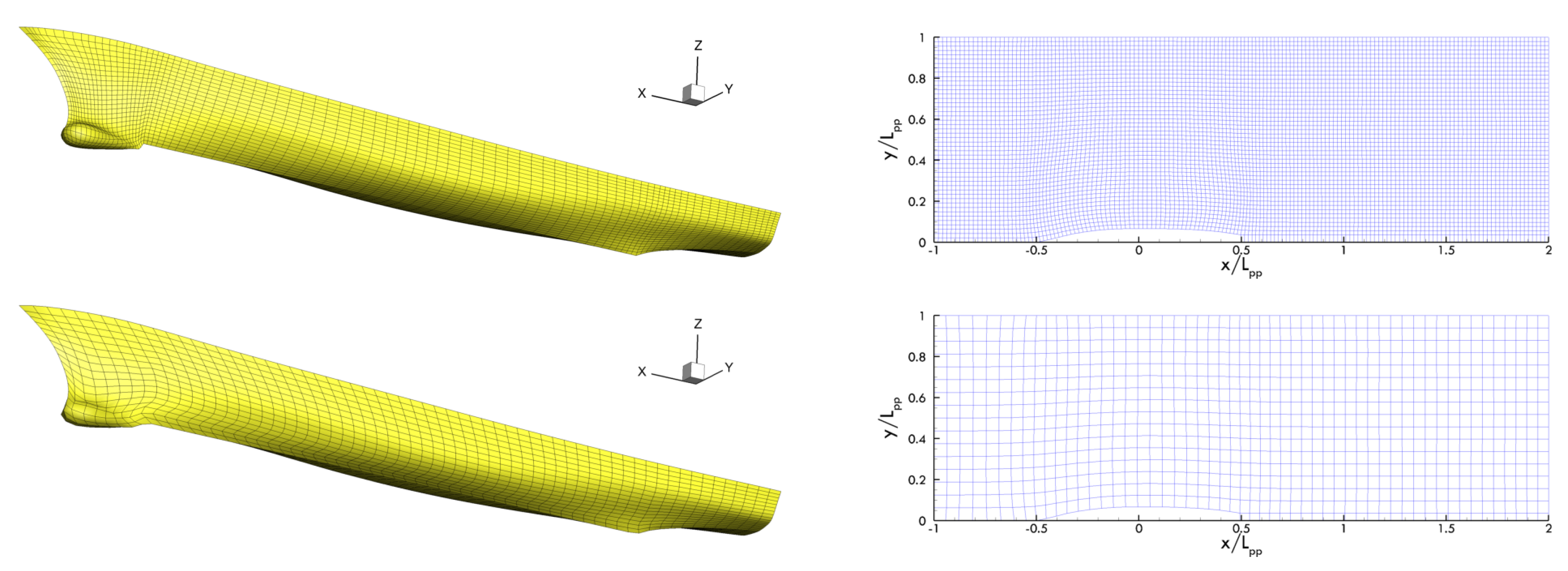
3. SDDO Benchmark Problem

The SDDO benchmark pertains to the total resistance (R) reduction of a destroyer-type vessel in calm water at fixed speed, corresponding to a Froude number (Fr) equal to 0.28. Specifically, the hull under investigation is the DTMB 5415 model, which is a vessel that is extensively used as a benchmark for experimental [44] and computational fluid dynamics [45] as well as for shape optimization problems [46]. The current optimization problem has been defined within the activities of the NATO Science and Technology Organization, Research Task Group-Applied Vehicle Technology 331 on “Goal-Driven, multi-fidelity approaches for military vehicle system-level design” [8], and it reads

$$\begin{array}{c}\hfill \begin{array}{cc}\hfill \mathrm{minimize}& \mathsf{\Delta }R\left(\mathbf{x}\right)/R_0\mathrm{with}\mathbf{x}\in {\mathbb{R}}^N\hfill \\ \hfill \mathrm{subject}\mathrm{to}& L_{\mathrm{pp}}\left(\mathbf{x}\right)=L_{{\mathrm{pp}}_0}\hfill \\ \hfill \mathrm{and}\mathrm{to}& \nabla \left(\mathbf{x}\right)={\nabla }_0\hfill \\ & \left|\mathsf{\Delta }B\left(\mathbf{x}\right)\right|\le 0.05B_0\hfill \\ & \left|\mathsf{\Delta }T\left(\mathbf{x}\right)\right|\le 0.05T_0\hfill \\ & V\left(\mathbf{x}\right)\ge V_0\hfill \\ & -1\le x_i\le 1\mathrm{with}\forall i=1,\dots ,N\hfill \end{array}\end{array}$$

(3)

where $\mathsf{\Delta }R\left(\mathbf{x}\right)=R\left(\mathbf{x}\right)-R_0$, $\mathbf{x}$ collects the design variables, $L_{\mathrm{pp}}$ is the length between perpendiculars, ∇ is the ship displacement (volume of water displaced), B is the overall beam, T is the drought, and V is the volume reserved for the sonar in the bow dome. Subscript “0” indicates parent (original) hull values. Equality and inequality constraints for the geometry deformations are taken from [46].

Table 1. DTMB 5415 original hull main particulars and simulation conditions.

Quantity	Symbol	Unit	Value
Displacement	∇	m3	0.549
Length between perpendiculars	$L_{\mathrm{pp}}$	m	5.720
Beam	B	m	0.760
Draft	T	m	0.248
Water density	$\rho$	kg/m3	998.5
Kinematic viscosity	$\nu$	m2/s	1.09 × 106
Gravity acceleration	g	m/s2	9.803
Froude number	Fr	–	0.280

summarizes the main characteristics of the hull and simulation conditions for the hydrodynamic solver. The latter, developed at the CNR-INM [41], is based on the Dawson linearization [47] of the potential flow equations. The total resistance is estimated as the sum of the wave and the frictional resistance. The wave component is evaluated using the pressure integral over the hull surface, whereas the frictional component is estimated using a flat-plate approximation based on the local Reynolds number [48].

Finally, the design space is composed by $N=14$ design variables, defining the shape modifications. These are based on a linear superposition on the computational hull-surface grid of a set of orthonormal functions, coming from a physics-informed design-space dimensionality reduction procedure [49]. It may be noted that the design variables and the associated shape modifications are organized in a hierarchical order, meaning that the first variables produce larger design modifications than the last ones. For further details, the interested reader is referred to [3].

The multi-fidelity levels are defined by the computational grid size. Specifically, the benchmark is defined with seven grid (fidelity) levels with a refinement ratio of 2^0.25, as an example the finest (G1) and coarsest (G7) grids are shown in Figure 1.

Table 2. Fidelity levels details: grid size, resistance, associated error ($E_G$), and normalized computational cost (NCC).

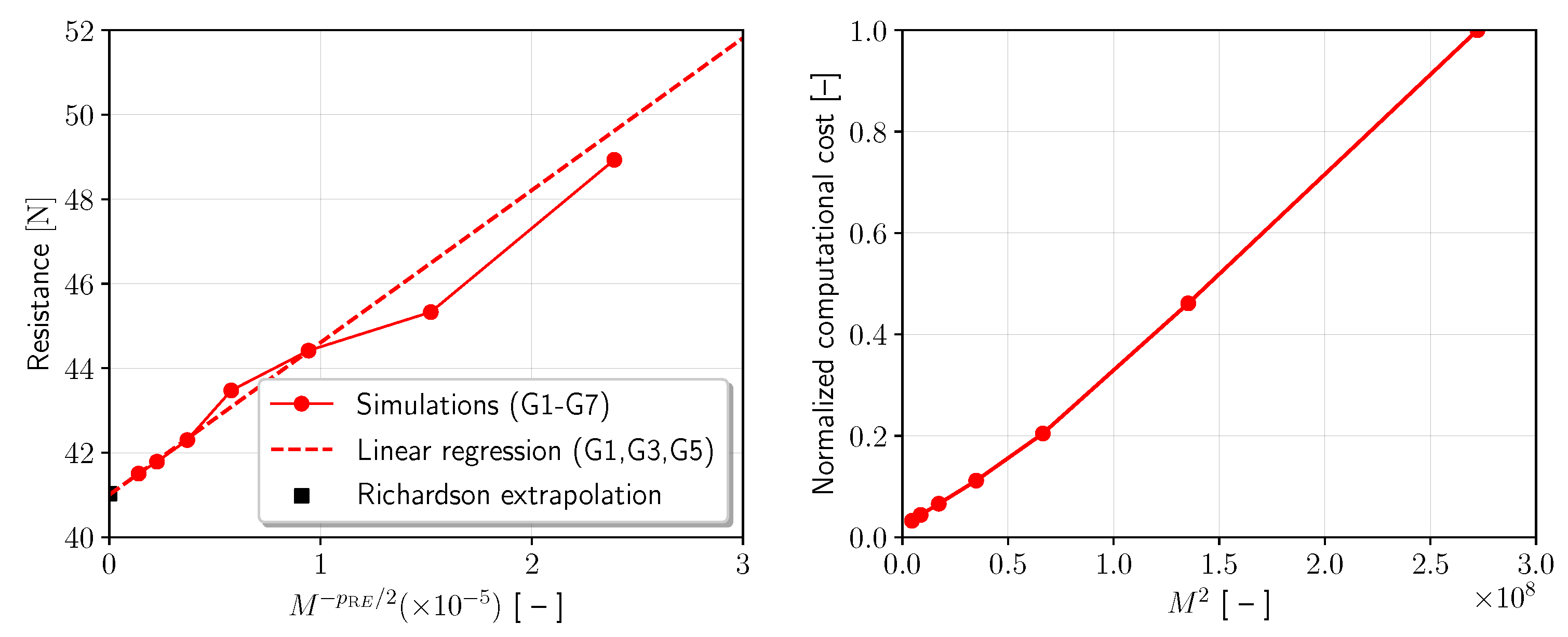
Grid	Hull Nodes	Free-Surface Nodes	Total Nodes (M)	Resistance [N]	Grid Error (${\mathit{E}}_{\mathit{G}}$%)	NCC
G1	$150\times 50$	$180\times 50$	16.5k	41.5	1.16	1.00
G2	$126\times 42$	$151\times 42$	11.6k	41.8	1.85	0.46
G3	$106\times 35$	$127\times 35$	8.2k	42.3	3.10	0.20
G4	$89\times 29$	$107\times 29$	5.7k	43.5	5.97	0.11
G5	$76\times 25$	$90\times 25$	4.2k	44.4	8.26	0.07
G6	$64\times 21$	$76\times 21$	2.9k	45.3	10.5	0.04
G7	$54\times 18$	$64\times 18$	2.1k	48.9	19.3	0.03

Note: refinement ratio equal to 2^0.25.

summarizes the grid sizes, along with the associated nodes number (M), the resistance computed for the original hull ($R_0$), an estimate of the grid error ($E_G$, see below), and the normalized computation cost (NCC). The NCC is evaluated as the ratio between the CPU time needed for a simulation with the generic j-th fidelity and the highest-fidelity. Figure 2 shows the convergence of the resistance estimate as a function of the grid/fidelity level and the associated computational cost. Pressure on the hull and wave elevation patterns are shown in Figure 3. Moving from the highest (G1) to the lowest (G7) fidelity, a lower pressure is predicted on the hull aft and, overall, there are smaller pressure gradients along the hull. Furthermore, the wave elevation decreases and the diverging bow waves are less evident. The linear regression based on G1, G3, and G5 triplet (see Figure 2, left) converges to the solution given by the Richardson extrapolation [50], which provides an order of convergence of the numerical solver equal to $p_{\mathrm{RE}}\approx 2.8$. All the fidelities lie close to the regression, and the associated grid errors $E_G$ are evaluated with respect to the Richardson extrapolation value. For the sake of simplicity, this error is considered constant within the design space. Finally, Figure 2 (right) shows how the NCC scales near linearly with the square of the grid size.

The current benchmark problem is available as open-source Fortran code at the following GitHub repository: github.com/MAORG-CNR-INM/NATO-AVT-331-L2-Sea-Benchmark.

4. Numerical Results

In this paper, the implementation of MF-CS-DFN uses the following values for the constants

$$\theta =0.5,\xi ={10}^{-3},{\mathbf{x}}_0=\mathbf{0},\gamma ={10}^{-4},\delta =0.5.$$

(4)

where $\mathbf{0}$ denotes the all-zero vector with 14 components. It should be noted that the MF-CS-DFN performance is affected by the step length $\tilde{\alpha }$ and the convergence threshold $\eta$, see Algorithm 1. Therefore, a parametric analysis is performed investigating the combination of static/dynamic steplength threshold and reinitialization. Specifically, the use of a dynamic approach aims at defining an adaptive setup to the specific characteristics of the problem at hand. Four setups of the MF-CS-DFN algorithm are tested. For each setup, a combination of the steplength convergence threshold $\eta$ and its reinitialization value ${\tilde{\alpha }}_{new}$ is defined; see

Table 3. MF-CS-DFN setups: steplength threshold and reinitialization values.

		Reinitialization ${\tilde{\mathit{\alpha }}}_{\mathbf{new}}$
		Static, 1	Dynamic, $10{\mathit{\alpha }}_{{\mathit{\pi }}_{\overline{\mathit{j}}+\mathbf{1}}}$
Threshold$\mathbf{\eta }$	Static, 10 × 10−3	StSr	StDr
	Dynamic, $E_G$	DtSr	DtDr

.

The performance of MF-CS-DFN using the proposed setups is assessed and compared to its single-fidelity counterpart (CS-DFN) that uses the highest fidelity only. The NCC is used for the convergence analysis.

Figure 4 compares the optimization convergence of MF-CS-DFN and CS-DFN. The resistance reduction is evaluated with respect to the original hull with the grid used during the optimization segment (e.g., when the MF-CS-DFN is using G5, the resistance variation is computed with respect to the original hull evaluated with G5). Note that the MF-CS-DFN results start with a lower initial computational cost since the first evaluation is performed on the lowest-fidelity (G7). The convergence of the MF-CS-DFN shows some changes in the objective function when the algorithm switches computational grids. Specifically, coarse grids overestimate the resistance improvement. Nevertheless, the objective function remains consistently below 0%, meaning that the optimal designs identified with coarse grids are found to reduce the resistance also with fine grids. Except for the use of StDr setups, MF-CS-DFN achieves better optima (larger resistance reduction) than CS-DFN. Furthermore, MF-CS-DFN achieves a larger resistance reduction with a reduced computational cost than CS-DFN. The use of a dynamic approach (Dt setups) to manage the steplength threshold produces better results than using a fixed one (St setups). Furthermore, the use of a static reinitialization (Sr setups) provides better results than Dr for both approaches. Overall, the DtSr setup achieves the best optimum.

Figure 5 shows the optimized variable values. Except for the StDr setup, MF-CS-DFN setups provide similar variable values for $x_1$, $x_2$, and $x_4$. Greater differences can be noted when comparing the other variables. Since the first variables are those that have a more significant effect on the shape modification, all the MF-CS-DFN setups achieve similar optimal hull shapes. Specifically, Figure 6 shows the magnitude of the shape modification for optimal hulls with respect to the parent one. The shape modification is distributed between the bow, mid-length, and aft regions. Overall, the shape modifications provided by the different setups are similar, with only local differences, especially in the aft region.

Figure 7 shows the initial and converged value of the design variables for each fidelity level of MF-CS-DFN (DtSr) in comparison to CS-DFN. Most of the variables converge toward the final value already with the coarser grids (lower fidelities), meaning that the lower fidelities are in good correlation with the highest fidelity level. Overall, the design variable values can be considered very close to convergence already with G3.

Figure 8 compares CS-DFN and MF-CS-DFN (DrSt) convergences, along with the MF-CS-DFN (DrSt) validation (current optimal designs assessed with G1) at each grid change, which is denoted in the plot by vertical dashed lines. Coarse grids resistance reductions are overall in good agreement with G1-validated values, except for G5. It may be noted that G1-validated values of resistance reductions provided by MF-CS-DFN are always lower than those provided by CS-DFN with the same computational cost. Namely, switching from G7 to G6, the resistance significantly reduces, and the G1-validated value is already significantly lower than that provided by CS-DFN. In addition, validated values for NCC > 6 show small improvements, meaning that MF-CS-DFN has already converged to the neighborhood of the final optimum, as also shown in Figure 7. This means that the proposed algorithm converges significantly faster than CS-DFN. Finally, it may be noted that MF-CS-DFN achieves a better solution than CS-DFN with the available computational resources.

Table 4. MF-CS-DFN (DtSr) resistance and its reduction, G1 validation of the resistance reduction, resistance improvement (gain) with respect to the CS-DFN, and cumulative normalized computational cost for each grid.

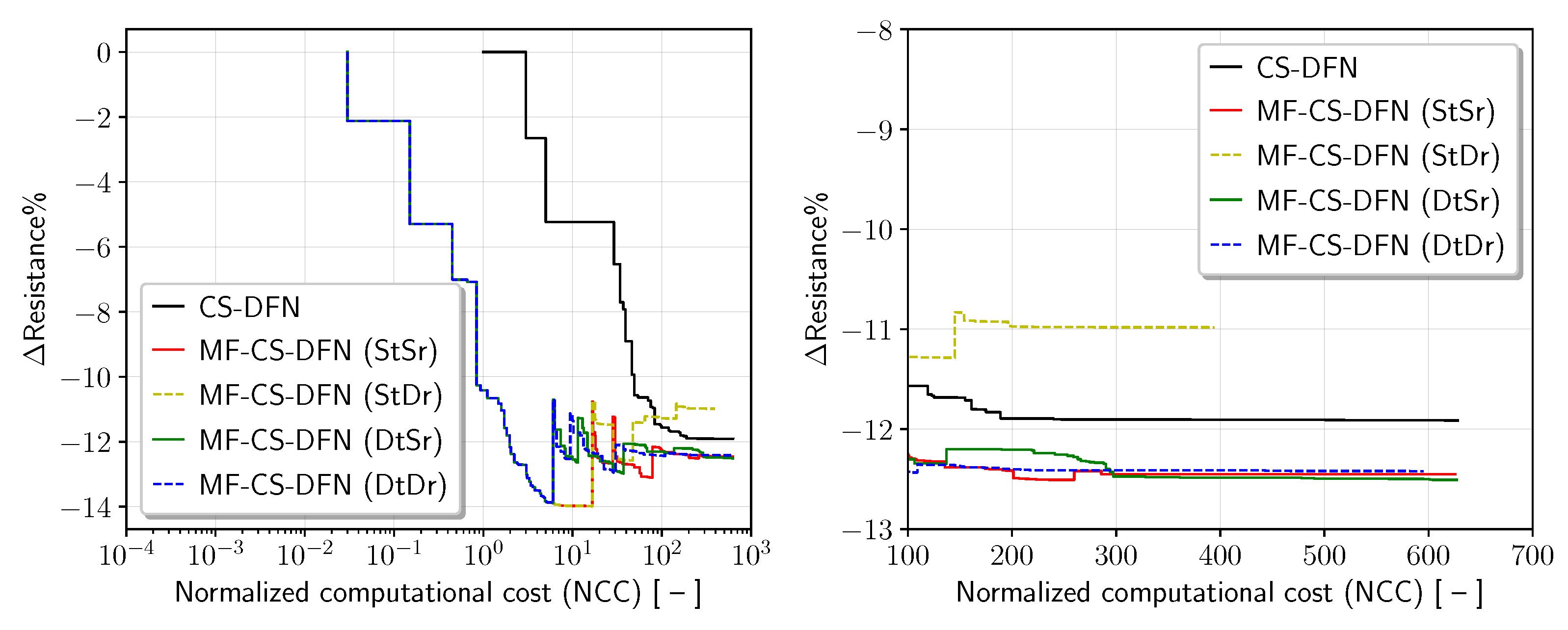
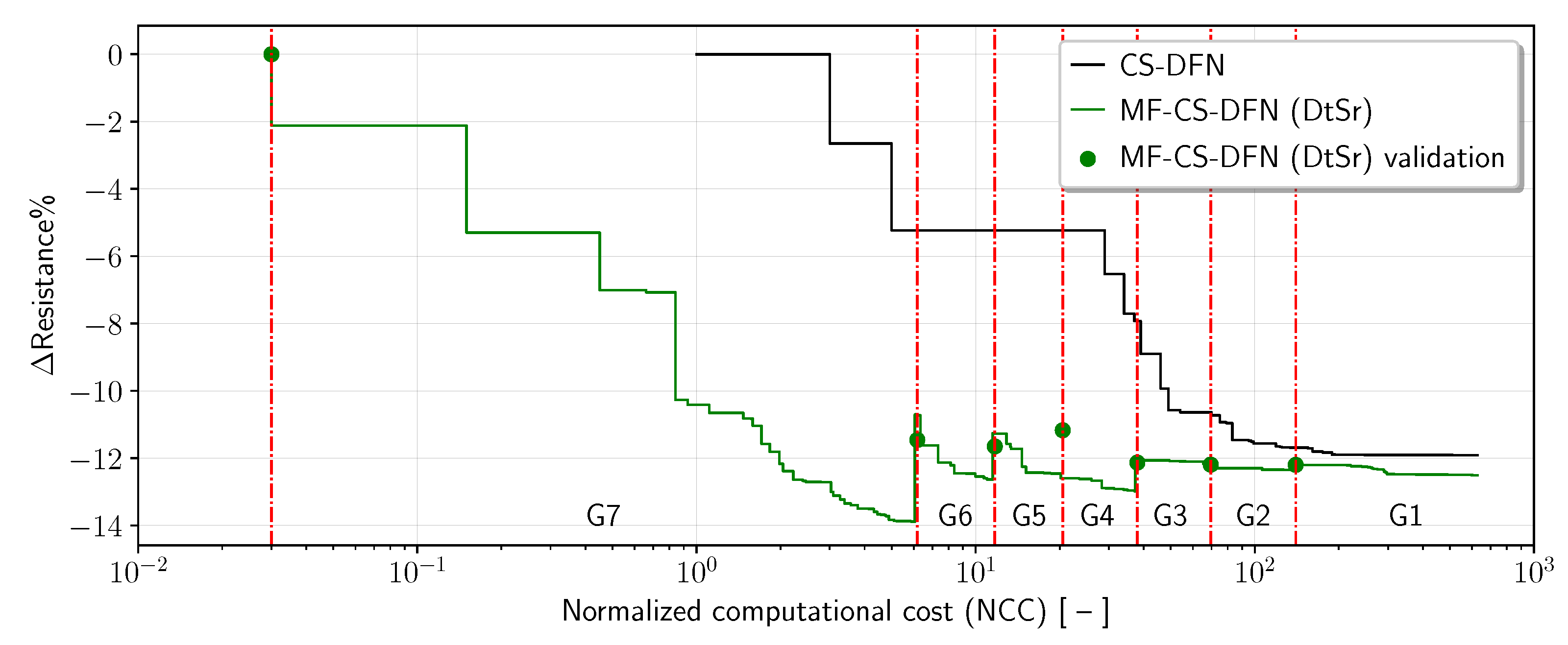
Grid	Optimized ${\mathit{R}}_{\mathit{j}}$ [N]	Optimized $\mathsf{\Delta }{\mathit{R}}_{\mathit{j}}$%	Optimized $\mathsf{\Delta }{\mathit{R}}_1$%	Gain of MF-CS-DFN%	Cumulative NCC [-]
G7	42.1	−13.9	−11.5	6.57	6.18
G6	39.6	−12.6	−11.6	6.77	11.7
G5	38.9	−12.4	−11.2	6.27	20.5
G4	37.8	−13.0	−12.1	4.79	37.9
G3	37.1	−12.2	−12.2	1.74	69.5
G2	36.6	−12.3	−12.2	0.59	140
G1	36.3	−12.5	−12.5	0.67	628

summarizes the MF-CS-DFN results, showing the resistance and its reduction provided by each computational grid, along with the corresponding G1-validated values and the gain of MF-CS-DFN versus CS-DFN for the same computational cost. It may be noted how the gain is significant (6% and above) especially for low computational budgets.

Finally, Figure 9 shows a comparison between the original and the MF-CS-DFN (DtSr) optimal hull. The optimal hull shows a better recovery of the pressure toward the stern and more prominent cavities in the bow and aft regions of the hull, resulting in an overall lower wave elevation of both bow and stern diverging waves.

5. Conclusions

A multi-fidelity extension of the local line-search-based derivative-free approach for nonsmooth constrained optimization (MF-CS-DFN) is introduced for design optimization, which is driven by multi-fidelity computations. The proposed algorithm drives the search for the optimum starting from the lowest fidelity level and then moving to higher fidelities (increasing the accuracy of the numerical solution) as given convergence criteria are met, based on the step length. A simulation-driven design optimization benchmark is used for the algorithm assessment, pertaining to the hull-form optimization of a destroyer-type vessel for total resistance reduction in calm water. Four MF-CS-DFN setups are tested, and the method is compared to its single-fidelity counterpart (CS-DFN). Specifically, static and dynamic thresholds of the step length are considered in combination with its static and dynamic reinitialization. The dynamic threshold is set equal to the error associated to the computational grid used for the resistance evaluation.

Three out of four MF-CS-DFN setups perform better than CS-DFN. MF-CS-DFN converges faster to a lower resistance value (with a lower computational cost) than CS-DFN. Specifically, MF-CS-DFN shows a convergence that is between one and two orders of magnitude faster than the original single-fidelity algorithm. Furthermore, for low computational budgets, the optimized designs with MF-CS-DFN exhibit a resistance that is about 6% lower than that achieved with CS-DFN. In particular, the use of a dynamic threshold for the step length (Dr setups) produces better results than the use of a static threshold. This is because the algorithm efficiently stops using a given fidelity level when this is no longer informative. Finally, the MF-CS-DFN step-length reinitialization has a little influence on the algorithm performance, although a slightly better behavior is observed when it is used statically.

Obviously, the efficiency and efficacy of the algorithm depend on the correlation of the objective function evaluation between different fidelity levels. Moreover, the method is local, providing a local solution to the design optimization problem. We may conclude that provided that subsequent fidelity levels are reasonably correlated to each other and a local solution to the optimization problem is sought after, the MF-CS-DFN is a viable alternatives to surrogate-based methods for multi-fidelity optimization.

References

- Harries, S.; Abt, C. Faster turn-around times for the design and optimization of functional surfaces. Ocean Eng. 2019, 193, 106470. [Google Scholar] [CrossRef]
- Serani, A.; Diez, M.; van Walree, F.; Stern, F. URANS analysis of a free-running destroyer sailing in irregular stern-quartering waves at sea state 7. Ocean Eng. 2021, 237, 109600. [Google Scholar] [CrossRef]
- Serani, A.; Stern, F.; Campana, E.F.; Diez, M. Hull-form stochastic optimization via computational-cost reduction methods. Eng. Comput. 2021, 1–25. [Google Scholar] [CrossRef]
- D’Agostino, D.; Serani, A.; Diez, M. Design-space assessment and dimensionality reduction: An off-line method for shape reparameterization in simulation-based optimization. Ocean Eng. 2020, 197, 106852. [Google Scholar] [CrossRef]
- D’Agostino, D.; Serani, A.; Campana, E.F.; Diez, M. Nonlinear Methods for Design-Space Dimensionality Reduction in Shape Optimization. In Proceedings of the 3rd International Conference on Machine Learning, Optimization, and Big Data, MOD 2017, Volterra, Italy, 14–17 September 2017. [Google Scholar]
- Alizadeh, R.; Allen, J.K.; Mistree, F. Managing computational complexity using surrogate models: A critical review. Res. Eng. Des. 2020, 31, 275–298. [Google Scholar] [CrossRef]
- Jones, D.R.; Martins, J.R. The DIRECT algorithm: 25 years Later. J. Glob. Optim. 2021, 79, 521–566. [Google Scholar] [CrossRef]
- Beran, P.S.; Bryson, D.E.; Thelen, A.S.; Diez, M.; Serani, A. Comparison of Multi-Fidelity Approaches for Military Vehicle Design. In Proceedings of the 21th AIAA/ISSMO Multidisciplinary Analysis and Optimization Conference (MA&O), AVIATION 2020, Denver, CO, USA, 5–9 June 2020. [Google Scholar]
- Giselle Fernández-Godino, M.; Park, C.; Kim, N.H.; Haftka, R.T. Issues in deciding whether to use multifidelity surrogates. AIAA J. 2019, 57, 2039–2054. [Google Scholar] [CrossRef]
- Giselle Fernández-Godino, M.; Park, C.; Kim, N.H.; Haftka, R.T. Review of multi-fidelity models. arXiv 2016, arXiv:1609.07196. [Google Scholar]
- Vanilla, T.T.; Benoit, A.; Benoit, P. Hydro-elastic response of composite hydrofoil with FSI. Ocean Eng. 2021, 221, 108230. [Google Scholar] [CrossRef]
- Anselma, P.; Niutta, C.B.; Mainini, L.; Belingardi, G. Multidisciplinary design optimization for hybrid electric vehicles: Component sizing and multi-fidelity frontal crashworthiness. Struct. Multidiscip. Optim. 2020, 62, 2149–2166. [Google Scholar] [CrossRef]
- Biehler, J.; Gee, M.W.; Wall, W.A. Towards efficient uncertainty quantification in complex and large-scale biomechanical problems based on a Bayesian multi-fidelity scheme. Biomech. Model. Mechanobiol. 2015, 14, 489–513. [Google Scholar] [CrossRef] [PubMed]
- Jonsson, I.M.; Leifsson, L.; Koziel, S.; Tesfahunegn, Y.A.; Bekasiewicz, A. Shape optimization of trawl-doors using variable-fidelity models and space mapping. Procedia Comput. Sci. 2015, 51, 905–913. [Google Scholar] [CrossRef] [Green Version]
- Koziel, S.; Tesfahunegn, Y.; Amrit, A.; Leifsson, L.T. Rapid multi-objective aerodynamic design using co-kriging and space mapping. In Proceedings of the 57th AIAA/ASCE/AHS/ASC Structures, Structural Dynamics, and Materials Conference, San Diego, CA, USA, 4–8 January 2016; p. 0418. [Google Scholar]
- Song, Y.; Cheng, Q.S.; Koziel, S. Multi-fidelity local surrogate model for computationally efficient microwave component design optimization. Sensors 2019, 19, 3023. [Google Scholar] [CrossRef] [Green Version]
- Leotardi, C.; Serani, A.; Iemma, U.; Campana, E.F.; Diez, M. A variable-accuracy metamodel-based architecture for global MDO under uncertainty. Struct. Multidiscip. Optim. 2016, 54, 573–593. [Google Scholar] [CrossRef]
- Volpi, S.; Diez, M.; Stern, F. Multidisciplinary design optimization of a 3D composite hydrofoil via variable accuracy architecture. In Proceedings of the 2018 Multidisciplinary Analysis and Optimization Conference, Atlanta, GA, USA, 25–29 June 2018; p. 4173. [Google Scholar]
- Branke, J.; Asafuddoula, M.; Bhattacharjee, K.S.; Ray, T. Efficient use of partially converged simulations in evolutionary optimization. IEEE Trans. Evol. Comput. 2016, 21, 52–64. [Google Scholar] [CrossRef] [Green Version]
- Palar, P.S.; Zuhal, L.R.; Shimoyama, K.; Tsuchiya, T. Global sensitivity analysis via multi-fidelity polynomial chaos expansion. Reliab. Eng. Syst. Saf. 2018, 170, 175–190. [Google Scholar] [CrossRef] [Green Version]
- Zou, Z.; Liu, J.; Zhang, W.; Wang, P. Shroud leakage flow models and a multi-dimensional coupling CFD (computational fluid dynamics) method for shrouded turbines. Energy 2016, 103, 410–429. [Google Scholar] [CrossRef]
- Le Gratiet, L.; Cannamela, C.; Iooss, B. A Bayesian approach for global sensitivity analysis of (multifidelity) computer codes. SIAM/ASA J. Uncertain. Quantif. 2014, 2, 336–363. [Google Scholar] [CrossRef]
- Kuya, Y.; Takeda, K.; Zhang, X.; Forrester, A.I. Multifidelity surrogate modeling of experimental and computational aerodynamic data sets. AIAA J. 2011, 49, 289–298. [Google Scholar] [CrossRef]
- Choi, W.; Radhakrishnan, K.; Kim, N.H.; Park, J.S. Multi-Fidelity Surrogate Models for Predicting Averaged Heat Transfer Coefficients on Endwall of Turbine Blades. Energies 2021, 14, 482. [Google Scholar] [CrossRef]
- Peherstorfer, B.; Willcox, K.; Gunzburger, M. Survey of multifidelity methods in uncertainty propagation, inference, and optimization. Siam Rev. 2018, 60, 550–591. [Google Scholar] [CrossRef]
- Rumpfkeil, M.P.; Beran, P.S. Multi-Fidelity, Gradient-enhanced, and Locally Optimized Sparse Polynomial Chaos and Kriging Surrogate Models Applied to Benchmark Problems. In Proceedings of the AIAA Scitech 2020 Forum, Orlando, FL, USA, 6–10 January 2020; p. 0677. [Google Scholar]
- Coppedè, A.; Gaggero, S.; Vernengo, G.; Villa, D. Hydrodynamic shape optimization by high fidelity CFD solver and Gaussian process based response surface method. Appl. Ocean Res. 2019, 90, 101841. [Google Scholar] [CrossRef]
- Nuñez, L.; Regis, R.G.; Varela, K. Accelerated random search for constrained global optimization assisted by radial basis function surrogates. J. Comput. Appl. Math. 2018, 340, 276–295. [Google Scholar] [CrossRef]
- Han, Z.H.; Görtz, S.; Zimmermann, R. Improving variable-fidelity surrogate modeling via gradient-enhanced kriging and a generalized hybrid bridge function. Aerosp. Sci. Technol. 2013, 25, 177–189. [Google Scholar] [CrossRef]
- Bryson, D.E.; Rumpfkeil, M.P. All-at-once approach to multifidelity polynomial chaos expansion surrogate modeling. Aerosp. Sci. Technol. 2017, 79, 121–136. [Google Scholar] [CrossRef]
- Liu, H.; Ong, Y.S.; Cai, J. A survey of adaptive sampling for global metamodeling in support of simulation-based complex engineering design. Struct. Multidiscip. Optim. 2018, 57, 393–416. [Google Scholar] [CrossRef]
- Grassi, F.; Manganini, G.; Garraffa, M.; Mainini, L. Resource Aware Multifidelity Active Learning for Efficient Optimization. In Proceedings of the AIAA Scitech 2021 Forum, Nashville, TN, USA, 11–15 January 2021; p. 0894. [Google Scholar]
- Di Fiore, F.; Maggiore, P.; Mainini, L. Multifidelity domain-aware learning for the design of re-entry vehicles. Struct. Multidiscip. Optim. 2021, 64, 3017–3035. [Google Scholar] [CrossRef]
- Alexandrov, N.M.; Dennis, J.; Lewis, R.M.; Torczon, V. A trust-region framework for managing the use of approximation models in optimization. Struct. Optim. 1998, 15, 16–23. [Google Scholar] [CrossRef]
- March, A.; Willcox, K. Provably convergent multifidelity optimization algorithm not requiring high-fidelity derivatives. AIAA J. 2012, 50, 1079–1089. [Google Scholar] [CrossRef] [Green Version]
- Bryson, D.E.; Rumpfkeil, M.P. Multifidelity quasi-newton method for design optimization. AIAA J. 2018, 56, 4074–4086. [Google Scholar] [CrossRef]
- Bryson, D.E.; Rumpfkeil, M.P. Aerostructural Design Optimization Using a Multifidelity Quasi-Newton Method. J. Aircr. 2019, 56, 2019–2031. [Google Scholar] [CrossRef]
- Koziel, S. Computationally efficient multi-fidelity multi-grid design optimization of microwave structures. ACES J.-Appl. Comput. Electromagn. Soc. 2010, 25, 578. [Google Scholar]
- Koziel, S. Multi-fidelity multi-grid design optimization of planar microwave structures with Sonnet. Int. Rev. Prog. Appl. Comput. Electromagn. 2010, 4, 26–29. [Google Scholar]
- Fasano, G.; Liuzzi, G.; Lucidi, S.; Rinaldi, F. A linesearch-based derivative-free approach for nonsmooth constrained optimization. SIAM J. Optim. 2014, 24, 959–992. [Google Scholar] [CrossRef] [Green Version]
- Bassanini, P.; Bulgarelli, U.; Campana, E.F.; Lalli, F. The wave resistance problem in a boundary integral formulation. Surv. Math. Ind. 1994, 4, 151–194. [Google Scholar]
- Lucidi, S.; Sciandrone, M. A Derivative-Free Algorithm for Bound Constrained Optimization. Comput. Optim. Appl. 2002, 21, 119–142. [Google Scholar] [CrossRef]
- Liuzzi, G.; Lucidi, S.; Rinaldi, F. Derivative-free methods for bound constrained mixed-integer optimization. Comput. Optim. Appl. 2012, 53, 505–526. [Google Scholar] [CrossRef] [Green Version]
- Irvine, M., Jr.; Longo, J.; Stern, F. Pitch and Heave Tests and Uncertainty Assessment for a Surface Combatant in Regular Head Waves. J. Ship Res. 2008, 52, 146–163. [Google Scholar] [CrossRef]
- Larsson, L.; Stern, F.; Visonneau, M.; Hirata, N.; Hino, T.; Kim, J. Proceedings, Tokyo 2015 Workshop on CFD in Ship Hydrodynamics. In Proceedings of the Tokyo CFD Workshop, Tokyo, Japan, 2–4 December 2015. [Google Scholar]
- Grigoropoulos, G.; Campana, E.; Diez, M.; Serani, A.; Goren, O.; Sariöz, K.; Danişman, D.; Visonneau, M.; Queutey, P.; Abdel-Maksoud, M.; et al. Mission-based hull-form and propeller optimization of a transom stern destroyer for best performance in the sea environment. In Proceedings of the VII International Conference on Computational Methods in Marine Engineering MARINE 2017, Nantes, France, 15–17 May 2017. [Google Scholar]
- Dawson, C.W. A practical computer method for solving ship-wave problems. In Proceedings of the 2nd International Conference on Numerical Ship Hydrodynamics, Berkeley, CA, USA, 19–21 September 1977; pp. 30–38. [Google Scholar]
- Schlichting, H.; Gersten, K. Boundary-Layer Theory; Springer: Berlin, Germany, 2000. [Google Scholar]
- Serani, A.; Campana, E.F.; Diez, M.; Stern, F. Towards Augmented Design-Space Exploration via Combined Geometry and Physics Based Karhunen-Loève Expansion. In Proceedings of the AIAA-AVIATION 2017 Conference, Denver, CO, USA, 5–9 June 2017. [Google Scholar]
- Xing, T.; Stern, F. Factors of safety for Richardson extrapolation. J. Fluids Eng. 2010, 132, 061403. [Google Scholar] [CrossRef] [Green Version]