Machine Learning Models to Predict Critical Episodes of Environmental Pollution for PM2.5 and PM10 in Talca, Chile

Abstract

One of the main environmental problems that affects people’s health and quality of life is air pollution by particulate matter. Chile has nine of the ten most polluted cities in South America according to a report presented in 2019 by Greenpeace and AirVisual that measured the air quality index based on the levels of fine particles. Most Chilean cities are highly contaminated by particulate matter, especially during the months of April to August (the critical episode management period). The objective of this study is to predict particulate matter levels based on meteorological and climatic features, such as temperature, wind speed, wind direction, precipitation and relative air humidity in Talca, Chile, during the critical episode management periods between 2014 and 2018. Predictive models based on machine learning techniques were used, considering training datasets with meteorological and climatic data, and particulate matter levels from the three air quality monitoring stations in Talca, Chile. We carried out the training of 24 models to predict particulate matter levels considering the 24-h average and average between 05:00 to 11:00 p.m. For the model testing, data from the year 2018 during the critical episode management period were used. The obtained results indicate that our models are able to effectively predict levels of particulate matter, enabling correct management of critical episodes, especially for alert, pre-emergency and emergency conditions. We used the cross-platform and open-source programming language Python for the development and implementation of the proposed models and R-project for some visualizations.

1. Introduction

The increase in air pollution rates, the product of suspended particulate matter (PM), is a constant concern throughout the world that, year after year, impacts human health and quality of life [1]. In Chile, improving air quality has been a government priority for years. Diagnosis of emissions of atmospheric pollutants has been carried out in the main cities of the country, stimulating efforts to reduce the pollution generated by the combustion of residential firewood and industrial activity [2]. However, these efforts have not been sufficient to avoid high levels of environmental pollution. Based on the world air quality report, prepared by AirVisual and Greenpeace (https://www.iqair.com/world-most-polluted-cities, accessed on 22 July 2020), Chile has nine of the ten most polluted cities in South America.

PM is a mixture of liquid, solid or liquid and solid particles suspended in air that differ in size, composition and origin source. According to its diameter, it can be classified as: (i) PM10, which comprises particles with an aerodynamic diameter less than 10 μm. These particles penetrate throughout the respiratory system to the lungs, producing irritation and affecting various diseases; (ii) fine PM (PM2.5), which corresponds to the fine fraction of PM10, with an aerodynamic diameter of less than 2.5 μm, allowing it to penetrate further through the respiratory system reaching the pulmonary alveoli [3]. According to its composition, the coarser particles, whose diameter is between 2.5 and 10 μm, contain mainly minerals in addition to carbon. They may also include biological material. The finer particles, with diameter less than 2.5 μm, come mainly from combustion processes, or secondary particles formed from sulfur and nitrogen oxides [4,5,6]. In Chile, in the cold months, PM2.5 emissions come mainly from combustion processes and residential wood burning [7].

The current Chilean primary quality guidelines for PM10 establishes that the maximum 24-h average value is 150 µg/m³N (normal cubic meter, at 25 °C and 1 atmosphere), while for PM2.5 the maximum 24-h average value is 50 µg/m³N. In 2010, Talca was declared a PM saturated area for exceeding these levels, and in 2013, according to resolution 509 of the Chilean Ministry of the Environment, the preparation of an Atmospheric Decontamination Plan for the city was started, for PM10 in terms of both its annual and 24-h levels [8].

Studies show that there is a direct connection between exposure to environmental pollutans and their impact on human health [5]. A determining factor in the variability of air pollution are climatic conditions; however, these are uncontrollable. In some cases, they can overcome some effects caused by human influence, such as those originating in episodes of high vehicle traffic [9]. In Santiago, the capital of Chile, the phenomenon of air pollution and the connection between meteorological and climatic variables in PM levels have been extensively studied. Several statistical techniques have been used for this, including univariate and multivariate regression models, generalized additive models (GAM), and neural networks, among others. However, in Talca, studies on this phenomenon are limited. In one of the few studies undertaken, a deep learning neural network was used to predict PM2.5 levels at three air quality monitoring stations in Talca. The performance measures of their models showed a determination coefficient between 0.65 and 0.74, and an accuracy in predicting critical pollution episodes of 83 to 91% [10]. Similar studies have been carried out in other parts of the world, such as Zeng et al. [11], where GAM models have been used, obtaining coefficients of determination around 0.73. To our knowledge, models based on the support vector machine (SVM) learning model have not been used to predict PM levels in Talca city.

The main objective of this study is to develop a predictive model that allows estimation of PM2.5 and PM10 levels for the next day during the critical episode management (CEM) period. The predictive model is based on SVM models, specifically support vector regression (SVR) models. This machine learning (ML) algorithm is a variant of the SVM model used for classification; however, with this variant the model is used as a regression scheme to predict values, PM levels in this case [12].

The rest of this paper is organized as follows. In Section 2, we present the methodology to be used in this study. In Section 3, we apply the methodology to real Chilean pollution data. In Section 4, we conduct a discussion on the results obtained, comparing them with similar studies. Finally, some conclusions and ideas about future research are provided in Section 5.

2. Methodology

In this section, the methodology used in this investigation is presented, containing a step-by-step description, data, data preprocessing, predictive models, and interpretation/evaluation.

2.1. Step-by-Step Description

The step-by-step description of the proposed methodology for the prediction of PM2.5 and PM10 levels is illustrated in Figure 1. The first step is to obtain data from three air quality monitoring stations (AQMS). The second step is the data preprocessing and construction of a full database containing all this data. The final step is to apply SVR models, optimize hyperparameters and obtain the best model that allows the correct prediction of PM2.5 and PM10 levels.

2.2. Data

Talca, the capital of the Maule region, is a city located 255 km south of Santiago, Chile, with an area of 232 km² and a population of 236,724 inhabitants. Talca city has a dry season of five months [13]. The city has three AQMSs, each of them located at extreme points of the city, as shown in Figure 2. The Florida AQMS is located in the extreme southwest of Talca (256,889 E 6,075,395 N). The Universidad de Talca (UTAL in Spanish) AQMS is in the northeast sector of the city (260,878 E 6,078,683 N), and finally the Universidad Católica del Maule (UCM in Spanish) AQMS (262,216 E 6,075,477 N) is located in the southeast sector of the city. Each station monitors the atmospheric pollutants regulated in Chile; these are PM, ozone, sulfur dioxide, nitrogen dioxide and carbon monoxide. In addition, meteorological variables, such as atmospheric pressure, relative air humidity, temperature, and wind direction and speed are monitored [4].

The full database was constructed with data from the three AQMSs of Talca city. The collection period was 2014–2018, from January 1 to December 31. The databases downloaded contained data of meteorological, climatic and PM levels. These data were downloaded in CSV format from the National Air Quality Information System (SINCA in Spanish) website of the Chilean Ministry of Environment (https://sinca.mma.gob.cl/, accessed on 22 January 2020). The downloaded data contained 24 daily measurements corresponding to each hour of the day (daily/hour), for every day of the year. Further, to the full database was added the precipitation data from the Research and Transfer Center in Irrigation and Agroclimatology (CITRA in Spanish) of the Universidad de Talca (http://www.citrautalca.cl, accessed on 22 January 2020). For this study, the final database was limited to the CEM periods corresponding to April–August of each year from 2014 to 2018.

2.3. Data Preprocessing

Data preprocessing is a crucial step before the application of ML models. The following steps were considered in this process: variable selection, cleaning, imputation and transformation of the data.

2.3.1. Variable Selection

According to the literature, the most important variables used to predict PM levels have been identified. These variables are wind direction, relative humidity, atmospheric pressure, temperature, wind speed, precipitation, and PM10 and PM2.5 levels. All data were selected and filtered from the full database previously constructed for the CEM periods from 2014 to 2018. It is important to mention that all the data for the 2014–2018 periods were fully validated by SINCA. While data from more recent years, available on the website, are not necessarily validated.

For manipulation of the data, the cross-platform and open-source programming language Python, version 3.8, was used (https://www.python.org/, accessed on 16 October 2020); specifically, we used the libraries available for python, Pandas version 1.2.4 and Numpy version 1.19.2. For data filtering, the Datetime library was used in order to speed up the manipulation of large volumes of data, allowing us to filter data only in the ranges previously mentioned (CEM period).

2.3.2. Data Cleaning

Since the data came from different sources (SINCA and CITRA), an exploratory analysis was carried out to identify unusual values, possible outliers, and missing values, among others. This step helped us to determine whether the data analysis techniques considered were adequate. For this reason, we carried out a preliminary analysis of the available data before using the ML models.

Then, data cleaning was performed in order to remove those years with data not validated by SINCA, corresponding to the years 2019 and 2020. In addition, years prior to 2014 were discarded, specifically from 2004 to 2013, because Talca still did not have a decontamination plan and therefore the AQMS monitoring was not carried out properly.

2.3.3. Data Imputation

Data imputation is essential when we identify missing data, which are defined as unavailable values that are useful or meaningful for the analysis of the results. For data imputation, the K-nearest neighbors (KNN) method was applied. The KNN method stores all the available observations and classifies new cases based on a similarity measure [14]. Specifically, KNN is a classification algorithm that uses current data as input and classifies new data based on distances. These inputs correspond to k closest training instances in the space of the independent feature, while the output is an object assigned to the class most common among its k-nearest neighbors. Thus, suppose we have n pairs of data given by (z₁, T₁), …, (z_n, T_n), where T is the class label of the feature Z, so that Z|T = a ~ H_c, for a = 1,2 classes, where H_c represent a probability model. Now, considering the ordered training instances of the form (z₍₁₎, T₍₁₎), …, (z_(n), T_(n)) such that $\parallel x_{\left(1\right)}-x\parallel \le \cdots \le \parallel x_{\left(\mathrm{n}\right)}-x\parallel ,$ where $\parallel ·\parallel$ corresponds to the Euclidean norm. Then, the k instances must be retained from the current data set closer to z and assume the values of T [15].

Prior to the imputation process, a percentage measurement of the missing data in the different datasets was carried out from 2014 to 2018.

Table 1. Percentage of missing values by Talca AQMS in the period 2014–2018.

	PM2.5 Missing Values (in %)	PM10 Missing Values (in %)
La Florida	2.086	1.612
UCM	1.634	1.895
UTAL	4.924	1.133

presents the percentage of missing values for PM levels.

2.3.4. Data Transformation

Data transformation is necessary when there are different scales between the variables or there are too many or too few variables; then a normalization or standardization of the data is carried out using techniques of reduction or increase of the dimensions, as well as simple or multidimensional scaling. During the model evaluation process, a data transformation was carried out using sklearn’s StandardScaler library, to limit the range of values to a numerical scale close to 0, in order to homogenize the values achieved for each of the variables and observe if better results were obtained for the models.

2.4. Predictive Models for PM2.5 and PM10 Levels

From the final database, a total of six new datasets were created. Of which two correspond to each AQMS (La Florida, UCM and UTAL), for PM2.5 and PM10 levels, respectively. Each dataset consists of a matrix of 18,361 samples × 10 columns. The variables, also termed features, corresponded to date, time, wind direction, relative humidity, atmospheric pressure, temperature, wind speed, and precipitation, while the variables to be predicted corresponded to the PM2.5 and PM10 levels. The datasets were named as follows: LF_PM2.5 and LF_PM10 (La Florida AQMS), UCM_PM2.5 and UCM_PM10 (UCM AQMS), and UTAL_PM2.5 and UTAL_PM10 (UTAL AQMS). It is important to note that for each dataset a different set of features were considered. We call these the “baseline variables set” with 8 features and the “extended variables set” with 24 features, respectively. These features are specified in

Table 2. Baseline variables set.

Air Pollution Variables	Meteorological and Climatic Variables
	F3: wind direction
F1: MP10 concentration	F4: relative humidity
F2: MP2.5 concentration	F5: atmospheric pressure
	F6: temperature
	F7: wind speed
	F8: precipitation

and

Table 3. Extended variables set.

Air Pollution Variables	Meteorological and Climatic Variables	Daily Averages	Daily Minimum and Maximum	Daily Range
F1: MP10 concentration	F3: wind direction	F9: average wind direction	F16: minimum temperature	F22: temperature range
F2: MP2.5 concentration	F4: relative humidity	F10: average relative humidity	F17: maximum temperature	F23: PM10 range
	F5: atmospheric pressure	F11: average temperature	F18: minimum PM10	F24: PM2.5 range
	F6: temperature	F12: average atmospheric pressure	F19: maximum PM10
	F7: wind speed	F13: average wind speed	F20: minimum PM2.5
	F8: precipitation	F14: average PM10	F21: maximum PM2.5
		F15: average PM2.5

.

In this way, for each dataset, a predictive model was constructed for the baseline and extended variables set, implying a total of four datasets for each AQMS, which we denoted, LF_PM2.5_baseline, LF_PM2.5_extended, LF_PM10_baseline and LF_PM10_extended, for example, for La Florida AQMS.

The prediction of PM2.5 and PM10 levels was treated with SVR models due to the nature of PM values, where each AQMS correlates climatic and meteorological data with PM concentrations. Before the generation of the models, the dataset from 2014–2017 was divided into 80% for model training and another 20% for model testing using a script developed with Pandas v. Python 1.3.0 (https://pandas.pydata.org, accessed on 12 April 2021). Then, the external validation was made with year 2017 for the UCM and UTAL AQMSs, and with year 2018 for the La Florida AQMS. For the UCM and UTAL AQMSs, we used these years because in the data imputation process in the climatic and meteorological variables, we found several sectors with 5–6 consecutive days without records, equivalent to 125 missing data values per sector. Remember that in our data set we had 24 data values for each day. This amount of missing data is difficult to accurately predict and for this reason we did not use the year 2018 for external validation for these AQMSs.

For feature selection, the Spearman correlation coefficient was used.

Table 4. Correlation matrix for LF_PM10_ extended where F1 to F24 are defined in Table 2 and Table 3.

	F1	F2	F3	F4	F5	F6	F7	F8	F9	F10	F11	F12	F13	F14	F15	F16	F17	F18	F19	F20	F21	F22	F23	F24
F1	1	0.92	−0.02	0.19	0.04	−0.20	−0.36	−0.12	−0.06	0.15	−0.21	0.07	−0.24	0.49	0.45	0.01	−0.02	0.12	0.02	0.13	−0.01	−0.01	0.02	−0.02
F2	0.92	1	0.00	0.26	0.07	−0.28	−0.37	−0.11	−0.03	0.21	−0.27	0.11	−0.25	0.45	0.49	−0.02	−0.02	0.04	0.02	0.06	0.02	0.00	0.02	0.02
F3	−0.02	0.00	1	−0.08	0.04	0.04	0.00	−0.05	0.37	−0.06	0.01	0.05	−0.01	−0.05	−0.03	−0.06	0.08	−0.14	0.03	−0.13	0.07	0.08	0.03	0.07
F4	0.19	0.26	−0.08	1	0.06	−0.74	−0.42	0.11	−0.10	0.57	−0.31	0.06	−0.11	0.18	0.24	−0.11	0.03	−0.01	0.12	−0.02	0.13	0.08	0.12	0.13
F5	0.04	0.07	0.04	0.06	1	−0.20	−0.08	−0.18	0.08	0.06	−0.24	0.55	−0.08	0.07	0.12	−0.05	0.01	−0.09	0.03	−0.08	0.06	0.03	0.03	0.06
F6	−0.20	−0.28	0.04	−0.74	−0.20	1	0.35	0.04	0.02	−0.39	0.72	−0.29	0.11	−0.30	−0.39	0.13	−0.02	0.07	−0.11	0.04	−0.14	−0.09	−0.11	−0.14
F7	−0.36	−0.37	0.00	−0.42	−0.08	0.35	1	0.28	−0.02	−0.13	0.10	−0.09	0.64	−0.31	−0.31	0.05	−0.08	0.08	−0.04	0.06	−0.05	−0.07	−0.04	−0.05
F8	−0.12	−0.11	−0.05	0.11	−0.18	0.04	0.28	1	−0.12	0.18	0.05	−0.29	0.42	−0.21	−0.19	−0.02	−0.04	0.03	0.02	0.03	0.02	−0.01	0.02	0.02
F9	−0.06	−0.03	0.37	−0.10	0.08	0.02	−0.02	−0.12	1	−0.17	0.03	0.14	−0.03	−0.13	−0.06	−0.17	0.22	−0.36	0.09	−0.36	0.18	0.20	0.09	0.18
F10	0.15	0.21	−0.06	0.57	0.06	−0.39	−0.13	0.18	−0.17	1	−0.54	0.11	−0.20	0.31	0.43	−0.19	0.06	−0.02	0.21	−0.03	0.23	0.14	0.21	0.23
F11	−0.21	−0.27	0.01	−0.31	−0.24	0.72	0.10	0.05	0.03	−0.54	1	−0.40	0.15	−0.42	−0.55	0.18	−0.03	0.10	−0.15	0.06	−0.20	−0.12	−0.15	−0.20
F12	0.07	0.11	0.05	0.06	0.55	−0.29	−0.09	−0.29	0.14	0.11	−0.40	1	−0.14	0.13	0.21	−0.15	0.05	−0.16	0.12	−0.16	0.16	0.11	0.12	0.16
F13	−0.24	−0.25	−0.01	−0.11	−0.08	0.11	0.64	0.42	−0.03	−0.20	0.15	−0.14	1	−0.49	−0.50	0.07	−0.13	0.13	−0.06	0.09	−0.07	−0.10	−0.06	−0.07
F14	0.49	0.45	−0.05	0.18	0.07	−0.30	−0.31	−0.21	−0.13	0.31	−0.42	0.13	−0.49	1	0.92	0.02	−0.04	0.24	0.04	0.26	−0.03	−0.03	0.04	−0.03
F15	0.45	0.49	−0.03	0.24	0.12	−0.39	−0.31	−0.19	−0.06	0.43	−0.55	0.21	−0.50	0.92	1	−0.04	−0.03	0.08	0.05	0.13	0.05	0.01	0.05	0.05
F16	0.01	−0.02	−0.06	−0.11	−0.05	0.13	0.05	−0.02	−0.17	−0.19	0.18	−0.15	0.07	0.02	−0.04	1	−0.77	0.63	−0.95	0.62	−0.96	−0.95	−0.95	−0.96
F17	−0.02	−0.02	0.08	0.03	0.01	−0.02	−0.08	−0.04	0.22	0.06	−0.03	0.05	−0.13	−0.04	−0.03	−0.77	1	−0.64	0.69	−0.66	0.82	0.93	0.69	0.82
F18	0.12	0.04	−0.14	−0.01	−0.09	0.07	0.08	0.03	−0.36	−0.02	0.10	−0.16	0.13	0.24	0.08	0.63	−0.64	1	−0.44	0.94	−0.66	−0.68	−0.45	−0.67
F19	0.02	0.02	0.03	0.12	0.03	−0.11	−0.04	0.02	0.09	0.21	−0.15	0.12	−0.06	0.04	0.05	−0.95	0.69	−0.44	1	−0.43	0.90	0.89	0.99	0.90
F20	0.13	0.06	−0.13	−0.02	−0.08	0.04	0.06	0.03	−0.36	−0.03	0.06	−0.16	0.09	0.26	0.13	0.62	−0.66	0.94	−0.43	1	−0.68	−0.68	−0.43	−0.68
F21	−0.01	0.02	0.07	0.13	0.06	−0.14	−0.05	0.02	0.18	0.23	−0.20	0.16	−0.07	−0.03	0.05	−0.96	0.82	−0.66	0.90	−0.68	1	0.95	0.90	0.99
F22	−0.01	0.00	0.08	0.08	0.03	−0.09	−0.07	−0.01	0.20	0.14	−0.12	0.11	−0.10	−0.03	0.01	−0.95	0.93	−0.68	0.89	−0.68	0.95	1	0.89	0.95
F23	0.02	0.02	0.03	0.12	0.03	−0.11	−0.04	0.02	0.09	0.21	−0.15	0.12	−0.06	0.04	0.05	−0.95	0.69	−0.45	0.99	−0.43	0.90	0.89	1	0.90
F24	−0.02	0.02	0.07	0.13	0.06	−0.14	−0.05	0.02	0.18	0.23	−0.20	0.16	−0.07	−0.03	0.05	−0.96	0.82	−0.67	0.90	−0.68	0.99	0.95	0.90	1

and Figure 3 provide a correlation matrix and correlogram, respectively, with Spearman correlation coefficients for LF_PM10_extended. In Table 4, variables with medium and high correlation coefficients are highlighted in bold. Among the most correlated variables were PM10 with PM2.5 (0.92), minimum temperature with PM2.5 range (−0.96) and maximum PM2.5 (−0.96), minimum temperature with PM2.5 range (−0.95) and maximum PM10 (−0.95), among others. In the correlogram, the positive correlation is represented in red and the negative in blue. As the correlation increases the color is more intense. The correlation matrices and correlograms for UCM and UTAL AQMS are omitted here because similar behaviors were observed.

The dataset for validation tests was used as a complete dataset without any manipulation in order to eliminate any bias for the predictive model. These models were generated for each dataset, namely, LF_PM2.5_baseline and extended, LF_PM10_baseline and extended, UCM_PM2.5_baseline and extended, UCM_PM10_baseline and extended, UTAL_PM2.5_baseline and extended and UTAL_PM10_baseline and extended. Finally, the best model obtained for each dataset (12) was externally validated with the year 2017 or 2018 for PM2.5 and PM10 concentrations.

2.4.1. Support Vector Regression

As previously mentioned, the supervised ML algorithm applied in this study corresponds to SVR, an algorithm proposed by Vapnik [16]. SVR is based on the elements of the SVM algorithm, and allows prediction of linear and nonlinear regression. SVR finds a function f(x) that has the margin of tolerance (ε) most deviated from the actual target value y for all the training data. The regression model can be described as in Equation (1)

$$f\left(x\right)=\left(w,x\right)+b,$$

(1)

where x is used to estimate the scaler vector of y by means of the n-dimensional weighting coefficient w, and the constant coefficient is b. The margin of tolerance can be minimized and calculated as in Equation (2)

$$minimize \frac{1}{2} {\parallel w\parallel }^2+C {{\displaystyle \sum }}_{i=1}^n\left({\xi }_i+\xi {ˆ}_i\right),$$

(2)

where C is a factor of tradeoff between the overfitting and the underfitting, known as the penalty parameter, and ${\xi }_i \mathrm{and} \xi {ˆ}_i$ are the slack variables. If the data cannot be placed into the margin, the slack variables can be used to solve the problem by employing the following Equation (3)

$$\left|y_i-w_i{x}_i\right| \le \epsilon +\left|{\xi }_i\right|,$$

(3)

where ε is a tolerance margin close to the vector in order to minimize the error, taking into account that part of the error that is tolerated. SVR primarily achieves nonlinear function fitting by selecting different internal functions from the product core. The most common kernel functions are linear, polynomial, and radial-based (RBF). The main goal of SVR is to find an optimal value for C and γ (kernel parameter). The SVR implemented in this study used the RBF kernel, as it is one of the most widely used kernels due to its similarity to the Gaussian distribution. The RBF kernel function for two points x₁ and x₂ calculates the similarity or how close they are to each other. The SVR is available in the Scikit-Learn Library (https://scikitlearn.org/stable/, accessed on 12 April 2021).

2.4.2. Model Calibration and Performance Evaluation

Cross-validation of time-series was implemented using Sklearn’s TimeSeriesSplit library and GridSearchCV was used to identify optimal parameters during the model development. Specifically, for the SVR hyperparameter optimization (C, ε and γ) a grid search with a five-fold cross-validation was used in order to fit the model on the training set. In this way, using GridSearchCV, the best parameters were obtained for each model. Data was divided as follows: (i) For UCM and UTAL AQMS, data from 2014 to 2016 was used for training and test, and data from 2017 was used for the external validation in order to evaluate the model forecast; (ii) For LF AQMS, data from 2014 to 2017 was used for training and test, and data from 2018 was used for the external validation.

The performance of the models implemented was evaluated by the determination coefficient (R²) and root mean square error (RMSE). The closer R² is to 1, the higher the model fit and stability. The RMSE refers to the expected value of the square root of the difference between the estimated and that observed. For forecast accuracy evaluation, we use the mean absolute scaled error (MASE).

3. Application and Results

In this section, the methodology proposed in the previous section is applied to the Chilean real pollution data of Talca city.

3.1. Data and Preprocessing

As mentioned in previous sections, a total of 12 data sets were constructed based on the variables described in Table 2 and Table 3. According to the preprocessing, different graphs of the data ordered by year and type of PM for the different AQMS were obtained. Figure 4 shows the average PM2.5 levels for the months of the CEM period, for the years 2014 to 2017. Considering the Chilean regulations that allow a maximum value 24-h average of 50 µg/m³N, we can observe in Figure 4a–d that, in the La Florida AQMS, this threshold was exceeded in most of the years analyzed, especially in the months of May to August. In addition, in this Figure, we note that, in 2017, the average PM2.5 concentrations in La Florida AQMS were lower than in previous years. These levels of PM2.5 constitute a problem for the human health of the population close to this AQMS. For the generation of these graphics, R-project [17] version 4.0.2 was used (https://www.r-project.org/, accessed on 9 December 2021).

Figure 5 shows the average PM10 concentrations for the months of the CEM period, for the years 2014 to 2017. We can observe similar behavior to Figure 4, La Florida AQMS being again the station with the highest levels of PM10. Figure 6 and Figure 7 show plots of average PM2.5 and PM10 levels per month and hour during the CEM period for La Florida AQMS during the years 2014 to 2017, respectively. All these plots show an increase in PM levels from 05:00 p.m., reaching a peak around 10:00 p.m. Note that the same behavior was observed for the UCM and UTAL AQMS, but these plots are omitted here. Regarding this situation, the hours in which the PM increases coincided with the peak hours of traffic in all the cities of Chile. According to Yáñez et al. [7], this result suggests that this peak corresponds mainly to primary sources, such as vehicular traffic. However, the highest PM emissions, between 8:00 p.m. and 11:00 p.m., may be due to residential firewood burning because temperatures dropped during this period, causing an increase in residential heating [7].

3.2. Predictive Models for PM2.5 and PM10

As mentioned in previous sections, a total of 12 datasets were constructed based on the variables described in Table 2 and Table 3. For each dataset a predictive model was constructed. Data from 2014 to 2017 was divided into 80% of training data and 20% of testing sets (used for the evaluation of the models) and the external validation was made with the 2018 year. In the case of the UCM and UTAL monitoring stations only, data from 2017 was used for external validation of the models.

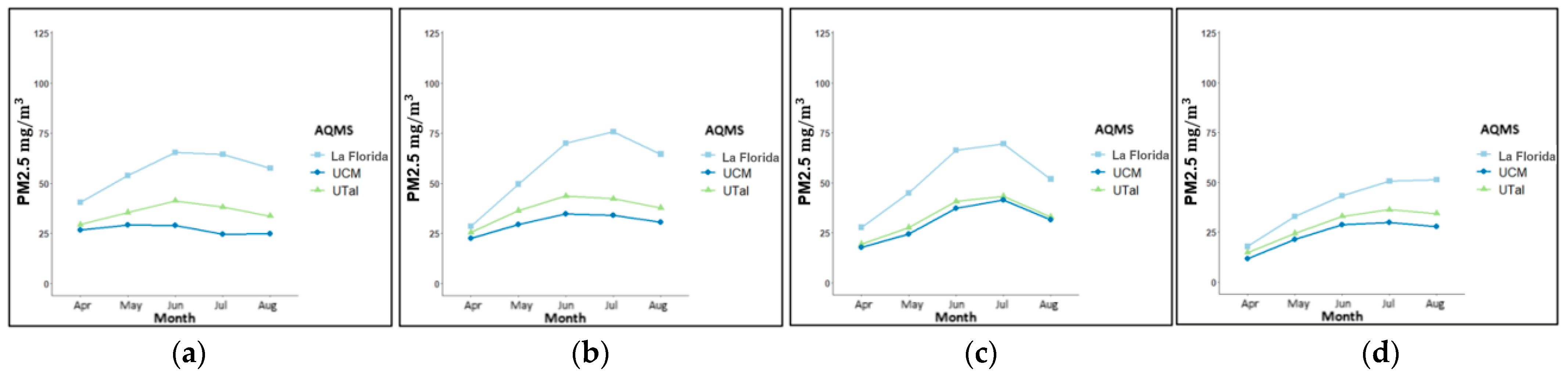
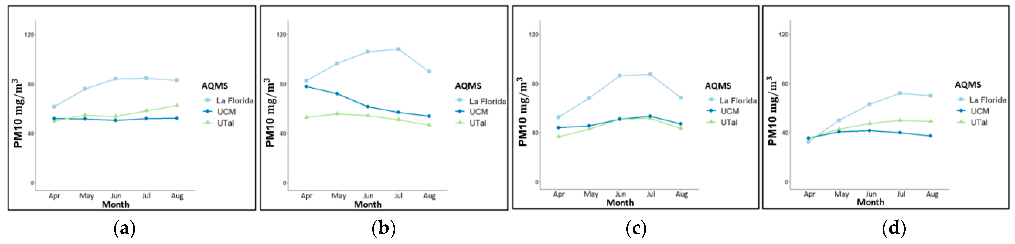
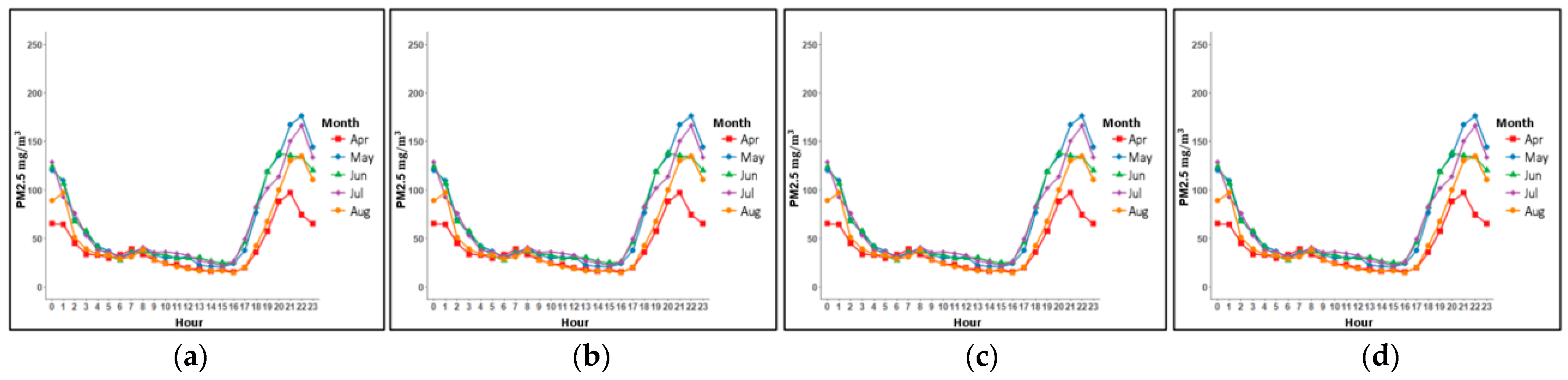
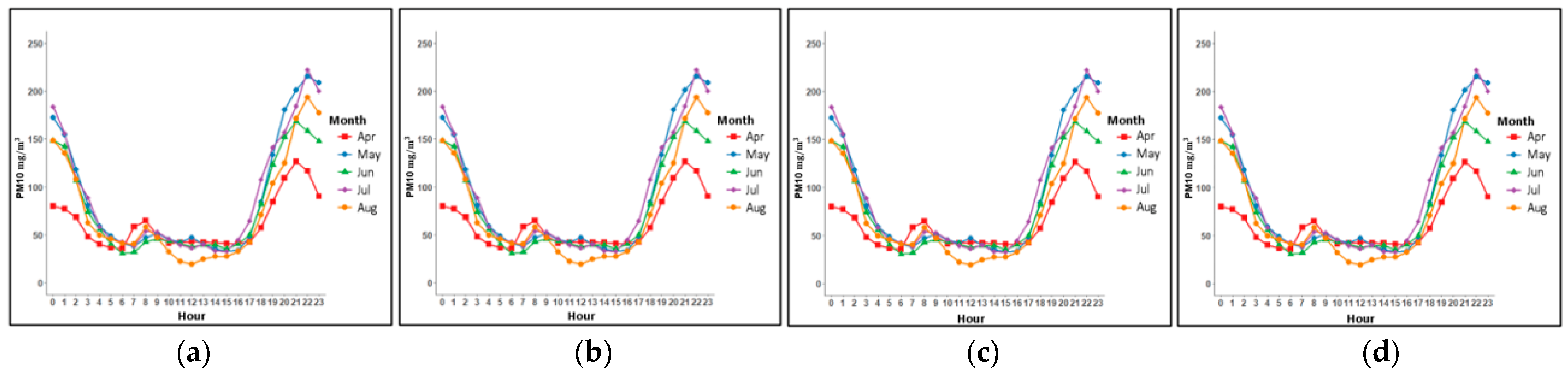
Hyperparameter optimization is to find, among all the models, those hyperparameters that return the best performance measure with the validation dataset. In this study, simple grid optimization was applied for hyperparameter optimization. The optimization parameters used were: C = 50, $\epsilon$ = 0.0075 and $\gamma$ = 1 × 10⁻⁵. These parameters were used for all models. The ML supervised classification algorithm SVR was used to predict PM levels. In detail, to evaluate the performance of the models used and establish improvements in their predictions, two new datasets were derived from the baseline and extended datasets with the same characteristics as the original datasets, but for the hourly range between 05:00 to 11:00 p.m. These new datasets were created due to the trends observed in Figure 6 and Figure 7, where an increase in PM concentrations was observed within this interval in the three AQMSs. Therefore, we carried out the training of 24 models to predict PM2.5 and PM10 levels in the three AQMSs of Talca city, considering the 24-h average and the average between 05:00 to 11:00 p.m. In this way, for each AQMS (UCM, UTAL and La Florida), eight models were implemented, for example, for UCM AQMS we have: UCM_baseline_PM2.5, UCM_baseline_PM10, UCM_extended_PM2.5, UCM_extended_PM10, UCM_baseline_PM2.5_5-11pm, UCM_baseline_PM10_5-11pm, UCM_extended_PM2.5_5-11pm and UCM_ extended _PM10_5-11pm.

Model Performance and Evaluation

The following tables show the results obtained during the training phase with data from 2014 to 2017 for La Florida AQMS, and from 2014 to 2016 for the UCM and UTAL AQMSs. For the evaluation of model performance, we use the determination coefficient R² and RMSE. For forecast accuracy evaluation, we use the MASE [18].

We separated the results for the training predictive models where the 24-h averages and the averages between 05:00 to 11:00 p.m. were used.

Table 5. R², RMSE and MASE for training models using 24-h average.

	PM10 Levels						PM2.5 Levels
AQMS	Baseline Dataset			Extended Dataset			Baseline Dataset			Extended Dataset
	R2	RMSE	MASE	R2	RMSE	MASE	R2	RMSE	MASE	R2	RMSE	MASE
La Florida	0.85	34.66	0.75	0.87	32.41	0.71	0.86	26.57	0.72	0.87	25.54	0.67
UCM	0.66	28.37	0.90	0.74	25.01	0.76	0.69	19.96	0.93	0.79	16.45	0.75
UTAL	0.81	22.33	0.65	0.85	20.40	0.59	0.84	15.82	0.65	0.88	13.59	0.56

and

Table 6. R², RMSE and MASE for training models using averages between 05:00 to 11:00 p.m.

	PM10 Levels						PM2.5 Levels
AQMS	Baseline Dataset			Extended Dataset			Baseline Dataset			Extended Dataset
	R2	RMSE	MASE	R2	RMSE	MASE	R2	RMSE	MASE	R2	RMSE	MASE
La Florida	0.87	45.95	0.52	0.88	42.76	0.48	0.87	36.70	0.50	0.87	35.76	0.47
UCM	0.67	37.87	0.63	0.75	33.41	0.55	0.71	27.30	0.61	0.81	21.76	0.52
UTAL	0.80	31.30	0.48	0.84	28.17	0.43	0.84	21.94	0.45	0.89	18.33	0.38

show the model performance results for the 24-h average and average between 05:00 to 11:00 p.m., respectively.

According to the results of Table 5, it is possible to note that, for each AQMS, the model performance, for the prediction of PM2.5 and PM10 concentrations, was improved for the extended datasets. In general, the determination coefficients obtained by the adjusted SVR models indicate a good fit in the 12 scenarios shown in Table 5. The R² were between 0.66 and 0.88, evidencing a good performance, especially in the adjusted models for the UTAL and La Florida AQMSs. Moreover, the RMSE values were smaller in models for the UCM and UTAL AQMS. In addition, the MASE values indicate that the forecast level of the models is good (MASE < 1), especially in the UTAL AQMS.

The training results shown in Table 6 indicate that for all AQMSs the performance of the model based on R² was between 0.67 and 0.88, which implies a good fit of the SVR model. Furthermore, as in the previous case, the RMSE values were smaller in models for the UCM and UTAL AQMS and better performance was observed for the extended database. When comparing the results of Table 5 and Table 6, we can observe that the R² were higher in the adjusted models for averages between 05:00 to 11:00 p.m. While the MASE values indicate a higher forecast level for the models for averages between 05:00 to 11:00 p.m. Subsequently, an external validation of the best models obtained in the training phase was made with year 2017 for the UCM and UTAL AQMS, and with year 2018 for the La Florida AQMS.

Table 7. R², RMSE and MASE for predictive models for 24-h average.

	PM10 Levels						PM2.5 Levels
AQMS	Baseline Dataset			Extended Dataset			Baseline Dataset			Extended Dataset
	R2	RMSE	MASE	R2	RMSE	MASE	R2	RMSE	MASE	R2	RMSE	MASE
La Florida	0.80	33.68	0.99	0.82	32.22	0.94	0.81	29.78	1.05	0.83	28.05	0.99
UCM	0.88	14.14	0.82	0.9	12.47	0.60	0.89	11.43	0.79	0.91	9.82	0.66
UTAL	0.91	11.80	0.91	0.9	12.48	0.67	0.92	9.75	0.61	0.90	11.37	0.75

and

Table 8. R², RMSE and MASE for predictive models for averages between 05:00 to 11:00 p.m.

	PM10 Levels						PM2.5 Levels
AQMS	Baseline Dataset			Extended Dataset			Baseline Dataset			Extended Dataset
	R2	RMSE	MASE	R2	RMSE	MASE	R2	RMSE	MASE	R2	RMSE	MASE
La Florida	0.85	41.02	0.57	0.85	40.37	0.56	0.86	33.69	0.56	0.87	32.18	0.55
UCM	0.93	15.43	0.52	0.93	14.44	0.44	0.94	11.86	0.42	0.94	12.04	0.44
UTAL	0.93	14.62	0.37	0.92	15.67	0.41	0.93	12.70	0.35	0.91	15.06	0.48

show the model´s performance for predicted PM10 and PM2.5 levels, based on statistics R², RMSE and MASE, for 24-h average data and average between 05:00 to 11:00 p.m., respectively.

According to the results of Table 7, the R² of the adjusted model for prediction of PM10 levels varied from 0.80 to 0.91 and from 0.81 to 0.92 for PM2.5 prediction. In Table 8, the R² of the adjusted model for PM10 prediction varied from 0.85 to 0.93 and from 0.86 to 0.94 for PM2.5 prediction. The RMSE values were smaller in models for the UCM and UTAL AQMS than in the training stage. In addition, according to Table 8, the MASE values indicates a higher forecast level in the models for averages between 05:00 to 11:00 p.m.

In general, the determination coefficients obtained by the adjusted SVR models indicate a good fit in the 24 scenarios shown in Table 7 and Table 8. However, the results obtained to predict PM10 and PM2.5 were better with the model for the extended dataset and averages between 05:00 to 11:00 p.m.

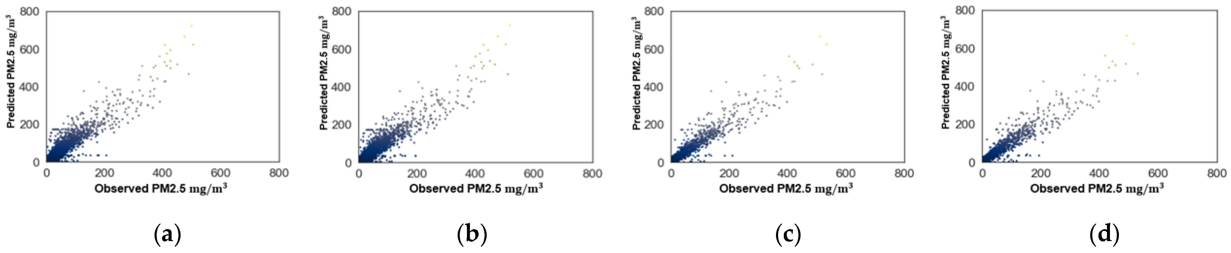
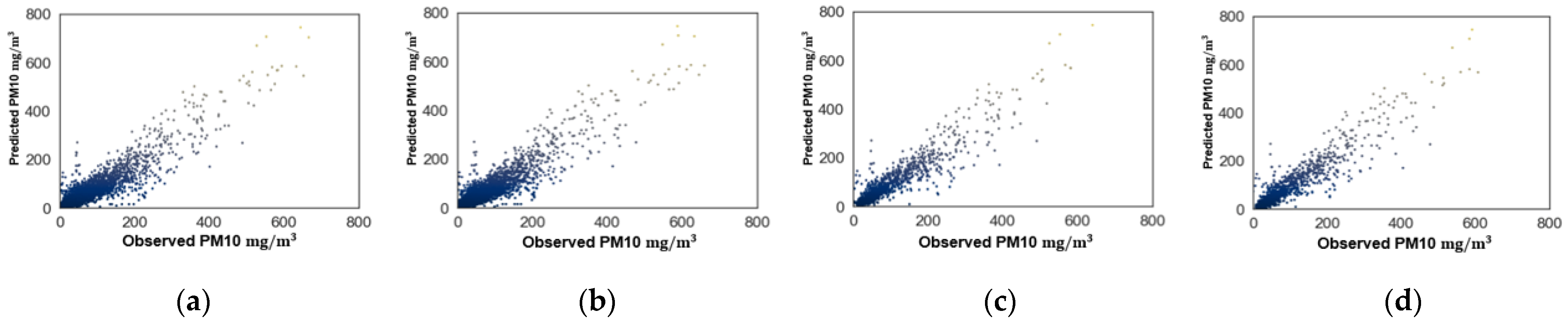
Finally, plots of the predicted versus observed PM10 and PM2.5 levels are shown in Figure 8 and Figure 9 for La Florida AQMS, respectively. Plots for the other AQMSs show similar behavior and are omitted here. In Figure 8 and Figure 9, predictively, the SVR model followed the trend of the observed data. However, a better level of prediction was observed in the plots for the extended dataset using the averages between 05:00 to 11:00 p.m. These predictions are shown in Figure 8 and Figure 9c,d.

Table 9. Chilean primary quality guidelines for PM concentrations in 24-h [4].

Condition	PM2.5 Concentration	PM10 Concentration
good	[0,49]	[0,149]
regular	[50,79]	[150,194]
alert	[80,109]	[195,239]
pre-emergency	[110,169]	[240,329]
emergency	≥170	≥330

shows the Chilean primary quality guidelines for PM2.5 and PM10 levels in 24-h. Next, the prediction capacity of the proposed models with respect to the primary quality guidelines for PM2.5 and PM10 were analyzed, based on which the degree of precision to detect critical episodes was determined.

Table 10. Categorization of observed and predicted PM2.5 concentrations based on Chilean primary quality guidelines in CEM period for extended dataset and averages between 05:00 to 11:00 p.m.

Condition
AQMS	Good		Regular		Alert		Pre-Emergency		Emergency
	Observed	Predicted	Observed	Predicted	Observed	Predicted	Observed	Predicted	Observed	Predicted
La Florida	64	61	26	19	21	9	25	20	17	11
UCM	115	109	19	13	8	6	8	8	3	3
UTAL	96	86	30	22	15	10	11	9	1	1

and

Table 11. Categorization of observed and predicted PM10 concentrations based on Chilean primary quality guidelines in CEM period for extended dataset and averages between 05:00 to 11:00 p.m.

Condition
AQMS	Good		Regular		Alert		Pre-Emergency		Emergency
	Observed	Predicted	Observed	Predicted	Observed	Predicted	Observed	Predicted	Observed	Predicted
La Florida	50	40	23	17	23	15	28	23	29	25
UCM	81	77	39	25	15	7	12	7	6	5
UTAL	61	61	41	21	26	13	19	12	6	6

contain the categorization of the observed and predicted concentrations according to the primary air quality regulations for each category (i.e., good, regular, alert, pre-emergency and emergency) for averages between 05:00 to 11:00 p.m. and PM2.5 and PM10 levels. Note that, in Table 10 and Table 11, we categorize the observed and predicted levels according to the categories indicated in Table 9; for example, in the La Florida AQMS there were 64 concentrations of PM2.5 in good condition, of which 61 were correctly predicted. The objective of these tables is to evaluate the predictive capacity of the proposed models.

As can be seen, in Table 10 and Table 11, the predicted values have a high accuracy; if we observe the alert, pre-emergency and emergency conditions, the model developed achieved a high prediction accuracy for these classes, which represented a minority in the CEM period. This is of great relevance, since, for the lifting of citizen restrictions in a timely manner, it is crucial to efficiently predict these minority classes due to their relevance to alert and manage critical episodes during the months of April to August.

Table 12. Correctly classified PM2.5 concentrations based on Chilean primary quality guidelines in CEM period for extended dataset and averages between 05:00 to 11:00 p.m. for La Florida AQMS.

	Good		Regular		Alert		Pre-Emergency		Emergency		Total
Good	488	91.9%	30	5.6%	6	1.1%	6	1.1%	1	0.2%	531
Regular	61	37.9%	82	50.9%	17	10.6%	1	0.6%	0	0.0%	161
Alert	3	2.8%	48	45.3%	37	34.9%	17	16.0%	1	0.9%	106
Pre-emergency	1	0.7%	8	5.8%	36	26.3%	80	58.4%	12	8.8%	137
Emergency	1	0.7%	3	2.2%	5	3.7%	32	23.5%	95	69.9%	136
Total	554	51.7%	171	16.0%	101	9.4%	136	99.7%	109	10.2%	1071

,

Table 13. Correctly classified PM2.5 concentrations based on Chilean primary quality guidelines in CEM period for extended dataset and averages between 05:00 to 11:00 p.m. for UCM AQMS.

	Good		Regular		Alert		Pre-Emergency		Emergency		Total
Good	792	96.0%	33	4.0%	0	0.0%	0	0.0%	0	0.0%	825
Regular	21	18.1%	71	61.2%	22	19.0%	2	1.7%	0	0.0%	116
Alert	0	0.0%	15	27.8%	35	64.8%	4	7.4%	0	0.0%	54
Pre-emergency	0	0.0%	1	2.4%	5	12.2%	33	80.5%	2	4.9%	41
Emergency	0	0.0%	0	0.0%	0	0.0%	3	8.6%	32	91.4%	35
Total	813	75.9%	120	11.2%	62	5.8%	42	3.9%	34	3.2%	1071

,

Table 14. Correctly classified PM2.5 concentrations based on Chilean primary quality guidelines in CEM period for extended dataset and averages between 05:00 to 11:00 p.m. for UTAL AQMS.

	Good		Regular		Alert		Pre-Emergency		Emergency		Total
Good	649	89.4%	73	10.1%	3	0.4%	1	0.1%	0	0.0%	726
Regular	2	1.2%	111	68.9%	44	27.3%	4	2.5%	0	0.0%	161
Alert	0	0.0%	7	9.5%	41	55.4%	24	32.4%	2	2.7%	74
Pre-emergency	0	0.0%	0	0.0%	3	4.0%	61	81.3%	11	14.7%	75
Emergency	0	0.0%	0	0.0%	0	0.0%	0	0.0%	35	100.0%	35
Total	651	60.8%	191	17.8%	91	8.5%	90	8.4%	48	4.5%	1071

,

Table 15. Correctly classified PM10concentrations based on Chilean primary quality guidelines in CEM period for extended dataset and averages between 05:00 to 11:00 p.m. for La Florida AQMS.

	Good		Regular		Alert		Pre-Emergency		Emergency		Total
Good	789	94.7%	25	3.0%	15	1.8%	4	0.5%	0	0.0%	833
Regular	27	30.7%	43	48.9%	12	13.6%	5	5.7%	1	1.1%	88
Alert	4	6.9%	22	37.9%	22	37.9%	9	15.5%	1	1.7%	58
Pre-emergency	1	2.3%	2	4.5%	10	22.7%	23	52.3%	8	18.2%	44
Emergency	0	0.0%	0	0.0%	1	2.1%	11	22.9%	36	75.0%	48
Total	821	76.7%	92	8.6%	60	5.6%	52	4.9%	46	4.3%	1071

,

Table 16. Correctly classified PM10 concentrations based on Chilean primary quality guidelines in CEM period for extended dataset and averages between 05:00 to 11:00 p.m. for UCM AQMS.

	Good		Regular		Alert		Pre-Emergency		Emergency		Total
Good	997	99.4%	6	0.6%	0	0.0%	0	0.0%	0	0.0%	1003
Regular	8	25.8%	16	51.6%	7	22.6%	0	0.0%	0	0.0%	31
Alert	1	5.3%	1	5.3%	14	73.7%	3	15.8%	0	0.0%	19
Pre-emergency	0	0.0%	0	0.0%	2	20.0%	7	70.0%	1	10.0%	10
Emergency	0	0.0%	0	0.0%	0	0.0%	0	0.0%	8	100.0%	8
Total	1006	93.9%	23	2.1%	23	2.1%	10	0.9%	9	0.8%	1071

and

Table 17. Correctly classified PM10 concentrations based on Chilean primary quality guidelines in CEM period for extended dataset and averages between 05:00 to 11:00 p.m. for UTAL AQMS.

	Good		Regular		Alert		Pre-Emergency		Emergency		Total
Good	964	99.7%	3	0.3%	0	0.0%	0	0.0%	0	0.0%	967
Regular	22	40.0%	31	56.4%	2	3.6%	0	0.0%	0	0.0%	55
Alert	1	3.7%	11	40.7%	12	44.4%	3	11.1%	0	0.0%	27
Pre-emergency	0	0.0%	0	0.0%	6	40.0%	9	60.0%	0	0.0%	15
Emergency	0	0.0%	0	0.0%	0	0.0%	3	42.9%	4	57.1%	7
Total	987	92.2%	45	4.2%	20	1.9%	15	114.0%	4	0.4%	1071

show the data correctly classified for each of the air quality categories (Table 9) and those that were misclassified in other categories. For each table, we also provide the respective percentages of correct classification. In detail, the contingency Table 12, Table 13 and Table 14 show the predicted air quality categories for PM2.5 levels in the case of La Florida, UCM and UTAL AQMSs. Meanwhile contingency Table 15, Table 16 and Table 17 show the predicted categories for PM10 levels for each AQMS.

In Table 12, Table 13 and Table 14, it is possible to observe that our models are capable of predicting PM2.5 levels for each category with high precision. In the case of La Florida AQMS, the prediction of each category was: good equals to 91.9%, regular equals to 50.9%, alert equals to 34.9%, pre-emergency equals to 58.4% and emergency equals to 69.9%. For UCM AQMS, prediction values were as follow: good equals to 96.0%, regular equals to 61.2%, alert equals to 64.8%, pre-emergency equals to 80.5% and emergency equals to 91.4%. Finally, in the case of UTAL AQMS, our model gave prediction values for each category as follows: good equals to 89.4%, regular equals to 68.9%, alert equals to 55.4%, pre-emergency equals to 81.3% and emergency equals to 100%. Specifically, we note that the prediction is good in the minority categories (i.e., alert, pre-emergency and emergency). These categories are very important due their relevance in the monitoring of critical episodes.

For PM10 prediction, Table 15, Table 16 and Table 17 show the values and percentage of successes for each category. In the case of La Florida AQMS, the prediction of each category was: good equals to 94.7%, regular equals to 48.9%, alert equals to 37.9%, pre-emergency equals to 52.3% and emergency equals to 75%. For UCM AQMS, prediction values were as follows: good equals to 99.4%, regular equals to 51.6%, alert equals to 73.7%, pre-emergency equals to 70% and emergency equals to 100%. Finally, in the case of UTAL AQMS, our model gave prediction values for each category as follows: good equals to 99.7%, regular equals to 56.4%, alert equals to 44.4%, pre-emergency equals to 60% and emergency equals to 57.1%.

4. Discussion

Based on the results obtained with the training dataset for all stations, it was observed that the best performance was obtained with the models that used the extended datasets, but limited to the hourly range from 05:00 to 11:00 p.m., both for PM10 and PM2.5 levels, as can be seen in Table 5 and Table 6. In the validation stage, it can be observed that the behavior of the models showed a similar trend, obtaining better results with the extended datasets within the limited hourly range for the PM10 and PM2.5 levels; see Table 7 and Table 8.

Regarding related studies in Talca city, only one was found in our literature search; this study was carried out in 2019 with the objective of predicting PM2.5 concentrations using deep neural networks [10]. In this study, the determination coefficients obtained were 0.65, 0.74 and 0.74 for La Florida, UCM and UTAL AQMS, respectively. Comparatively, the determination coefficients obtained in this study using the SVR model were 0.87, 0.94 and 0.91 for La Florida, UCM and UTAL AQMS, demonstrating better performance with respect to models based on neural networks. In addition, in our study, we implemented models to predict PM10 levels in order to provide a robust tool for decision-making since the primary Chilean air quality regulations require monitoring of PM2.5 and PM10 to inform decisions about critical air pollution episodes.

The main advantage of this research is the low computational consumption in the generation of predictive models based on SVR, once the hyperparameters have been optimized. With these models it was possible to obtain predictions with high accuracy, as observed in Table 7 and Table 8, better than the results obtained in similar investigations, for example those that have used multilayer neural networks for prediction.

Furthermore, Zeng et al. [11] used GAM to predict PM2.5 concentrations, based on multiple meteorological variables, in Chengdu, China. One of the GAMs developed in this study exhibited an adjusted coefficient of determination of 0.73, which is comparatively lower than the behavior shown with the models proposed by us.

Finally, the SVR-based model presented in this paper obtained comparatively superior results to the models described in the literature, highlighting the great potential of this tool for the classification of minority conditions, such as alert, pre-emergency and emergency. Moreover, it exceeded the estimates obtained by models based on neural networks, such as long short-term memory (LSTM) and statistical models, such as GAM (see [10,11]). The excellent performance of SVR makes it a viable and efficient alternative for the development of predictive models that help manage episodes of environmental emergency.

5. Conclusions and Future Investigation

In this study, predictive models based on machine learning techniques were implemented considering climatic and meteorological data, together with particulate matter levels to predict PM2.5 and PM10 in the three air quality monitoring stations in Talca, Chile. A total of 24 scenarios were considered in which the datasets were composed of baseline dataset, extended dataset, 24-h average data, and average between 05:00 to 11:00 p.m. Of these scenarios, 12 were used to predict PM10 and the others to predict PM2.5 levels.

Our models implemented with support vector regression indicate the capability to predict, with a high percentage of successes, not only the majority category (good and regular), but also the minority categories presented in the datasets, which corresponded to alert, pre-emergency and emergency. In this way, our methodology allows prediction, with high effectiveness, of critical episodes of air quality, for specific PM2.5 and PM10 levels.

Note that the proposed models are based on the real state of the environment of Talca city, such as the number and distribution of monitoring stations in time and space, real concentrations of particulate matter, and meteorological variables. If any of these conditions change, the proposed models must be adapted according to these changes.

Future research, arising from the present applied investigation, is proposed as follows: (1) development of an interface based on Python, where the proposed machine learning models are implemented with automatic daily data extraction from the National Air Quality Information System website, allowing the prediction of critical pollution episodes in real time for Talca city and for other cities in the country that have updated air quality monitoring data, (2) application of other machine learning techniques, such as long short-term memory neural networks for the prediction of PM concentrations in Talca city.

References

1. Scapini, V.; Carrasco, C.; Vergara Silva, C. Efectos de la contaminación del aire en atenciones de urgencia de la Región Metropolitana. Rev. Ing. Sist. 2018, 32, 55–73. [Google Scholar]
2. Ou, C.; Hedley, A.; Chung, R.; Thach, T.; Chau, Y.; Chan, K.; Yang, L.; Ho, S.; Wong, C.-M.; Lam, T. Socioeconomic disparities in air pollution-associated mortality. Environ. Res. 2008, 107, 237–244. [Google Scholar] [CrossRef] [PubMed]
3. Marchant, C.; Leiva, V.; Christakos, G.; Cavieres, M.F. Monitoring urban environmental pollution by bivariate control charts: New methodology and case study in Santiago, Chile. Environmetrics 2019, 30, e2551. [Google Scholar] [CrossRef]
4. MMA. Air Quality. Chapter 14 State of the Environment Report; National Environmental Information System, Ministry of the Environment of the Chilean Government: Santiago, Chile, 2021.
5. Cavieres, M.F.; Leiva, V.; Marchant, C.; Rojas, F. A methodology for data-driven decision making in the monitoring of particulate matter environmental contamination in Santiago of Chile. Rev. Environ. Contam. Toxicol. 2020, 250, 45–67. [Google Scholar] [CrossRef] [PubMed]
6. WHO. Particulate Matter. In Air Quality Guidelines for Europe; World Health Organization, Regional Office for Europe: Copenhagen, Denmark, 2000; Chapter 7.3. [Google Scholar]
7. Yáñez, M.; Baettig, R.; Cornejo, J.; Zamudio, F.; Guajardo, J.; Fica, R. Urban airborne matter in central and southern Chile: Effects of meteorological conditions on fine and coarse particulate matter. Atmos. Environ. 2017, 161, 221–234. [Google Scholar] [CrossRef]
8. MMA. Establishes Atmospheric Decontamination Plan for the Communes of Talca and Maule; Technical Report Decree 509; Ministry of Environment of the Chilean Government: Santiago, Chile, 2013.
9. Puentes, R.; Marchant, C.; Leiva, V.; Figueroa-Zúñiga, J.I.; Ruggeri, F. Predicting PM2.5 and PM10 Levels during Critical Episodes Management in Santiago, Chile, with a Bivariate Birnbaum-Saunders Log-Linear Model. Mathematics 2021, 9, 645. [Google Scholar] [CrossRef]
10. Astudillo, C.A.; González-Martínez, L.; Zapata-González, E. Predicting air quality using deep learning in Talca City, Chile. In Proceedings of the 10th International Conference on Pattern Recognition Systems, Tours, France, 8–10 July 2019. [Google Scholar]
11. Zeng, Y.; Jaffe, D.A.; Qiao, X.; Miao, Y.; Tang, Y. Prediction of potentially high PM2.5 concentrations in Chengdu, China. Aerosol Air Qual. Res. 2020, 20, 956–965. [Google Scholar] [CrossRef] [Green Version]
12. Awad, M.; Khanna, R. Support vector regression. In Efficient Learning Machines; Apress: Berkeley, CA, USA, 2015; pp. 67–80. Available online: https://link.springer.com/chapter/10.1007/978-1-4302-5990-9_4 (accessed on 23 April 2021).
13. Salini Calderon, G.A. Particulate Matter Analysis from Mid-sized Cities in the South of Chile. INGE CUC 2014, 10, 97–108. Available online: http://hdl.handle.net/11323/2610 (accessed on 14 March 2021).
14. Altman, N.S. An introduction to kernel and nearest-neighbor nonparametric regression. Am. Stat. 1992, 46, 175–185. [Google Scholar]
15. Palacios, C.A.; Reyes-Suarez, J.A.; Bearzotti, L.A.; Leiva, V.; Marchant, C. Knowledge Discovery for Higher Education Student Retention Based on Data Mining: Machine Learning Algorithms and Case Study in Chile. Entropy 2021, 23, 485. [Google Scholar] [CrossRef]
16. Vapnik, V. The Nature of Statistical Learning Theory; Springer Science & Business Media: Berlin/Heidelberg, Germany, 2013. [Google Scholar]
17. R Core Team. R: A Language and Environment for Statistical Computing; R Foundation for Statistical Computing: Vienna, Austria, 2021. [Google Scholar]
18. Hyndman, R.; Koehler, A. Another look at measures of forecast accuracy. Int. J. Forecast. 2006, 22, 679–688. [Google Scholar] [CrossRef] [Green Version]
Figure 1. Step-by-step description of the proposed methodology for the prediction of PM2.5 and PM10 levels.
Mathematics 10 00373 g001
Figure 2. Map of Talca city with its respective AQMSs, source Google Maps (https://www.google.cl/maps, accessed on 25 April 2021).
Mathematics 10 00373 g002
Figure 3. Correlogram for LF_PM10_extended where F1 to F24 are defined in Table 2 and Table 3.
Mathematics 10 00373 g003
Figure 4. Average PM2.5 levels by AQMS and month, during the CEM period in Talca, Chile for the years 2014 (a), 2015 (b), 2016 (c) and 2017 (d).
Mathematics 10 00373 g004
Figure 5. Average PM10 levels by AQMS and month, during the CEM period in Talca, Chile for the years 2014 (a), 2015 (b), 2016 (c) and 2017 (d).
Mathematics 10 00373 g005
Figure 6. Average PM2.5 levels per month and hour during the CEM period in AQMS La Florida for the years 2014 (a), 2015 (b), 2016 (c) and 2017 (d).
Mathematics 10 00373 g006
Figure 7. Average PM10 levels per month and hour during the CEM period in AQMS La Florida for the years 2014 (a), 2015 (b), 2016 (c) and 2017 (d).
Mathematics 10 00373 g007
Figure 8. Predicted versus observed PM2.5 levels for La Florida AQMS with (a) baseline data set for 24-h average, (b) extended dataset for 24-h average, (c) baseline dataset for averages between 05:00 to 11:00 p.m. and (d) extended dataset for averages between 05:00 to 11:00 p.m.
Mathematics 10 00373 g008
Figure 9. Predicted versus observed PM10 levels for La Florida AQMS with (a) baseline data set for 24-h average, (b) extended dataset for 24-h average, (c) baseline dataset for averages between 05:00 to 11:00 p.m. and (d) extended dataset for averages between 05:00 to 11:00 p.m.
Mathematics 10 00373 g009