Abstract
The development of shipping companies relies on multiple financing channels and requires decisions to be made regarding fleet management. Therefore, a firm’s performance should be modeled based on multiple decision variables. The purpose of this paper is to develop a quantitative approach for determining the investment portfolio of a shipping company taking into account the equity value. The proposed model rests on the mathematical programming. The objective is to maximize the cumulative free cash flow to equity, associated with the implementation of a long-term fleet replenishment program. The distinctive feature of the approach is that different cost of debt financing options and different levels of starting capital are considered. The enterprise can then be determined based on the optimal value of free cash flows to equity for each ratio of starting capital and the number of acquired vessels.
1. Introduction
Investments and financing thereof are key questions that require proper decisions to be made in every enterprise. The shipping industry is particularly versatile and, therefore, requires tailored decision models to find optimal solutions for business development. These issues have been discussed in the earlier literature to a certain extent. Benstock and Vergottis [1] looked into market cycles in shipping and their impact on investment decisions of shipping companies have been investigated. The high degree of uncertainty and risk in the shipping business makes it important to forecast and optimize cash flows. Harwood [2] discussed debt financing related to investment in the shipping industry, including credit and leasing schemes. Orfanidis [3] suggested an approach to shipping finance along with example of the Hellenic market. The role and features of debt financing for the shipping industry have been covered.
Stopford [4] examined the formation cash flows in shipping industry and financing investments in the purchase of vessels. Grammenos [5] discussed the economics and maritime nexus, with focus on shipping investment and finance. Tsai [6] addressed the problematique of equity valuation of shipping companies. Damodaran [7] considered different tools and techniques for investment valuation and determining the value of business, as well as problems of the formation of an investment portfolio. Schinas et al. [8] offered a theoretical analysis and practical insights into investment financing in the shipping industry. Financial management issues and reporting were discussed by Zhao et al. [9] and Zheng et al. [10].
Lapkina and Prykhno [11] presented an application of multi-project management approach in the shipping companies. Alexandridis et al. [12] emphasized that access to credit can determine the competitiveness of a capital-intensive business as well as its success or failure under adverse market conditions. Kidwell [13] addressed the problem of debt financing in shipping industry are investigated. Shipbuilding credits, bond loans and collaterals for loans in shipping industry were discussed.
The use of mathematical programming in investment and financial management has become more important with the increasing complexity of business decisions. Oliinyk [14] focused on creating an investment portfolio by a financial institution is considered. Onyshchenko at al. (2019) proposed an approach to determining the optimal road map for enterprise development. The optimization of the structure and parameters of the development road map was carried out based on the strategic network, which made it possible to form alternative variants of the road map. This network is based on the principle of the formation of transport networks [15].
Danyliuk et al. [16] focused on functional and investment strategies of technical development of enterprises. Kotenko et al. [17] developed mathematical methods for detection factors influencing the competitiveness of water transport.
Lapkina et al. [18] discussed the mathematical model for multiproject development of the shipping company. The optimization model of the maintenance of projects taking into account specificity of activity, resources and possibilities of the company was developed. Malaksiano [19] addressed the development of effective strategy for fleet renewal. Zhykharieva et al. [20] systematized the practical experience of state protectionism in the shipping industry, which affects investment activity and the formation of cash flows of shipping companies.
Nguyen [21] further clarified the characteristics of marine culture in the Northeast of Vietnam. Nitsenko et al. [22] showed that the risk of multimodal transportation in the ports of the Azov and Black seas can fluctuate substantially. Kurznack et al. [23] developed a model of long-term value creation that supports companies in creating long-term value and setting their strategies accordingly. Powell [24] considered approaches to business valuation modeling, clarifies assessment of enterprise value, terminal value, etc. Sagliaschi [25] discussed the way in which leverage and its expected dynamics impact on firm valuation is very different from what is assumed by the traditional static capital structure framework. The research characterized the firm’s valuation process within a dynamical capital structure environment, which affects the formation of investment portfolio.
Stamos and Zimmerer [26] considered the asset allocation strategies that aim at actively managing the volatility of multi-asset-class portfolios in response to time-varying volatility forecasts. They concluded that active volatility management is beneficial for most of the asset classes and for mixed asset portfolios. Tapia Campos [27] referred to problems and mechanisms of insurance in the international shipping, without which an effective investment in fleet is impossible.
Even though different optimization models have been proposed in the literature to streamline investment decisions in shipping companies, certain gaps still persist. Specifically, most of the existing quantitative models do not use time-dependent (dynamic) parameters to optimize the cash flows. The dynamic parameters allow taking into account different options for financing investments in fleet under different conditions and time of their realization. Accordingly, there is a need to further develop optimization models for investment analysis and business valuation based on the consolidated planning of the fleet.
This article aims to develop an optimization model for maximizing the equity value of a shipping company by picking the optimal options for the fleet management. The mathematical programming problem is developed to solve this issue. The proposed quantitative model involves behavioral assumptions and market-wide and company-specific parameters. An illustrative example is also provided.
The proposed approach allows maximizing accumulated free cash flows to equity of a long-term fleet replenishment program taking into account the time value of money in assessing the efficiency of investments. It is noteworthy that the proposed model is able to account for the dependence of control parameters on time. Thus, one is able to optimize free cash flows to equity not only with regard to the number of vessels and the share of debt financing, but also with regard to the time of their acquisition. Thus, the proposed optimization model allows behavioral assumptions and real-life market conditions to be combined to devise effective investment plans for shipping companies.
2. Problem Setting
The problem is finding the optimal investment plans (that maximize equity value) for a shipping company. An investment plan includes decisions for the fleet management and the choice of financing channels. Fleet management comprises decisions on investment projects for the new commissions and/or acquisition of second-hand vessels. The schedule for disposing of old vessels is developed based on their age and suitability for further operation. A company will purchase additional tonnage using a loan and/or financial leasing of vessels within a specified time interval. All indicators are calculated at the end of each period.
The accumulated discounted free cash flow to equity (FCFE) dependent on the of the fleet management decisions is used as the objective function. To develop the model, it is necessary to determine the structure of the cash flows over time. Moreover, both costs and revenues in the model must be linked to external conditions and operational parameters. Data on costs and revenues, included in calculations, may be constant or variable, discrete or continuous, depending on specific conditions.
The decision variables are (i) the numbers of vessels of each type that are acquired under loan and financial leasing agreements and (ii) the loan to value ratio and ratio that takes into account the share of leasing financing for the acquisition of vessels, which are used to impose restrictions on fleet management. The second group of variables is ratios that take into account the share of debt financing. If necessary, they can be converted into constants. It may be helpful to consider the share of debt financing offered by banks and/or leasing companies when assessing the financing options. If there is an interval in which the ratio of loan to value and the share of leasing financing may vary, the corresponding parameters can be specified in the model.
A necessary condition for implementation of the fleet replenishment program is the positive the balance of accumulated free cash flows to equity at any time. The negative value of the balance indicates the need to attract additional equity or debt finance. Thus, these cash flows are to be involved in the underlying calculations.
The model should allow for the parameters to vary over time. This renders free cash flow optimization not only taking into account the number of vessels and the share of debt financing, but also the time of their acquisition. It should be noted that the objective function of the model differs from net present value (NPV) for an individual investment project, as the calculations include cash flows from the operation of vessels, which the company owned at the beginning of the program.
The model uses the following restrictions. The total number of vessels of each type purchased during the entire period of investment program must not exceed the preset upper limit on the number of vessels of each type purchased by the company for the entire planning period. The total number of leasing vessels of each type for the entire period of investment program must not exceed the established upper limit of the number of leasing vessels of each type for the entire planning period.
The loans to finance the purchase of each type of vessel in each planning period, provided full repayment of the loans by the end of the fleet replenishment program, should be from 50 to 80% of the vessel market value. That is, the loan-to-value (LTV) should range from 0.5 to 0.8. For the remaining planning periods, provided that it is impossible to fully repay the loan by the end of the fleet replenishment program, new loan agreements are not concluded, i.e., LTV should be zero.
The amount of leasing financing for purchase of each type of vessel in each planning period, provided full lease repayments by the end of the fleet replenishment program, should be from 70 to 80% of the vessel market value. This implies the share of leasing financing from 0.7 to 0.8. In other planning periods, provided that it is impossible to fully repay lease payments by the end of the fleet replenishment program, new leasing agreements are not concluded, i.e., the share of leasing financing should be zero.
At the beginning of the first planning period (or at the end of the zero planning period) the amount of equity for loan and leasing transactions should not exceed the amount of cash starting capital of the company at the beginning of the investment program. At the beginning of each subsequent planning period, the amount of equity for loan and leasing transactions should not exceed the amount of the accumulated balance of FCFE. The balance of the accumulated FCFE in each subsequent year is not less than in the previous year. The accumulated FCFE at the end of each year, starting from the first year, should not be negative.
The book value of old, purchased and leased vessels of each type at the end of each planning period, starting from the first year, is determined taking into account depreciation for that period. The number of purchased and leased vessels of each type in operation in each planning period takes into account acquired vessels. The number of old vessels of each type in each planning period takes into account retired vessels.
The number of purchased and leased vessels of each type in each planning period should not be negative. Loan agreements are not concluded in periods when the debt cannot be repaid in full by the end of the fleet replenishment program. Leasing agreements are not concluded in periods when the lease payments cannot be repaid in full by the end of the fleet replenishment program. The number of old, purchased and leased vessels must be an integer. The starting cash capital of the shipping company should not be negative. It is assumed that the company does not invest in the fleet development program additional equity in subsequent years.
3. Methodological Approach
The investment portfolio for fleet development is a set of investment projects of a shipping company. The portfolio is established in accordance with the investment objectives of the investor and considered as an integral object of management. Taking into account the high value of vessels and long payback period, the main way of financing investments is debt financing. Here, various types of loans and financial leasing schemes play the main role.
The formation of the investment portfolio includes the selection of specific assets for investment, as well as the optimal distribution of invested capital across the acquired assets. These processes are based on the principles of investment management. The investment portfolio must be adequate to the capital being invested and meet the acceptable level of risk.
The investor needs to choose the most favorable time for investments and risk management methods that are adequate to the goals. Investors pursue the following goals when establishing the investment portfolio: maximizing the level of profitability, ensuring adequate capital growth, increasing enterprise value, achieving acceptable level of investment risks, maintaining liquidity of invested assets at acceptable level.
The aforementioned principles can be taken into account by embarking on the formation of the investment portfolio of a shipping company according to the following procedure:
- Stage 1.
- Identify the options for fleet acquisition projects. The number of candidate investment projects under consideration should exceed the number of projects to be actually implemented.
- Stage 2.
- Evaluation of the performance of individual investment projects.
- Stage 3.
- Short-listing of investment projects according to a system of requirements (e.g., compliance of investment projects with the strategy of a shipping company, investment volume and period, investment efficiency).
- Stage 4.
- In-depth examination of the short-listed investment projects based on indicators of return on investment, level of risk, liquidity.
- Stage 5.
- Final selections of projects in the portfolio taking into account the relationship between all the considered indicators based on maximizing profitability and investor’s attitude to level of risk.
The free cash flows to equity are maximized by varying the number of vessels of each type purchased over a period of time, and shares of debt financing. The model allows varying the financing investments methods for purchase of different types of vessels (equity, loans, financial leasing) under different conditions of their implementation and the level of starting capital. This allows for long-term investment planning. The value of money is also taken into account.
Intrinsic value (discounted cash flow, DCF) approach to enterprise valuation is based on determining the expected earnings, including proceeds from sale of assets. The two-stage DCF valuation model includes cash flows for the forecast period and the terminal value. The forecast period used in valuing a company is usually about five years. Using a forecast period of more than five years to determine the value of a company will call into question the accuracy of the estimate. Using terminal value to find the value of a company tries to solve problems that arise when the planning horizon is rather long. Earnings can be taken as the basis of calculation of different types of income, cash flows or dividends.
4. Mathematical Formulation
The model seeks to maximize the accumulated discounted free cash flows to equity from the implementation of the fleet replenishment program. The linear programming problem is set up. The following variables are used in the model: —number of type j vessels that are purchased, using equity or debt capital, in period t; —the number of type j vessels that are leased (with repayment by the end of the investment period) during period t; —loan to value ratio (LTV) for finance the purchase of type j vessel in period t (we set LTV to lie within 50–80% of the vessel market value as per common practice); —ratio that takes into account the share of leasing financing for acquisition of type j vessel in period t (for developed countries, it may be within 70–100% of the vessel market value, and 70–80% for the developing countries).
In addition, the following notations are used in the model:
- FCFE(t)—free cash flows to equity in period t;
- r—discount rate based on the weighted average cost of capital (WACC);
- T—number of time periods within investment program realization;
- —the upper limit of the number of type j vessels to be purchased for the entire planning period;
- —the upper limit of the number of type j leasing vessels for the entire planning period;
- —the number of types of old vessels, purchased vessels and leasing vessels;
- —the loan repayment period of type j vessels;
- —the period of the leasing agreement of type j vessels;
- I(t)—cash equity on the acquisition of all vessels in period t;
- H(t)—cash equity of the shipping company, which is invested in the program at the end of period t,
- H(0)—starting capital;
- F(t)—accumulated free cash flows to equity at the end of period t;
- —book value of type j old vessel, purchased vessel and leasing vessel in period t;
- —market value of type j purchased vessel in period t;
- —market value of type j leasing vessel in period t;
- —depreciation on old vessels, purchase vessels and leasing vessels of type j in period t;
- —total number of purchased vessels of type j in operation in period t;
- —total number of leasing vessels of type j in operation in period t;
- —the number of old vessels of type j in operating in period t;
- —the number of retired old vessels of type j in period t.
The linear programming problem for the fleet management and investment decisions takes the following form:
The objective function in (1) maximizes the accumulated discounted free cash flows to equity (FCFE) from the investment program for the entire planning period. The optimization of the accumulated discounted free cash flows to equity is subject to a number of constraints. The first two constraints in (1) restrict the total number of vessels by type to be acquired on credit and leasing, respectively, for the entire planning period.
The third and fourth constraints in (1) determine the loan to value ratio for the purchase of the type j vessels in period t. As new loan agreements are not concluded in period , the loan to value ratio and the loan value are zero. The fifth and sixth constraints in (1) determine the share of leasing financing for the purchase type j vessel in period t. As new leasing agreements are not concluded in period ,
the share of leasing financing in this period is zero, as well as the number of
type j vessels that are chartered on leasing terms.
The seventh and eighth constraints in (1) limit the amount of cash equity for purchase/financial leasing of all vessels. At the beginning of the first year (or at the end of zero year) the amount of cash equity under loan and financial leasing agreements should not exceed the amount of cash starting capital of the company at the beginning of the investment program. At the beginning of each subsequent year t, the amount of equity under loan and leasing agreements should not exceed the amount of the accumulated balance of free cash flows to equity.
The ninth constraint in (1) rules that the balance of accumulated free cash flows to equity in each subsequent year is not less than that in the previous year. Further on, the tenth and eleventh constraints govern the amount of accumulated free cash flows to equity. Additionally, the accumulated free cash flows to equity at the end of each year, starting from the first year, should not be negative. Constraints 12–17 determine the book value of type j old vessels, purchased vessels and leasing vessels in period t. Constraints 18–21 determine the number of vessels to be purchased and leasing vessels, respectively, in operation during period t. Constraints 22 and 23 determine the changes in the structure of fleet in operation, by vessel types, taking into account retired vessels in period t. The number of retired vessels is determined exogenously as per Constraint 24 in (1) taking into account the age and technical state of vessels.
Constraints 25 and 26 in (1) determine the number of vessels of each type to be purchased in period t taking into account that new loan agreements are not concluded in period . Constraints 27 and 28 stipulate the number of leasing vessels of each type in period t, and also take into account that new leasing agreements are not concluded in period . Constraint 29 indicates the value of the starting cash capital of the shipping company at the end of year 0. Constraint 30 determines that additional equity in the following years in the investment program is not invested, i.e.,.
To determine , we introduce the following notations:
- —cash flows from operations in period t;
- —capital expenditures in period t;
- —net debt issued in period t.
Free cash flows to equity are used to determine how much free cash will remain in the company after the payment of all its obligations [24]:
where the cash flow from operations obviously depends on the number of type j vessels that are purchased during period t, , using equity or debt capital, the number of vessels of type j that are leased during period t, , and interest of debt financing. Loan interest depends on the LTV ratio for financing the purchase of a type j vessel in period t, , and the ratio takes into account the share of leasing financing for the acquisition of a type j vessel in period t, .
Capital expenditures depend on the number of type j vessels, the LTV
ratio for financing the purchase of a type j vessel in period t, and ratio that takes into account the share of leasing financing for the acquisition
of a type j vessel in period t.
Net debt issued is the difference between new debt issued and debt repayments :
The net debt issued depends on the number of type j vessels that are purchased during period t, using equity or debt capital, the number of vessels of type j that are leased during period t, and interest of debt financing. Loan interest depends on the LTV ratio for financing the purchase of a type j vessel in period t and the ratio that takes into account the share of leasing financing for the acquisition of a type j vessel in period t.
To describe the operating cash flows, we use the following notations:
- —operating cash flows of old, purchased and leased vessels in period t, respectively;
- —annual operating revenue of old, purchased and leased type j vessels in period t, respectively;
- —annual operating expenditures of old, purchased and leased type j vessels in period t, respectively;
- —income tax from operating old, purchased and leased type j vessels in period t, respectively;
- —loan interest for type j vessels in period t;
- —leasing interest for type j vessels in period t;
- —market daily time charter equivalent for type j vessels in period t;
- —operational time budget for type j vessels in period t;
- —average daily operational expenditures of type j vessels in period t.
The operating cash flow for each period is given by:
The cash flow from operations of old, purchased and leased vessels in period t, respectively are obtained as:
The operating revenue and operating cost for old, purchased and leased vessels of type j in period t are calculated as follows:
When calculating the capital expenditure and net debt issued, the following notations are needed:
- —net value of sales of the old vessel of type j, retired in period t, which may be defined as the residual value or scrap value.
- —cash equity on the acquisition of type j vessels under leasing contract in period t;
- , —net debt issued due to purchase and leasing of type j vessels in period t, respectively;
- —loan for purchase of type j vessels in period t;
- —repayment of principal debt by all loan agreements for purchase of all type j vessels in period t;
- —repayment of the principal debt by loan agreement for purchase of type j vessels in period t, concluded in period (at the end of period ). Repayments are made from the period , and ended in period ;
- —loan for purchase of type j vessels, received in period , ;
- —balance of loan debt for purchase of type j vessels in period t;
- —own money for purchase of type j vessels in period t;
- —own money for purchase of vessels of all types in period t;
- —lease financing (for calculation of annual lease payment) for type j vessels in period t;
- —amount of lease financing for type j vessels under agreements, concluded in period , ;
- —coefficient taking into account reimbursement of the lessor’s expenses and commission under type j vessels agreement, concluded in period t;
- —total amount of leasing payment in year t under leasing agreement by type j vessels, concluded in period t;
- —total amount of leasing payment in year t under leasing agreement by type j vessels, concluded in period (at the end of period ). Payments are made from the period and ended in period ;
- —principal leasing payment under all leasing agreement for type j vessels in period t;
- —principal leasing payment under all leasing agreement for type j vessels in period (at the end of period ). Payments are made from the period and end up in period ;
- —own money for acquisition of type j vessels under financial leasing agreements in period t;
- —own money for acquisition of all types of vessels under financial leasing agreements in period t.
The capital expenditures are calculated taking into account sales of old vessels, purchase of new vessels and payments for leasing vessels in period :
The capital expenditures from sale of old vessels and takes into account the projected residual (resale) vale of purchased vessels at the end of the investment program implementation period is given by:
The net debt issued connected with financing of purchase and leasing of vessels in period t is defined as:
The net debt issued associated with borrowing for the acquisition of type j vessels in period t is calculated as follows:
The loan for the purchase of type j vessels in period t is given by:
The equity paid by the company under the loan agreement in period t for the purchase of type j vessels is given by:
The principal debt in year t under a loan agreement for the purchase of type j vessels, concluded during the period , is calculated in the following manner:
The repayment of the principal debt under all loan agreements for the acquisition of type j vessels in period t is defined as:
The equity required for the acquisition of ships of all types on the basis of loan in period t is calculated by:
The net debt due to financial leasing taking into account that vessel residual value at the end of leasing period is zero. Thus, the net debt issued due to leasing is calculated as:
The leasing financing (annual leasing payments) for all type j type vessels in period t is given by:
The initial payment, paid by the shipping company, for the acquisition of type j vessels under a financial leasing agreement in period t is defined as:
The leasing payment in year t under a leasing agreement for the acquisition of type j vessels, concluded in period , is calculated as follows:
The payments under all leasing agreements for the acquisition of all type j vessels in period t are obtained via:
The principal leasing payment in year t under a leasing agreement for the acquisition of type j vessels, concluded in period
The principal leasing payments under leasing agreements for the acquisition of all type j vessels in period t are defined as follows:
Own money (cash) required for the acquisition of vessels of all types under a leasing agreement in period t is calculated as:
Own money required for the acquisition of vessels of all types in period t is obtained as:
5. Results
An empirical example of a shipping company operating with two old dry cargo vessels of different types is considered to verify the proposed model. It is assumed that the vessel of type 1 is to be disposed of at the end of year 4 and the vessel of type 2 at the end of year 5. Then, buying new vessels of type 3 and type 4 using a loan and vessels of type 5 using financial leasing based on bareboat charter agreement are foreseen. Daily OPEX grows by 1% annually on old vessels and by 0.5% annually on new vessels. The loan interest is 5%, the rate of leasing interest—7%. The rate of income tax is 18%, the depreciation rate for balance method—15% per year. WACC is calculated for each option taking into account share and value of debt and equity. Equity value is 11%. For options with share of debt by loan and leasing agreements 80% the WACC is 6.7%.
Calculations are performed using the Microsoft Excel Solver. The results of the calculations described in Section 4 assuming the number of purchased vessels varying from 5 to 10 and starting capital ranging between 2 and 5 million USD are presented in Figure 1. Figure 1 shows the dependence of the accumulated discounted free cash flow on the number of vessels with different starting capital. It can be seen from the results that the value of the accumulated discounted free cash flow depends on the number of acquired vessels more than the amount of available starting capital.
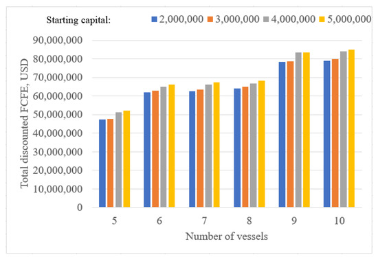
Figure 1.
Total discounted FCFE (in USD) across different numbers of purchased vessels and levels of starting capital.
The optimized discounted FCFE increases with the number of acquired vessels as an increase in the number of vessels in operation, subject to their profitable operation, makes it possible to increase the cash flows. The coefficients that take into account the share of debt financing for loan and financial leasing are close to the maximum value (80%), which is explained by the positive effect of financial leverage. At different intervals of change in the starting capital, changes in the optimal values of objective function with an increase in the number of vessels occur at different rates, which is associated with the ratio of the value of acquired vessels and accumulated cash flows in certain years (Table 1).

Table 1.
Differences in the total discounted FCFE for different numbers of the purchased vessels (as compared to the extreme case of five vessels) for each level of the starting capital.
The developed model makes it possible to take into account various financing schemes for the acquisition of vessels, vary loan interest rates and the cost of lease financing, and calculate options for different amounts of starting capital. As the initial data, various scenarios of changes in the level of freight rates, prices for vessels, operational expenditure can be used.
To determine an enterprise value (EV), we will use the following notations:
- FCFF (t)—free cash flows to the firm in period t;
- WACC—weighted average cost of capital;
- TV—the terminal value of business;
- Growth—constant rate of long-term growth of free cash flows.
An enterprise value can be determined by discounting the expected free cash flows to the firm (i.e., cash flows balance after all operating expenses, reinvestment and taxes, but before any payments by liabilities and shares) at the weighted average cost of capital [24]:
Free cash flows to the firm are generated by the business and do not include financial costs such as interest on debt financing. Reconciling free cash flows to equity and free cash flows to the company yields [24]:
The terminal value may be defined using the growing perpetuity method [24]:
The company value can be determined based on the optimal value of objective function for each ratio of the amount of starting capital and the number of acquired vessels:
For example, for the option with the limitation of the 8 acquired vessels and the starting capital USD 3 million, taking into account the optimal value of the objective function USD 64.923 million and the estimated terminal value of the company before discounting USD 223.792 million calculated with growth 1% per year, the enterprise value at the end of the 10th year, defined by the Formula (36), will be USD 294.221 million.
6. Discussion
A wide range of potential sources of financing for investment projects of shipping companies makes it necessary to select the most effective combination thereof. A number of objective and subjective factors influence the choice of a financing scheme and specific sources for the formation of investment capital of a shipping company. These include the organizational and legal form of a company, the size of the enterprise, availability of alternative sources of financing, the cost of capital raised from various sources, condition of the freight market and the phase of the shipping market cycle, the conjuncture of the financial market and corporate tax level.
In addition, the level of freight rates has an impact on the prices of ships, and, therefore, on the amount of investment. The choice of the right investment time significantly affects the investment result. The return on equity depends on the condition of the freight market. Investors, who chose the timing of the asset purchase that coincided with the low conjuncture of the freight market, received a higher return on investment, and vice versa. This is due to the fact that the value of assets in the year of purchase was much lower than in the subsequent period with the increase in market conditions and the sale of assets.
It should be noted that shipping companies, that transport goods in different segments of the freight market, do not have the opportunity to significantly reduce risks by diversifying the portfolio of investments in fleet development. The fundamental economic factors, which affect one segment of the freight market, usually affect other segments (changes in general economic conditions, industrial production, condition of financial market). For realizing the economic goals of investment shipping companies are usually aimed at obtaining a certain level of profitability and operate within an acceptable level of risk.
The modeling requires further research and should take into account the influence of exogenous market factors in the objective function. The two-step approach to discounted cash flows valuation may be a general solution to the problem taking into account uncertainty. For defining the terminal value of the business, it may be appropriate to use the methods of growing perpetuity and terminal exit value.
7. Conclusions
This paper presented a quantitative model for determining the decisions for a long-term fleet replenishment program. This is crucial for the formation of the investment portfolio of a shipping company. They key underlying assumption is maximization of the cumulative free cash flows to equity. The decision variables of the model include the number of vessels of certain types, acquired using equity financing/loan/financial leasing in a certain period alongside loan to value ratio and share of leasing financing. This allows for the decisions to be adjusted in regard to the conditions imposed by the creditors on the debt financing. The model involves the dynamics in the parameters, which is beneficial for long-term fleet replenishment programs. Thus, value of money is taken into account when assessing the performance of investments.
The model validation was carried out by considering the example of a shipping company operating dry cargo vessels. The results showed the dependence of the accumulated discounted free cash flow on the number of vessels and starting capital level. Non-monotonic relationships were found between the starting capital level and the discounted free cash flow to equity (considering the relative growth in the free cash flow in a case with the maximum number of vessels to a case with the minimum number of vessels across different levels of starting capital). This suggests that the use of the model is beneficial in unveiling the effects of choosing different investment strategies.
The enterprise value can be determined based on the optimal total value of free cash flows to equity for each level of the starting capital and the number of acquired vessels. The main advantage of using optimization models in investment planning is the simultaneous consideration of all the market conditions and behavioral assumptions. The developed approach can be used for other industries after adjusting the mathematical program.
Author Contributions
Conceptualization, V.Z. and V.N.; methodology, O.B., T.B. and O.V.; validation, O.V and T.B..; formal analysis, V.Z. and V.N.; investigation, V.Z.; resources, V.Z. and O.V.; writing—original draft preparation, O.B., V.Z. and D.S.; writing—review and editing, T.B., D.S. and V.N.; supervision, O.B. and V.Z.; project administration, O.B. and V.Z; funding acquisition, O.B. All authors have read and agreed to the published version of the manuscript.
Funding
This study was carried out as part of the project «Belt and Road Initiative Institute for Chinese-European studies» and was funded by the Guangdong University of Petrochemical Technology.
Institutional Review Board Statement
Not applicable.
Informed Consent Statement
Not applicable.
Data Availability Statement
The data are available from the corresponding author upon reasonable request.
Acknowledgments
Thanks to Guangdong University of Petrochemical Technology for supporting and donating this research. Thanks to Odesa National Maritime University for supporting this research.
Conflicts of Interest
The authors declare no conflict of interest.
References
- Benstock, M.; Vergottis, A. Econometric Modelling of World Shipping; Chapmen & Hall: London, UK, 1993. [Google Scholar]
- Harwood, S. Shipping Finance; Euromoney Books: London, UK, 1995. [Google Scholar]
- Orfanidis, A. Shipping Finance: Approach to the Hellenic Market; National Technical University of Athens: Athens, Greece, 2004. [Google Scholar]
- Stopford, M. Maritime Economics, 3rd ed.; Routledge: New York, UK, USA, 2009. [Google Scholar]
- Grammenos, C. The Handbook of Maritime Economics and Business; Informa Law from Routledge: London, UK, 2010. [Google Scholar]
- Tsai, T. Equity Valuation of Shipping Companies; Nanyang Technological University: Nanyang, Singapore, 2011. [Google Scholar] [CrossRef]
- Damodaran, A. Investment Valuation: Tools and Techniques for Determining the Value of Any Asset; John Wiley & Sons Inc.: New York, NY, USA, 2012. [Google Scholar]
- Schinas, O.; Grau, C.; Johns, M. HSBA Handbook on Ship Finance; Springer: Basel, Switzerland, 2014. [Google Scholar]
- Zhao, Y.L.; Liu, F.Y.; Liu, C.Y.; Usman, M.; Dutta, K.D. Readability of Annual Report and Inefficient Investment: Evidence from Debt Financing. Transform. Bus. Econ. 2020, 19, 166–190. [Google Scholar]
- Zheng, X.; Zhai, Y.; Wang, Z.; Song, J.; Wu, S. Firm Valuation Based on an Improved Ohlson Model. Transform. Bus. Econ. 2020, 19, 74–91. [Google Scholar]
- Lapkina, I.; Prykhno, Y. Multi-Project Management in Companies Development. PM World J. 2015, 4. Available online: https://pmworldlibrary.net/pmworld-journal-archives/ (accessed on 6 August 2021).
- Alexandridis, G.; Kavussanos, M.G.; Kim, C.Y.; Tsouknidis, D.A.; Visvikis, I.A. A survey of shipping finance research: Setting the future research agenda. Transp. Res. Logist. Transp. Rev. 2018, 115, 164–212. [Google Scholar] [CrossRef]
- Kidwell, J. Maritime Finance; Institute of Chartered Shipbrokers (ICS): London, UK, 2018. [Google Scholar]
- Oliinyk, V. Optimization of investment portfolio management. Serb. J. Manag. 2019, 14, 373–387. [Google Scholar] [CrossRef]
- Onyshchenko, S.; Bondar, A.; Andrievska, V.; Sudnyk, N.; Lohinov, O. Constructing and exploring the model to form the road map of enterprise development. East. Eur. J. Enterp. Technol. 2019, 5, 33–42. [Google Scholar] [CrossRef] [Green Version]
- Danyliuk, V.; Riepina, I.; Shafalyuk, O.; Kovylina, M.; Nitsenko, V. Functional and investment strategies of technical development of enterprises. Nauk. Visnyk Natsionalnoho Hirnychoho Universytetu 2020, 3, 115–121. [Google Scholar] [CrossRef]
- Kotenko, S.; Nitsenko, V.; Hanzhurenko, I.; Havrysh, V. The Mathematical Modeling Stages of Combining the Carriage of Goods for Indefinite, Fuzzy and Stochastic Parameters. Int. J. Integr. Eng. 2020, 12, 173–180. [Google Scholar] [CrossRef]
- Lapkina, I.; Prykhno, Y.; Lapkin, O. Content optimization of the development of multi-project of a shipping company. East. Eur. J. Enterp. Technol. 2020, 3, 50–57. [Google Scholar] [CrossRef]
- Malaksiano, M. Non-specialized vessel acquisition and operation projects, considering their suitability for oversized cargo transportation. Tend. Attual. Della Mod. Ric. Sci. 2020, 3, 79–83. [Google Scholar] [CrossRef]
- Zhykharieva, V.; Shyriaieva, L.; Vlasenko, O. Current trends of protectionism in shipping industry. Transp. Probl. 2019, 14, 89–100. [Google Scholar] [CrossRef] [Green Version]
- Nguyen, N.T. Marine Culture of Northeast Vietnam: Approaching from the Theory of Culture Ecology. Future Hum. Image 2020, 13, 66–75. [Google Scholar] [CrossRef]
- Nitsenko, V.; Kotenko, S.; Hanzhurenko, I.; Ingram, K.L. Determination of Weight Coefficients for Stochastic and Fuzzy Risks for Multimodal Transportation. J. Phys. Conf. Ser. 2020, 1529, 032007. [Google Scholar] [CrossRef]
- Kurznack, L.; Schoenmaker, D.; Schramade, W. A model of long-term value creation. J. Sustain. Financ. Invest. 2021, 1–19. [Google Scholar] [CrossRef]
- Powell, S. Business Valuation Modeling. Corporate Finance Institute. 2021. Available online: https://courses.corporatefinanceinstitute.com (accessed on 6 August 2021).
- Sagliaschi, U. Dynamical Corporate Finance: An Equilibrium Approach; Springer: Basel, Switzerland, 2021. [Google Scholar]
- Stamos, M.; Zimmerer, T. Managing portfolio volatility. J. Portf. Manag. Multi-Asset. 2021, 47, 99–109. [Google Scholar] [CrossRef]
- Campos, E.E.T. The Panama Canal and its False Security and Defense. Ukr. Policymaker 2021, 8, 117–120. [Google Scholar] [CrossRef]
Publisher’s Note: MDPI stays neutral with regard to jurisdictional claims in published maps and institutional affiliations. |
© 2022 by the authors. Licensee MDPI, Basel, Switzerland. This article is an open access article distributed under the terms and conditions of the Creative Commons Attribution (CC BY) license (https://creativecommons.org/licenses/by/4.0/).