Article

Optimal Power Flow Analysis Based on Hybrid Gradient-Based Optimizer with Moth–Flame Optimization Algorithm Considering Optimal Placement and Sizing of FACTS/Wind Power

1
Department of Electrical Engineering, Faculty of Engineering, Aswan University, Aswan 81542, Egypt
2
Electrical & Electronics Engineering Technology Department, Royal Commission Yanbu Colleges & Institutes, Yanbu Industrial City 46452, Saudi Arabia
*
Authors to whom correspondence should be addressed.
Mathematics 2022, 10(3), 361; https://doi.org/10.3390/math10030361
Submission received: 15 December 2021 / Revised: 15 January 2022 / Accepted: 21 January 2022 / Published: 25 January 2022
(This article belongs to the Special Issue Numerical Optimization and Applications)

Abstract

:
Optimal power flow (OPF) is one of the most significant electric power network control and management issues. Adding unreliable and intermittent renewable energy sources to the electrical grid increase and complicates the OPF issue, which calls for using modern optimization techniques to solve this issue. This work presents the optimal location and size of some FACTS devices in a hybrid power system containing stochastic wind and traditional thermal power plants considering OPF. The FACTS devices used are thyristor-controlled series compensator (TCSC), thyristor-controlled phase shifter (TCPS), and static var compensator (SVC). This optimal location and size of FACTS devices was determined by introducing a multi-objective function containing reserve costs for overestimation and penalty costs for underestimating intermittent renewable sources besides active power losses. The uncertainty in the wind power output is predicted using Weibull probability density functions. This multi-objective function is optimized using a hybrid technique, gradient-based optimizer (GBO), and moth–flame optimization algorithm (MFO).

1. Introduction

Electrical utilities always strive to find the best solutions for scheduling generation to lower the cost of production and satisfy safe and reliable operating restrictions and power transmission restrictions. Optimal Power Flow (OPF) is a non-linear, complicated optimization technique. The main objective of the OPF problem is to reach the best scheduling of control variables to decrease power losses and fuel cost, taking into account the achievement of the permissible limits in the system [1,2,3]. The OPF issue was developed utilizing a multi-objective function subject to set of constraints. The goal of OPF issue is to piecewise optimize a function with one or several objectives, such as gasoline cost, fuel cost reduction due to the valve-point impact, voltage profile enhancement, decrease of emissions, and stability of voltage, while taking limitations on equality and inequality into account. Controls variables in the OPF issue are transformer tap ratios, active or reactive power of generators, and bus voltages, whereas state variables are reactive power of the output generator and voltage of the load bus [4,5]. In optimization problems, different methods were created to solve OPF. Initially, a variety of mathematical methodologies were used, including interior point [6], linear programming [7], and Newton Raphson [8], to address the OPF problem. However, the results of these approaches were far from ideal, particularly for complex and large systems, and high-dimensional problems are tough to solve. These approaches have some drawbacks, such as a tendency to converge to local optimums and a lengthy computation time. Furthermore, because of their non-linear properties, these approaches are ineffective for issues involving valve-point effects. As a result, heuristic techniques have largely superseded traditional mathematical methods for solving electric power system issues. Heuristic methods for issue resolution can deliver more effective and fast answers when compared to traditional techniques. Heuristic approaches are frequently influenced by natural laws, biological characteristics, or observed collective behavior. Various heuristic methods have recently been developed, such as krill herd algorithm (KHA) [9], moth swarm algorithm (MSA) [10], grey wolf optimization with pattern search (GWO-PS) [11], salp swarm optimizer (SSO) [12], modified rao-2 algorithm [13], a joint self-adaptive particle swarm optimization (SPSO), and differential evolution algorithms [14], and employed in the OPF problem’s solution. In 2002 [15], the author employed the PSO to minimize overall cost, voltage enhancement, as well as voltage stability in IEEE 30-bus system. In 2003 [16], the author used the simulated annealing (SA) approach to reduce fuel costs in IEEE 30-bus systems. In 2004, the GA [17] was used to reduce the cost of gasoline in an IEEE 30-bus system. In 2012, the author used the GSA to minimize fuel cost, voltage profile improvement, and voltage stability in IEEE 30- and 57-bus systems. In 2015 [18], the author used the chaotic krill swarm algorithm (CKSA), while in 2017, different objectives were decreased, such as fuel cost, power loss, and emissions, using moth swarm algorithm (MSA) [10]. Fossil fuels utilized for the production of electricity in electric power networks have now reached the end of their useful life. Furthermore, hydrocarbons are to blame in order to reduce greenhouse gas emissions, which are created by CO2, NO2, and SO2, which contribute to global warming issues. A global majority has agreed to reduce emissions because of rising environmental consciousness and economic concerns [19]. Wind energy is a popular renewable energy source because it is long-lasting, ecologically benign, and cost-effective [20,21]. It has significant benefits in terms of lowering fuel costs and reducing pollutants. However, in this analysis, noise pollution and investment expenses were not taken into account. Wind power has now been included in the answer to the OPF problem by researchers. In 2015 [22], the authors solved the OPF challenge by employing the modified bacteria foraging algorithm (MBFA) to combine wind and fossil fuel generation units [20], while in 2016 [23], the author integrated wind units into an IEEE 14-bus system, and the OPF issues were handled using quadratic programming. Despite all of this development, the wind speed is unpredictably variable is a major issue. The weibull probability distribution function (PDF) is widely employed in long-term distribution problems for wind speed calculation [19]. In the operation of electric power systems, a lack of reactive power produces issues, such as voltage drop, variations in voltage, and voltage collapse, and voltage instability in severe circumstances. There are numerous options for dealing with the aforementioned situations; to mention a few, employing reactive power compensation and load shedding is used, which is less compatible than reactive power injection methods. Furthermore, generators and capacitor banks generate reactive power that is extremely sluggish to adjust to unexpected variations in load level. FACTS devices technology may be an appropriate option in this case. FACTS devices can help electric networks in a variety of ways, including lowering power losses, voltage stability enhancement, and improving the security of the network [24,25]. FACTS devices are extremely beneficial to a power grid; including them in OPF issues increases the difficulty of finding a good solution. To this purpose, the majority of methodologies in the papers to resolve the OPF issue using FACTS devices are based on heuristic and metaheuristic algorithms [26,27], with a quick overview of this set of algorithms given below: hybrid particle swarm optimization, particle swarm optimization (PSO) and adaptive GSA [28], krill herd algorithm (KHA) [29], fuzzy harmony search algorithm (FHSA) [30], bAT search algorithm [31], self-adaptive DE (SADE) [32], and symbiotic organisms search (SOS) algorithm [33]. Many attempts have been made in recent decades to identify effective techniques due to the significant nonlinearity of optimum power flow (OPF), and the inclusion of unpredictable and intermittent renewable sources into the electrical network increases the problem’s complexity; in this paper, the authors suggest machine learning (ML), improved salp swarm algorithm (ISSA), deep belief network (DBN), and combining chaotic particle swarm optimizer and gravitational search algorithm to solve the OPF problem [34,35,36,37], respectively. In practice, power plants face a number of practical limits, two of which include the valve-point impact and various fuels option; however, in order to arrive at a more realistic solution, certain constraints must be considered, and each is discussed further below [38]:
  • To begin, power plants can be powered by a number of fuels, including fossil, natural gas, and so on. As a result, it is possible to utilize various cost coefficients for different fuels.
  • In thermal power plants, a large number of valves are employed to regulate steam flow and unit output power. It is worth noting that opening the steam-admission valves can cause rapid variations in active power losses. In addition, it adds additional ripples to the cost function of generators as a result of the abrupt increase in active power losses.
However, we can summarize the main contribution of the paper as follows:
  • Presenting and employing a novel proposed meta-heuristic methodologies for a transmission system with unexpected wind power and FACTS devices.
  • Thermal power and wind power cost models are presented in this paper in detail.
  • The models of three facts devices (TCSC, TCPS, and SVC) are presented in this paper in detail.
  • This paper proposes a meta-heuristic optimization technique known as hybrid gradient-based optimizer and moth-flame optimization algorithm (GBO-MFO) technique to minimize the generation cost, reduce the power losses, minimize the cost and power losses, and compare with three other techniques (GBO, MFO, SMA, and CFA).
  • Four cases are studied in this paper with the following aims: minimizing the generation cost, reducing the power losses, minimizing the cost and power losses, and minimizing the cost and power losses with uncertain load demand.
  • Three facts devices are incorporated in the IEEE 30-bus (TCSC, TCPS, and SVC), and the location and rating of three types of FACTS devices are optimized in case studies with objectives of minimizing cost and system real power loss.
In this paper, our study explores an appropriate model of wind power and optimizes the placement of different FACTS devices (SVC, TCSC, and TCPS). The rating and position of these devices are adjusted to reduce the cost of production in addition to minimizing the active power loss. hybrid gradient-based optimizer (GBO) and moth-flame optimization algorithm (MFO) technique are used to carry out the optimization.
The remainder of the paper is laid out as follows: Section 2 includes cost models for both thermal and wind generation. The problem of the placement of the FACTS devices in a wind-powered network is formulated in Section 3. Meanwhile, in Section 4, the objective of the optimization is studied. The proposed GBO-MFO algorithms are introduced in Section 5. Case studies, simulation results, and detailed comparisons are given in Section 6. Section 7 shows the discussion of the results. Finally, the conclusion of this study is presented in Section 8.

2. Thermal Unit Fuel or Generating Costs

For fossil-fuel-burning thermal units, a quadratic cost model is typically used. The thermal unit’s generation cost in dollars per hour ($/h) is presented as follows:
C T 1 j = ( P T G j ) = a j +   b j P T G j + C j     P T G j 2
where the cost coefficients a j ; b j and C j   refer to the thermal generator that produces P T G j , which is provided in Table 1. Several nozzle groups control the steam, which is pumped into the turbines of thermal power plants, and a substantial increase in fuel costs is noticed due to the influence of wire pulling. This is explained by adding ripples to the cost curve, taking into account the valve-point loading effect; the generation cost of thermal power plants is:
C T 2 j ( P T G j ) = a j +   b j P T G j + C j     P T G j 2 + | d j     × Sin ( e j     × ( P T G j M i n P T G j ) ) |
where the coefficients d j   and e j   account for valve point loading as shown in Table 1. The Weibull probability density function (PDF) is used to simulate the wind speed (v in m/s), and it can be defined as follows:
f ( v ) = ( )   ( v ) ( 1 ) e ( v / )
where and represent the scale and shape parameter of PDF, respectively.
Note that the rating of the turbine is 3 MW. Bus 5 transports the production of a wind farm with 25 turbines, whereas bus 11 transports the amount of energy produced by 20 windmills. The output power of the turbine is calculated as follows:
P w i n d = { 0 P r ( v v i n v r v i n ) P r }       f o r   v   < v i n   a n d   v > v o u t f o r   v i n v < v r   f o r   v r v < v o u t
where v i n represents the turbine’s cut-in wind speed, which is evaluated as 3 m/s; v r represents the rated wind speed, which is evaluated as 16 m/s; and v o u t represents the turbine’s cut-out wind speed, which is evaluated at 25 m/s, and P r is wind turbine’s rated output power. A wind turbine’s output power is discontinuous at specific wind speeds, as shown by (4) [39,40], which calculates the probability of wind power in discrete zones:
f w ( P w i n d ) { ( P w i n d = 0 } = 1 e x p [   ( v i n ) ( ) ] + e x p [   ( v o u t ) ( ) ]              
f w ( P w i n d ) { ( P w i n d = P r } = e x p [   ( v r ) ( ) ] e x p [   ( v o u t ) ( ) ]
In addition, [39,40] calculates the likelihood for the continuous zone between v r and v i n as follow:
f w ( P w i n d ) = ( v r v i n ) P r [ v i n + P w i n d P r ( v r v i n ) ] 1 e x p [ ( v i n + P w i n d P r ( v r v i n ) ) ]

2.1. Wind Energy Cost Estimation

2.1.1. Wind Energy’s Direct Cost

There is no need for fuel in wind turbines. A wind farm is usually operated by a personal company that sells a certain quantity of energy to the grid operator, often known as the independent system operator (ISO). As a result, if the ISO owns a wind farm, it is possible that there is no direct cost element unless it wants to inflict some punishment for the first configuration, that is, alternatively. This might be classified as a cost of upkeep [40]. If, on the other hand, the wind farm is owned by a private entity, ISO pays a fixed fee that is in relation jointly agreed upon by the ISO and the wind farm owner to the amount of planned power. Therefore, wind energy’s direct costs can be written as
C di ( P wsci ) = g wi ( P sci )
where g wi is the coefficient for a wind farm.

2.1.2. Cost Analysis of Unreliable Wind Power

Due to the unpredictable nature of wind power, the real power generated by wind farms can vary. The actual power may be lower than expected. For example, when the potential of wind energy is overstated, to alleviate the requirement, the ISO must maintain a reserve. The expense of setting aside money in case of overvalued wind energy is classified as a reserve expense [39,40]; the reserve cost can be estimated as
C Rewi ( P wsci P wavi ) = M Rewi ( P wsci P wavi ) = M Rewi 0 P wsci ( P wsci P wind ) f windi ( P wind ) dp wind
where M Rewi is assigned to the coefficient of reserve cost, and P wavi is assigned to real power generated from the plant. The reserve cost, r.h.s., of the previous equation can be increased as follows:
M Rewi 0 P wsci { ( P wsci P wind ) ( v r v in ) P ri [ v in + P wind P ri ( v r v in ) ] 1 exp [ ( v in + P wind P ri ( v r v in ) ) ] } dp wind + M Rewi ( P wsci 0 ) f windi ( P wind ) { ( P wind = 0 }
where P ri is the rated power of the plan. Quite the opposite of overvalued, there are possibilities when the electricity output of wind farms is measured as greater than the legally agreed-upon scheduled power. If the energy cannot be used by decreasing the output power of the thermal generators, it is squandered. The ISO pays a penalty for excess energy.
The penalty cost element for underestimating wind energy is calculated as follows [40]:
C P e w i ( P w a v i P w s c i ) = M P e w i ( P w a v i P w s c i ) = M P e w i P w s c i P r i ( P w i n d P w s c i ) f w i n d i ( P w i n d ) d p w i n d
where M R e w i is assigned as the coefficient of reserve cost; the penalty cost, r.h.s., of the previous equation can be increased as follows:
M Pewi P wsci P ri { ( P wind P wsci ) ( v r v in ) P ri [ v in + P wind P ri ( v r v in ) ] 1 × exp [ ( v in + P wind P ri ( v r v in ) ) ] } dp wind + M Rewi ( P ri P wsci ) × f windi ( P wind ) { ( P wind = P ri }

3. Modeling of FACTS Devices

In this paper, we use three FACTS devices, including shunts and series; the series compensation devices are the TCSC and TCPS, and they are utilized to improve the line’s loading capacity, whereas the shunt compensation device is SVC, which supplies reactive power to the network.

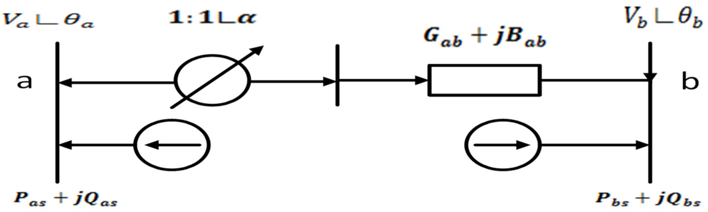
3.1. Model of Thyristor-Controlled Series Compensator Phase Shifter (TCSC)

TCSC is one of the most effective and extensively utilized FACTS devices. In comparison to standard control devices, this device is mounted in series with a transmission line and provides smooth and flexible line-impedance control with significantly faster response; it has shown to be a good method for managing power flow particularly across lengthy transmission lines, where power angle control at either end is limited. Furthermore, the TCSC can be used to improve the electric network’s transient stability. Figure 1 depicts the TCSC’s basic circuit structure; it comprises of a thyristor-controlled reactor (XL) in parallel with a fixed series capacitor (XC). The TCSC is treated as a variable capacitive reactance by taking into account the reactance   X C < X L . Controlling the firing angle ( γ ) of the thyristors can change the inductive reactance. As a result, the effective reactance of TCSC can be stated as follows:
X TCSC ( γ ) = X C X L ( γ ) X L ( γ ) X C
Figure 2 depicts the TCSC static model fitted between buses a and b after adding TCSC. The transmission line’s modified reactance ( X eq ) is written as follows:
X eq = X ab X TCSC = ( 1 τ ) X ab
The degree of series compensation is referred to as follows:
τ = X TCSC X ab
where X ab is the line-inductive reactance. The power flow equations for the transmission line that includes TCSC are expressed as follows:
P ab = V 2 a G ab V a V b G ab Cos ( θ a θ b ) V a V b G ab Sin ( θ a θ b )
Q ab = V 2 a B ab V a V b B ab Sin ( θ a θ b ) + V a V b B ab Cos ( θ a θ b )
P ba = V 2 b G ab V a V b G ab Cos ( θ a θ b ) + V a V b G ab Sin ( θ a θ b )
Q ba = V 2 b B ab + V a V b B ab Sin ( θ a θ b ) + V a V b B ab Cos ( θ a θ b )
G ab = R ab R 2 ab + [ ( 1 τ ) X mn ] 2
B ab = ( 1 τ ) X ab R 2 ab + [ ( 1 τ ) X mn ] 2

3.2. Model of Thyristor-Controlled Phase Shifter (TCPS)

Figure 3 shows the TCPS model fitted between the transmission lines that connect buses a and b, and the equations for the line’s power flow are as follows:
P ab = V 2 a G ab Cos 2 α V a V b Cos α [ G ab Cos ( σ a σ b + α ) + B ab Sin ( σ a σ b + α ) ]
Q ab = V 2 a B ab Cos 2 α V a V b Cos α [ G ab   Sin   ( σ a σ b + α ) + B ab Cos   ( σ a σ b + α ) ]
P ba = V 2 b G ab V a V b Cos α [ G ab   Cos   ( σ a σ b + α ) + B ab Sin   ( σ a σ b + α ) ]
Q ba = V 2 b B ab V a V b Cos α [ G ab   Sin   ( σ a σ b + α ) + B ab   Cos   ( σ a σ b + α ) ]
At bus a and bus b, TCPS injects actual and reactive power, expressed as follows:
P as = G ab V 2 b   Tan 2 α V a V b Tan   α   [ G ab   Sin   ( σ a σ b ) B ab   Cos   ( σ a σ b ) ]
Q as = B ab V 2 b   Tan 2 α + V a V b Tan   α   [ G ab   Cos   ( σ a σ b ) + B ab   Sin   ( σ a σ b ) ]
P bs = V a V b Tan   α   [ G ab   Sin   ( σ a σ b ) + B ab   Cos   ( σ a σ b ) ]
Q bs = V a V b Tan   α   [ G ab   Cos   ( σ a σ b ) B ab   Sin   ( σ a σ b ) ]

3.3. The Model of Static var Compensator (SVC)

In electric power systems, SVC is utilized to provide quick operational reactive power control; they control electric variables affecting the power grid quickly using a mix of capacitors and reactors for a variety of reasons. They are used in electric power systems, and one of the most important is quick voltage management at network weak points. SVC is coupled in a thyristor-controlled reactor ( X L c e r e e c t i v e l y d   i n   a   T h y r i s t o r = ω C ) with fixed capacitor X C c e r e e c t i v e l y d   i n   a   T h y r i s t o r = 1 ω C (TCR-FC). Set up in its most basic version, SVC can be used for inductive as well as capacitive correction. Figure 4 and Figure 5 depict the TCR-FC standard diagram and equivalent circuit, respectively.
The equivalent susceptibility is determined by the following formula:
B S V C = B C + B L ( γ )
where
B C = w C       a n d     B L ( γ ) = 1 w L ( 1 2 γ π S i n 2 γ π )
SVC provides reactive power, which may be represented as follows in terms of power flow:
Q S V C = V 2 m B S V C

4. Objective of Optimization

In this paper, the researcher proposed the modified electric network IEEE 30-bus as a test case that contains 30 bus; 41 branches [42]; 4 thermal generators at buses 1, 2, 8, and 13; and the 2 thermal generators at buses 5 and 11 are replaced by wind generator. Moreover, three FACTS devices are preferred and placed at an optimal location with appropriate ratings, namely SVC, TCSC, and TCPS.
  • Total costs of generation
The fundamental goal of optimum power flow is to be formulated containing all the costs in the modified system, which is illustrated as follows:
C T o t ( g ) = j = 1 N T C T 2 j ( P T G j ) + i N w [ C d i ( P w s c i ) + C R e w i ( P w s c i P w a v i ) + C P e w i ( P w a v i P w s c i ) ]
where N T is the thermal generation number, and N w is the wind generation number.
  • Active power losses
In the OPF issue, the network parameters, such as voltage deviation and active power loss in the transmission line of the system, are very important. The network active power loss is estimated as
P L = d = 1 N b G d ( a b ) [ V 2 a + V 2 b 2 V a V b   C o s ( σ a b ) ]
where σ a b = σ a σ b is the difference in voltage angles between buses a and b, and σ a b is transferred conductance of the line between a and b; N b is the number of transmission lines.
  • Voltage deviation
In addition, by decreasing the voltage deviation of all load buses, we improve the voltages at all load busses by considering the constraint control, which will help to make the network more stable and reliable. The voltage deviation is estimated mathematically as follows:
V D = a = 1 N L ( | V L a 1 | )
where N L is the number of loaded buses.

4.1. Equality and Inequality Constraints

4.1.1. Operational Equality Constraints

Equality constraints are the power balance equations where the generated active and reactive power in the electrical system is equal to the loads, and power losses in cases without FACTS devices in the network can be defined as follows:
P g a P d a V a N = 1 N b V b γ a b C o s ( a b + σ a σ b ) = 0
Q g a Q d a V a N = 1 N b V b γ a b S i n ( a b + σ a σ b ) = 0
where N b is the number of busses, P g a and Q g a are the generated active and reactive power, while P d a and Q d a are the active and reactive load at bus a, and a b is the difference in the angle of the admittance matrix.
In addition, the power balance in case of integrating FACTS devices can be defined as
P g a + P a s P d a V a N = 1 N b V b γ a b C o s ( a b + σ a σ b ) = 0
Q g a + Q a s Q d a Q S V C a V a N = 1 N b V b γ a b S i n ( a b + σ a σ b ) = 0
where P a s is the generated real power, Q a s is the reactive power incorporated by the TCPS, and Q S V C a is the reactive power incorporated by SVC.

4.1.2. Operational Inequality Constraints

The inequality constraints include the three restrictions listed below:
  • Generator constraints:
Active, reactive, and voltage of the generator lay between upper and lower boundaries as follows:
P g j m i n   P g j   P g j m a x                                               j N ( g e n )
Q g j m i n   Q g j   Q g j m a x                                         j N ( g e n )
V gj min   V gj   V gj max                  j N ( gen )
  • Transformer tap setting constraints:
Transformer tap setting (T) must be between lower and upper boundaries as shown below:
T s m i n   T s   T s m a x                                               s N ( T r )
where N ( T r ) is the number of transformers.
  • FACTS devices constraints:
    T C S C   :   τ T C S C a m i n   τ T C S C a   τ T C S C a m a x                                               a N ( T C S C )
    T C P S   :   τ T C P S a m i n   τ T C P S a   τ T C P S a m a x                                               a N ( T C P S )
    S V C   :   Q S V C i m i n   Q S V C i   Q S V C i m a x                                               i N ( S V C )
    where N ( T C S C ) , N ( T C P S ) , and N ( S V C ) are the numbers of FACTS devices.

5. Modified Moth–Flame Optimization and Gradient-Based Optimizer (GBO-MFO)

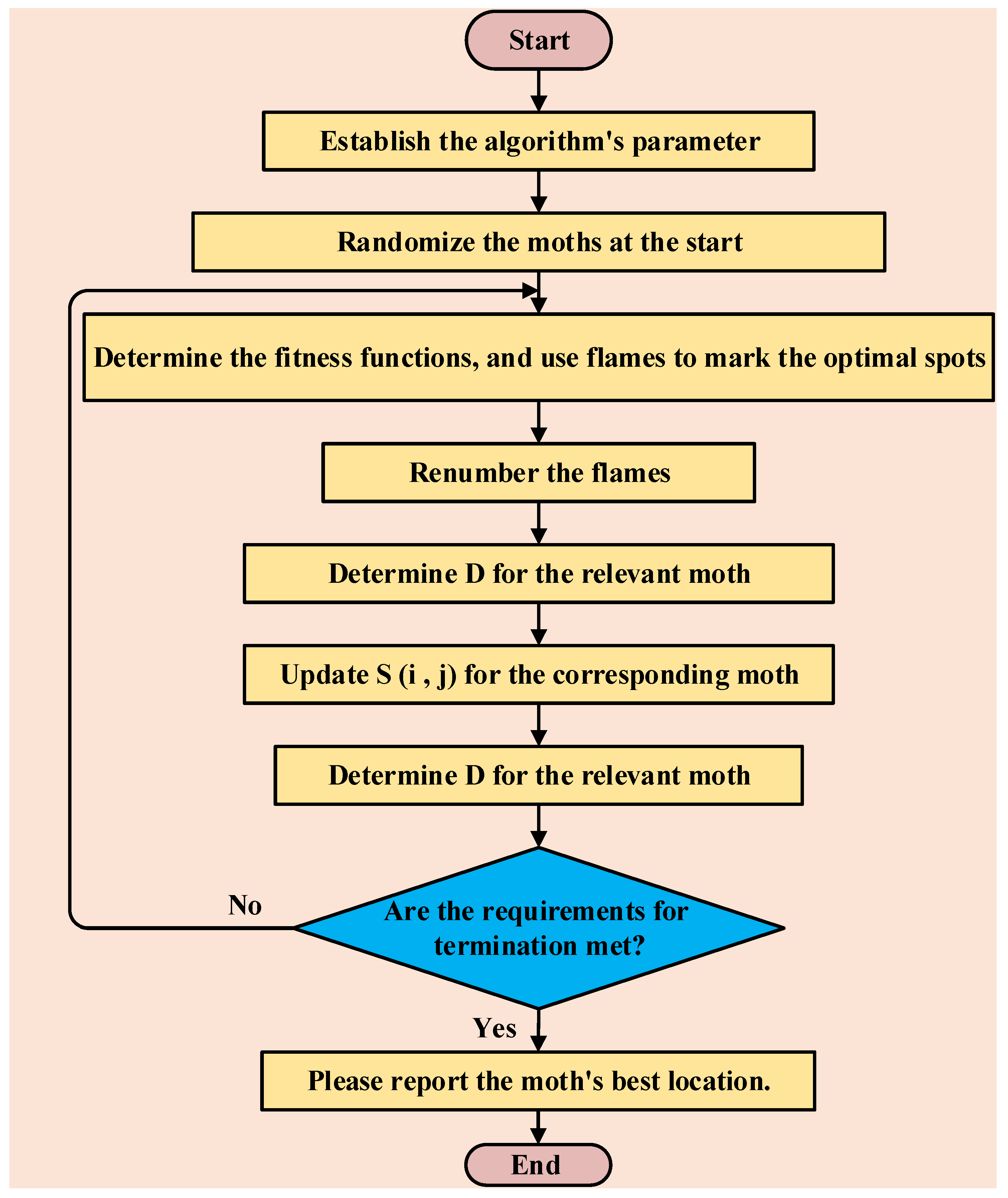
5.1. Moth–Flame Optimization (MFO) Algorithm

MFO was suggested by Mirjalili in [43]. MFO begins by producing moths at random in the solution space, as shown in the flow chart in Figure 6, and then estimating each moth’s fitness values and labeling the optimal position with flame; the moths’ positions are then updated using a spiral movement function to improve the flame-marked spots and to update the new best individual places and continuing the preceding procedures (the locations of the moths are being updated, and new ones are being created) until the termination requirements are reached.
There are three steps in the MFO technique corresponding to the measurements to take, which are as follows below.

5.1.1. Creating the Initial Moth Population

Each moth, according to Mirjalili in [43], can fly in one of four dimensions; moths can be expressed as a group as follows:
S = [ S 1 , 1 S 1 , 2 S 2 , 1 S 22 S 1 , m S 2 , m S n , 1 S n , 2 S n , m ]
where n denotes the number of moths in the search space, and m denotes the number of dimensions. In addition, all moth fitness values are memorized as
O S = [ O S 1 O S 2 O S n ]
Flames make up the remaining components of the MFO algorithm. In three-dimensional space, the flames along with their fitness function vector are shown in the following matrix below:
A = [ A 1 , 1 A 1 , 2 A 2 , 1 A 22 A 1 , m A 2 , m A n , 1 A n , 2 A n , m ]
O A = [ O A 1 O A 2 O A n ]

5.1.2. Positions of the Moths Are Being Updated

To find the global best solution for the optimization issues, MFO uses three separate functions. The following are the definitions for these functions:
M F O = ( I , P , T )
where I denotes the moths’ initial random locations, P denotes the moths’ mobility in the search space, and T denotes the end of the search process. The I function, which is utilized to implement the random distribution, is represented by using the following formula:
S ( i , j ) = ( U P ( i ) L P ( j ) r a n d ( i ) ) + L P ( i )
where the lower and upper boundaries of variables are denoted by UP and LP, respectively.
The moths use a transverse orientation to fly through the search space, as previously stated. When working with a logarithmic spiral, there are three things to keep in mind:
  • The moth should be the initial point on the spiral.
  • The flame’s location should be the spiral’s termination point.
  • The range of the spiral should not fluctuate beyond the search space.
As a result, the MFO algorithm’s logarithmic spiral is
W ( S i , A j ) = C i e b t C o s ( 2 π t ) + A j
C i denotes the distance between the i-th moth and the j-th flame, b provides a fix to determine the logarithmic spiral’s shape, and t is a random number between (−1,1). The spiral motion of the moth towards the flame in the search zone in MFO ensures a balance between exploitation and exploration.

5.1.3. Updating the Number of Flames

This section focuses on enhancing the exploitation of the MFO method (for example, updating the moths’ positions in n distinct locations in the search space may minimize the risk of exploiting the most promising solutions). As a result, reducing the number of flames aids in the resolution of this problem as shown by the equation below:
N o . f l a m e = r o u n d ( N l N l T )
where N represents the maximum number of flames, l represents the current number of iterations, and T represents the maximum number of iterations.

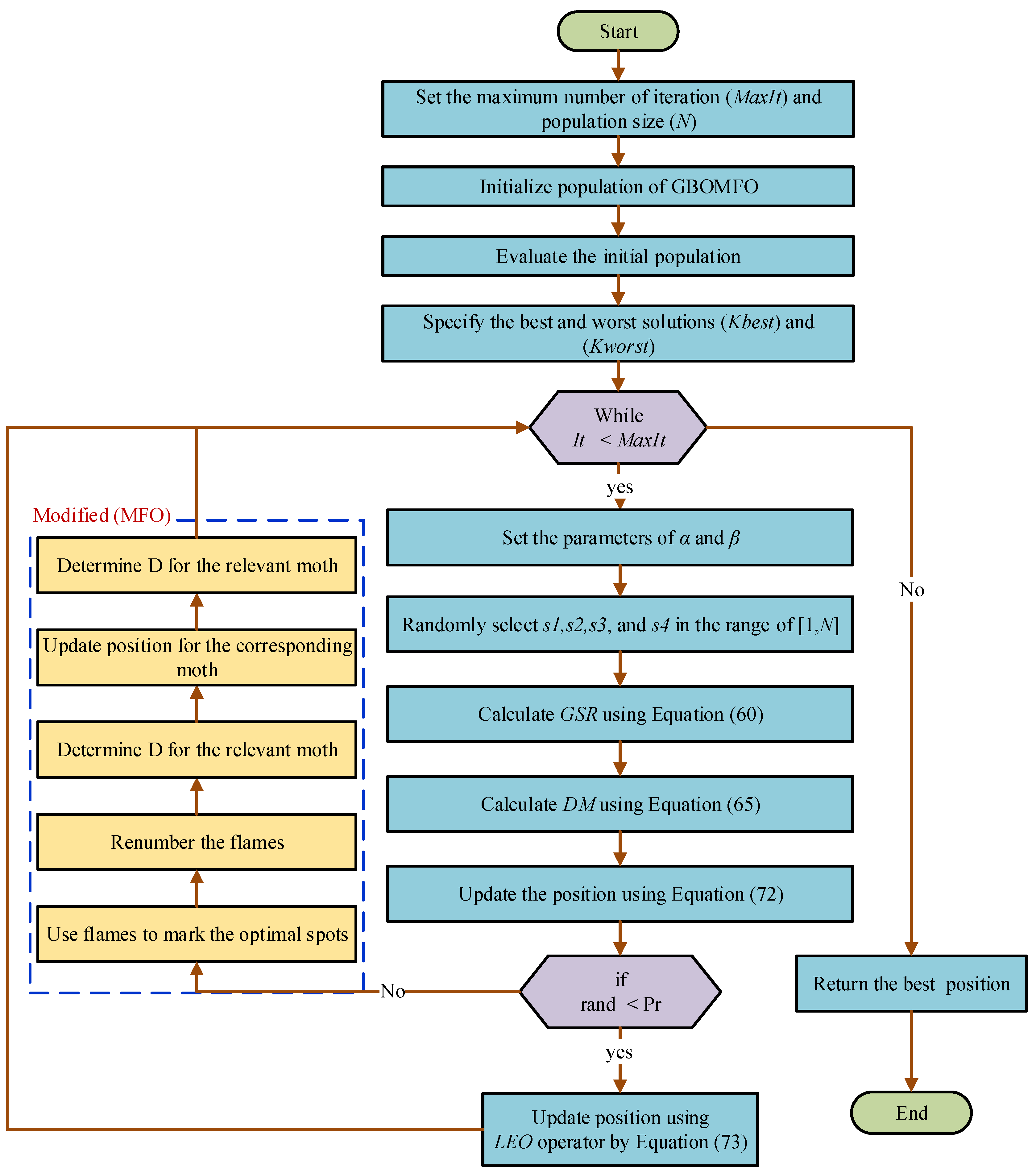
5.2. Gradient-Based Optimizer (GBO)

The suggested GBO [44] combines gradient and population-based approaches, and it utilizes the Newton’s technique, which specifies the search direction to investigate the search domain with the use of a collection of vectors and two primary operators, namely gradient search rule and local escaping operators.

5.2.1. Initialization Process

β = β min + ( β max β min ) ( 1 ( h H ) 3 ) 2
A set of choice variables, restrictions, and a goal-oriented function are all part of an optimization issue, and the probability rate and the parameters for transition between exploration and exploitation are among the GBO’s control parameters. Each person of the population is known as a “vector” in the suggested algorithm. As a result, in a D-dimensional search space, the GBO contains NB vectors. As a result, a vector may be written in the following way:
K m , d = [ K m , 1 , K m , 2 , K m , D ] m = 1 , 2 , N d = 1 , 2 , D
K m = K min + rand ( 0 , 1 ) ( K max K min )
where K max ,   K min are the decision variable K limits, while rand (0, 1) is a random number in the range (0, 1).

5.2.2. Gradient Search Rule (GSR) Process

A significant factor called δ is used in the GBO algorithm to achieve a well-balanced search of a large area while yet attaining near-optimal and global results. The following is how the δ is used:
δ 1 = 2 rand α α
α = | β Sin ( 2 π 2 + sin ( β 2 π 2 ) ) |
where β min is a constant of 0.2, and β max is a constant of 1.2; h is the current iteration number, and H is the total number of iterations; the δ 1 parameter is in charge of balancing exploration and exploitation. Within a specific range, the parameter value rises via defined iterations. This broadens the range of possible answers and allows the algorithm to investigate different options. The GSR can be determined in the following way:
GSR = rand   m δ 1 2 Δ k k m ( k worst k best + σ )
In Equation (60), the random offset is defined as the distinction between the best and second-best solution ( k best ) and a randomly chosen solution ( k s 1 t ). The variable’s meaning changes as it is iterated Δ k , as seen by the Equation below (63). A second random number (rand n) is also given to enable further research as follows:
Δ K = rand ( 1 : N ) | step |
step = ( k best k s 1 t ) + ϑ 2
ϑ = 2 rand ( | k s 1 t + k s 2 t + k s 3 t + k s 4 t 4 k m t | )
where rand(1: N) is a random vector of N elements in the range of (0, 1). The four integers chosen at random are s 1 , s 2 , s 3 , and   s 4 such that s 1 s 2 s 3 s 4 m step represents a phase scale, which is represented by k best and k s 1 t . The term DM is calculated by taking given a set of potential vectors, the optimal vector, and transferring the current vector ( k m ) in the direction of the best vector ( k best k m ) as follows:
k m + 1 = k m GSR
DM = rand δ 2 ( k best k m )
δ 2 is a random parameter that is used to change the size of each vector agent’s phase, and it can be calculated as follows:
δ 2 = 2 rand α α
Finally, DM and GSR can be modified as
K 1 m t = k 1 m t GSR + DM
where K 1 m t denotes the modified vector as a result of changing K 1 m t , and the transformation K 1 m t can be known as follows according to Equations (55) and (65):
K 1 m t = k m t rand   m δ 1 2 Δ k k m t ( yP m t yP m t + σ ) + rand δ 2 ( k best k m t )
where yP m t ,   yP m t are identical to y n + Δ k , and is equal to the average of two elements, A m + 1 ,   k m .
A m + 1 = k m rand   m 2 Δ k k m ( k worst k best + σ )
Despite the fact that k m represents the current solution, we get the present solution element K 2 m t by using the preceding procedure and replacing the present solution element k m t n with the new solution element k best .
K 2 m t = k best rand   m δ 1 2 Δ k k m t ( yP m t yP m t + σ ) + rand δ 2 ( k s 1 t k s 2 t )
Using Equation (68), the GBO method seeks to increase discovery and exploitation by making them more transportable than the last Equation (70), which is utilized to aid the local search’s exploitation phase. Finally, a revised version of the response available has been discovered, which is as follows:
k m t + 1 = s 1 ( s 2 K 1 m t + ( 1 s 2 ) K 2 m t ) + ( 1 s 1 ) K 3 m t )
where   s 1   and   s 2 are random numbers, and K 3 m t is presented as
K 3 m t = k m t + 1 δ 1 ( K 2 m t K 1 m t )

5.2.3. The Local Escaping Operator (LEO) Process

The LEO is a tool that may be used to improve an optimization’s performance method by assisting in the solution of complex engineering issues. The LEO operator aids the algorithm’s convergence by allowing it to easily move out of local optima positions. The LEO operator sets out to create a new solution that is a more efficient solution ( K LEO t ) by different solutions ( k best ); K 1 m t solutions are chosen randomly selected from the population, and k s 1 t ,   k s 2 t solutions are created at random. It efficiently upgrades current solutions and follows the following procedure:
If rand < P,
k LEO t { k m t + 1 + f 1 ( h 1 k best h 2 K e t ) + f 2 δ 1 ( h 3 ( K 2 m t K 1 m t ) ) h 3 ( k s 1 t k s 2 t ) / 2               if   rand < 0.5   k m t + 1 + f 1 ( h 1 k best h 2 K e t ) + f 2 δ 1 ( h 3 ( K 2 m t K 1 m t ) ) + h 3 ( k s 1 t k s 2 t ) / 2 ,    otherwise   
P is the value of probability, and P = 0.5 and h 1 ,   h 2 ,   and   h 3 are random created values as follows:
h 1 = { 2 rand           if   ω 1 < 0.5 1                                   otherwise
h 2 = { rand           if   ω 1 < 0.5 1                                   otherwise
h 3 = { rand           if   ω 1 < 0.5 1                                   otherwise
where rand is random number between (0, 1). The above values of h 1 , h 2 ,   and   h 3 can be reorganized as
h 1 = D 1 2 rand + ( 1 D 1 )
h 2 = D 1 rand + ( 1 D 1 )
h 3 = D 1 rand + ( 1 D 1 )
where D 1 is a binary vector takes a value of (0, 1); as an example, if parameter ω < 0:5, then, the value is D 1 ; otherwise, D 1 = 0 , where the answer k e t is created as follows:
k e t = { k rand           if   ω 2 = 0.5   k P t                           otherwise
K m is a random answer that is created using the formula below:
K m = K min + rand ( 0 , 1 ) ( K max K min )

5.3. Proposed GBO-MFO Algorithm

The original GBO algorithm suffers from the local optima when handling non-linear objective functions. Additionally, the convergence speed and precision are low because of the randomness. To overcome all these drawbacks and improve the solution efficiency as well as the rate of convergence, we proposed the GBO-MFO technique [45]. Figure 7 presents the flowchart of the suggested GBO-MFO algorithm. As shown in this Figure, the GBO is represented as the fundamental algorithm in the suggested hybrid algorithm. The GSR and LEO are used to update the place in the search space regarding the optimal solution in the original GBO. On the other hand, the original MFO takes use of the spiral movement ability to achieve the exploitation more than exploring the solution space [46]. The proposed algorithm is the hybridization of the GBO and MFO that owns the advantage of both algorithms.

6. Simulation Results and Discussion of the IEEE 30-Bus Test Network

As an example, the IEEE 30-bus electric network was utilized. The modified single-line diagram of IEEE 30-bus is presented in Figure 8. It has four thermal generators, two wind generators, and 24 load nodes. The major data and operational conditions of the test system are investigated in [42]. The electric network consists of four thermal generators at buses 1, 2, 8, and 13; two wind generators at buses 5 and 11; and four tap-changing transformers in branches 11, 12, 15, and 36. The voltage values of the PV nodes are within the boundaries of (0.95–1.1 p.u.). The tap transformers settings are considered within the range of (0.9–1.1 p.u.). In order to verify the strength of the proposed algorithm, GBO-MFO was implemented to solve the OPF issue with TCSC, SCPS, and SVC and practical limitations. The proposed technique is advanced in MATLAB 2014 programming circumference, and all sections of simulations have been coded in a PC with 2.40 GHZ frequency and the installed memory (RAM) is 4.0 GB. In this paper, the power flow is estimated by MATPOWER version 7 [47]. The electrical network loads are 283.4 MW and 126.2 MVar, and the main simulation results are presented in this section as shown in Table 2. The obtained results of the proposed hybrid GBO-MFO algorithm are compared with the results of four recent algorithms, including the gradient-based optimizer (GBO) [44], moth–flame optimization algorithm [43], slime mould algorithm (SMA) [48], and coulomb–franklin’s algorithm (CFA) [49]. The contol parameters of the proposed and others algorithms are illustrated in details in Table 3. This comparison with other modern meta-heuristic techniques is presented in Table 4. In the our optimization technique, the number of control variables are 27 as defined in detail in Table 4, which includs the locations and rating for each FACTS device, and while integrating the FACTS devices, some criteria must be considered, such as (1) only one FACTS device is put in the location, (2) SVC is not added on the PV bus, and (3) in case of line having tap transformer, TCSC and TCPS are not integrated into this lines. TCSC can compensate up to 50% of the branch reactance where it is placed, while SVC can provide or absorb up to 10 MVAr of reactive power. Phase shifter’s angle (TCPS) can be changed from −5 and 5. The case studies carried out under this section assume that the electric network is fully loaded; for the given full-loaded situation, three case studies are carried out, which are illustrated as follows:
  • Case A: Minimizing the cost generation.
  • Case B: Minimizing power losses.
  • Case C: Minimizing cost and power losses.
  • Case D: Load demand uncertainty
Case study findings using the GBO-MFO method are given in this part along with explanations. In each case study of optimization, each scenario was performed 30 times to determine the goal function’s most optimal value and the accompanying control variable settings.
  • Case A: Minimizing the Cost Generation
In Case A, it was observed that the electrical network total generation cost is greatly decreased to 807.12 ($/h) using GBO-MFO technique, which is less than the generation cost in Case B and Case C. Additionally, in this case, the minimum value of the voltage deviation was obtained. Because wind generators are less expensive, their scheduled power outputs are frequently higher than those of thermal units. However, because adequate wind energy is not available, a wind units’ output cannot be used to its most tremendous potential, as this will increase the reserve cost to provide scheduled power for extended periods of time.
The placements of FACTS devices as well as their ratings were adjusted in this article to reduce generating costs. In a genuine system or a variant of a well-known system, FACTS devices are installed without any research, which may result in wasteful and ineffective electric system resource consumption. In this case, buses 7 and 24 are considered to be the best sites for the SVCs, and TCSC was installed in branch 5 and branch 2, and TCPS was installed in branch 14 and branch 39.
In this paper, in all cases, we ran the technique multiple times after adjusting the optimal places to improve ratings while reducing costs. Due to the system’s heavy inductive load, SVC’s reactive power correction was nearly at its maximum. FACTS devices were placed in networks with the goal of improving loading capacity. The electrical network’s actual power loss was kept as low as possible in such a way as to optimize the capacity of the system’s loads. Furthermore, the suggested algorithm’s capacity was used to keep bus voltage amplitudes within a reasonable range. The state variables in the IEEE 30-bus test system ere kept within the allowed limits.
  • Case B: Minimizing power losses
The major goal of Case B was to lower active power loss to the absolute minimum. Many transmission lines in power networks result in significant active power loss. As a result, for large-scale systems, minimizing active power loss is critical. The GBO-MFO in Case B had the lowest active power loss.
In this case, the power losses achieved a minimal loss of 1.7467 MW using the control variables listed in Table 2. This value of power losses is better than Case A and Case C, and also the voltage deviation obtained in this case was 0.8622, and the emissions from traditional thermal power plants reached to 0.1416159. In this case, the SVCs were placed at buses 19 and 24, while the TCSC were placed at branches 34 and 41, and the two TCPS were installed at branches 35 and 14 given that reactive power in power networks is constantly distributed based on voltage magnitude differences between buses, resulting in a rise in power loss. This is a critical achievement, and it is also where the suggested algorithm’s effect is scrutinized. As an example, one of the most visible aims of the OPF issue is to keep the numerical value of voltage values of the buses between their borders and around typical operating circumstances.
Constraints on load bus voltage are particularly important in the OPF issue since the voltages at which load buses operate are frequently found to be near to their limitations, which must be kept between 0.95 and 1.05 p.u. in our investigation. Furthermore, the limits on reactive power of generators are also met in all situations.
  • Case C: Minimizing cost and power losses
Through the comparison presented in Table 2, we found that the cost of generation in Case A is less than the cost of generation in Case B, while the reduction in power losses in Case B is better than in Case A. This statistic emphasizes the need to have a goal that includes both of them, which forced us to resort to the use of Case C. Developing a cost model in which the loss is translated into an equal price of energy is a straightforward method to account for both objectives. The cost of electricity used in this research is $0.10 per kWh. The cost of power was $0.10 per kWh in this research as presented in Equation (82).
C Gross = C T o t ( g ) + P L 10 3 0.10 )
In Case C, the technique’s minimal goal value is 1104.0771 $/h, and the active power loss is 1.87682 MW, total generation cost is 916.65170 $/h, voltage deviation is 0.8347 p.u., and the emission is 0.14196. The two SVCs were installed at busses 24 and 21 and the two TCSC at branches 2 and 9, while the two TCPS WERE placed at branches 33 and 5. In this case, the best cost and loss values WERE determined by the coefficient of price chosen for generators, including thermal and wind. However, taking into account both goals results in the lowest total cost.
  • Case D: Load demand uncertainty
In OPF research studies, determination of FACTS devices placement and rating considering uncertainties in load demands is a well-developed research topic. The research scenario discussed in this section considers a genuine incident of changing load. The probability density function (PDF) [45] WAS used to depict the unpredictablity of demands. It Is worth noting that this technique also optimizes the placement of the FACTS, and also changing the placement of FACTS during various loading circumstances is not possible as a result, so the FACTS were carefully located for a particular scenario with the greatest chance of occurring. The probability of Scenario 3 and Scenario 4 occurring is the greatest. We improved the positions of the FACTS devices for Scenario 3, and its same optimal placement was used to optimize the FACTS for other scenarios. In addition, the values of the FACTS devices used were adjusted to account for various system scenarios; the research is useful since it optimizes a variety of electrical system aims by executing OPF at regular intervals. The normal distribution with mean μ d and standard deviation α d is commonly used to model the load demand uncertainty and are 70 and 10, respectively. In this work, all loads are assumed to obtain the same PF, mean, and standard deviation. As a result, rather than using a normal distribution to every load separately, Δ S , j shows the probability of each load level that is computed by Equation (83); Equation (84) can also be used to calculate the related value of every load level, which is indicated by P d , i ¯ .
These formulas [50] are used to compute the mean load and probability of an event for a given case.
Δ S , j = P d , j M i n P d , j M a x 1 α d 2 π   exp [ ( P d μ d ) 2 2 α d 2 ] d P d
where P d , j M a x and P d , j M i n are the maximum and minimum boundaries of ith scenarios of loading, and the mean of ith scenarios of load demand is
P d , i ¯ = 1 Δ S , j P d , j M i n P d , j M a x ( P d 1 α d 2 π exp [ ( P d μ d ) 2 2 α d 2 ] d P d )
Additionally, for the premeditated medians and probability for any and all possible load-carry situations, the percent load in a situation means that the nodes needs are multiplied by the % of that scenario. As a result, the technique optimized the performance index of gross cost as written in (82) under various conditions, and the active power generated from all generators was used at full capacity in every scenario.
The variable’ limits, such as the limits presented in Table 2 and Table 4, present effective system parameters for the four scenarios, which show the best amplitude of gross cost. For all scenarios, the expected gross cost is determined as follows:
EGRC = SC = 1 NO SC Δ SC C gross , sc
where NO SC is the scenario’s number. Δ SC is the scenario’s probability, which is estimated in Table 5. EGC is the expected generation cost, and EPL is expected power loss, which is estimated in [51] and computed by
E G C = S C = 1 N O S C Δ S C C G e n ,     s c
E P L = S C = 1 N O S C Δ S C P L o s s , s c

7. Discussion

The numerical results show that, when compared to previous techniques in the literature, such as GBO, MFO, SMA, and CFA, the suggested methodology provides a better and more acceptable solution for handling various versions of the OPF issue while taking into account realistic limitations and FACTS devices. The proposed technique GBO-MFO became stuck in local optima quite fast, and it may converge to a superior solution in less iterations as presented in Figure 9 for Case A, Figure 10 for Case B, and Figure 11 for Case C, unlike the other techniques investigated in this study. For more knowledge, consider Case 1, a well-known case study in the field of OPF problem-solving. The most talented generation cost achieved by the suggested method when FACTS devices are taken into account is 807.12 ($/h). These numbers are lower than those of the other techniques evaluated and those found in the paper, which are 807.2502 ($/h) in GBO and 807.469 in CFA, 807.277 in SMA, and 807.4733 in MFO. It is worth noting that a successful optimization method not only converges to a reduced total generation cost while solving the OPF issue, but it also reduces active power losses. Additionally, the power loss is 5.56 MW in the proposed method, which is better than 5.60, 5.62, 5.57, and 5.6304 in GBO, CFA, SMA, and MFO, respectively.
Figure 12 shows a bar chart depicting the breakdown of different costs; because of the tiny cost coefficient for penalties, the cost of not using obtainable wind energy is minimal in all circumstances. Generator units linked to buses 5, 8, and 11 are necessary in Cases B and C to decrease power losses because system loading in the area is extremely high; therefore, it should run at or near its rated capacity. The reserve cost in Cases B and C increases as the planned power from the wind turbines increases. Because the direct cost is related to its anticipated output, it rises as the scheduled power grows. As a result of the reduced scheduled power of the thermal units, the cost of these units decreases in Cases B and C compared to Case A. The cost of loss is calculated using the energy unit cost. When the power loss is included as a goal in the optimization, the cost is properly reduced.
Likewise, in the Cases B and C, the ideal settings of the generator units’ active power are shown below in Figure 13 for Cases A to C. Figure 14 shows the voltage of load buses of the case studies for the modified system when it is fully loaded. For Cases A to C, the best settings of voltages on the generator bus are presented in Figure 15, and Figure 16 also explains the setting of the transformer tap ratio for Case A to Case C This demonstrates the effectiveness of the suggested approach, which is capable of achieving the best global value with fewer rounds.
Table 6 contains the obtained results of using the Wilcoxon signed rank test. The proposed GBO-MFO algorithm is compared with four well-known algorithms in the literature, including GBO, MFO, CFA, SMA, respectively, for the Cases A, B, and C.
In case of loading scenarios, the system costs and active power losses are significantly reduced, as presented in Table 7, because of their permanent placements, which are optimized depending on Scenario 3, the FACTS compensate in a major way across all scenarios. In addition, as shown in Case C, the optimal planned power in buses 5, 8, and 11 rise as system loading rises. Furthermore, with the variation in loads, the power of generator units is nearly unaffected. The requirement to reduce to reduce system active power loss is the primary reason behind this. Figure 17 presents the convergence characteristics for different loading scenarios in Case D, and Figure 18 depicts the voltages for each scenario and the upper and lower limits.

8. Conclusions

This study provides a technique to achieve optimal power flow. In the IEEE 30-bus network, there is an issue involving stochastic wind and FACTS devices (OPF), and the suggested MFO-GBO was successfully applied to solve the OPF problem in electric power network. In the three case studies, the placement and rating of the FACTS devices (SVC, TCSC, and TCPS) were optimized with the goal of decreasing generation cost and active power loss in the electric network system. The necessity of considering both factors together demonstrated a composite target that includes generation cost and active power loss. The electric network power loss is translated to an energy cost as well as the expense of production. The MFO-GBO was proven to provide a rapid, accurate, and optimal solution to the OPF issue. The MFO-GBO was contrasted and analyzed for calculating the best set of control variables on IEEE 30-bus to examine the efficacy and superiority of the proposed algorithms to keep generation costs down, decrease power losses to minimum value, and enhance the voltage profile. In addition, MFO-GBO was provided to solve the OPF issue considering uncertain load demand. The collected findings demonstrate the proposed approach’s advantage in obtaining the best solution with the shortest time to convergence. These findings support its efficacy in resolving large-scale OPF issues. The suggested technique outperforms existing in terms of well-known optimization techniques computing performance.

9. Future Recommendation

For future OPF study, the authors recommend incorporating tiny hydro-generators and storage in the form of battery or hydro power in a large system. FACTS devices can be used to create a realistic model of doubly-fed induction generators for wind generators.

Author Contributions

Conceptualization, A.A.M., S.K. and M.H.H.; Data curation, M.A. and M.I.M.; Formal analysis, A.A.M., S.K. and M.H.H.; Software, M.A. and M.I.M.; Investigation, A.A.M., S.K. and M.H.H.; Methodology, A.A.M., S.K. and M.H.H.; Project administration, M.A. and M.I.M.; Resources, M.A. and M.I.M.; Software, A.A.M., S.K. and M.H.H.; Supervision, S.K., M.A. and M.I.M.; Validation, S.K. and M.H.H.; Visualization, M.A. and M.I.M.; Writing original draft, A.A.M., S.K. and M.H.H.; Writing—review & editing, M.A. and M.I.M. All authors have read and agreed to the published version of the manuscript.

Funding

The research received no external funding.

Institutional Review Board Statement

Not applicable.

Informed Consent Statement

Not applicable.

Data Availability Statement

Not applicable.

Acknowledgments

The authors thank the support of the National Research and Development Agency of Chile (ANID), ANID/Fondap/15110019.

Conflicts of Interest

The authors declare no conflict of interest.

References

  1. Lee, K.; Park, Y.; Ortiz, J. A united approach to optimal real and reactive power dispatch. IEEE Trans. Power App. Syst. 1985, 104, 1147–1153. [Google Scholar] [CrossRef]
  2. Alsaç, O.; Bright, J.; Prais, M.; Stott, B. Further developments in LP-based optimal power flow. IEEE Trans. Power Syst. 1990, 5, 697–711. [Google Scholar] [CrossRef]
  3. Momoh, J.A.; El-Hawary, M.E.; Adapa, R. A review of selected optimal power flow literature to 1993. II. Newton, linear programming and interior point methods. IEEE Trans. Power Syst. 1999, 14, 105–111. [Google Scholar] [CrossRef]
  4. He, S.; Wen, J.Y.; Prempain, E.; Wu, Q.H.; Fitch, J.; Mann, S. An improved particle swarm optimization for optimal power flow. In Proceedings of the International Conference on Power System Technology (POWERCON), Singapore, 21–24 November 2004; pp. 1633–1637. [Google Scholar]
  5. Abido, M.A. Optimal power flow using tabu search algorithm. Electr. Power Compon. Syst. 2002, 30, 469–483. [Google Scholar] [CrossRef] [Green Version]
  6. Yan, X.; Quintana, V.H. Improving an interior-point-based off by dynamic adjustments of step sizes and tolerances. IEEE Trans. Power Syst. 1999, 14, 709–716. [Google Scholar]
  7. Olofsson, M.; Andersson, G.; Soder, L. Linear programming based optimal power flow using second order sensitivities. IEEE Trans. Power Syst. 1995, 10, 1691–1697. [Google Scholar] [CrossRef]
  8. Sun, D.I.; Ashley, B.; Brewer, B.; Hughes, A.; Tinney, W.F. Optimal power flow by Newton approach. IEEE Trans. Power App. Syst. 1984, PAS-103, 2864–2880. [Google Scholar] [CrossRef]
  9. Roy, P.K.; Paul, C. Optimal power flow using krill herd algorithm. Int. Trans. Electr. Energy Syst. 2015, 25, 1397–1419. [Google Scholar] [CrossRef]
  10. Mohamed, A.-A.A.; Mohamed, Y.S.; El-Gaafary, A.A.M.; Hemeida, A.M. Optimal power flow using moth swarm algorithm. Electr. Power Syst. Res. 2017, 142, 190–206. [Google Scholar] [CrossRef]
  11. Mahdad, B.; Srairi, K. Blackout risk prevention in a smart grid based flexible optimal strategy using Grey Wolf-pattern search algorithms. Energy Convers. Manag. 2015, 98, 411–429. [Google Scholar] [CrossRef]
  12. El-Fergany, A.; Hasanien, H.M. Salp swarm optimizer to solve optimal power flow comprising voltage stability analysis. Neural Comput. Appl. 2019, 32, 5267–5283. [Google Scholar] [CrossRef]
  13. Hassan, M.H.; Kamel, S.; Selim, A.; Khurshaid, T.; Domínguez-García, J.L. A modified Rao-2 algorithm for optimal power flow incorporating renewable energy sources. Mathematics 2021, 9, 1532. [Google Scholar] [CrossRef]
  14. Naderi, E.; Pourakbari-Kasmaei, M.; Cerna, F.V.; Lehtonen, M. A novel hybrid self-adaptive heuristic algorithm to handle single-and multi-objective optimal power flow problems. Int. J. Electr. Power Energy Syst. 2021, 125, 106492. [Google Scholar] [CrossRef]
  15. Abido, M.A. Optimal power flow using particle swarm optimization. Int. J. Electr. Power Energy Syst. 2002, 24, 563–571. [Google Scholar] [CrossRef]
  16. Roa-Sepulveda, C.A.; Pavez-Lazo, B.J. A solution to the optimal power flow using simulated annealing. Int. J. Electr. Power Energy Syst. 2003, 25, 47–57. [Google Scholar] [CrossRef]
  17. Bouktir, T.; Slimani, L.; Belkacemi, M. A genetic algorithm for solving the optimal power flow problem. Leonardo J. Sci. 2004, 4, 44–58. [Google Scholar]
  18. Mukherjee, A.; Mukherjee, V. Solution of optimal power flow using chaotic krill herd algorithm. Chaos Solitons Fract. 2015, 78, 10–21. [Google Scholar] [CrossRef]
  19. Kaymaz, E.; Duman, S.; Guvenc, U. Optimal power flow solution with stochastic wind power using the Lévy coyote optimization algorithm. Neural Comput. Appl. 2020, 33, 6775–6804. [Google Scholar] [CrossRef]
  20. Yunus, A.M.S.; Abu-Siada, A.; Mosaad, M.I.; Albalawi, H.; Aljohani, M.; Jin, J.X. Application of SMES Technology in Improving the Performance of a DFIG-WECS Connected to a Weak Grid. IEEE Access 2021, 9, 124541–124548. [Google Scholar] [CrossRef]
  21. Mosaad, M.I.; Alenany, A.; Abu-Siada, A. Enhancing the performance of wind energy conversion systems using unified power flow controller IET Generation. Transm. Distrib. 2020, 14, 1922–1929. [Google Scholar] [CrossRef]
  22. Panda, A.; Tripathy, M. Security constrained optimal power flow solution of wind-thermal generation system using modified bacteria foraging algorithm. Energy 2015, 93, 816–827. [Google Scholar] [CrossRef]
  23. Marley, J.F.; Vrakopoulou, M.; Hiskens, I.A. An AC-QP optimal power flow algorithm considering wind forecast uncertainty. In Proceedings of the Innovative Smart Grid Technologies-Asia (ISGT-Asia), Melbourne, Australia, 28 November–1 December 2016; pp. 317–323. [Google Scholar]
  24. Mosaad, M.I.; Ramadan, H.S.; Aljohani, M.; Sherif, M.F.E.; Ghoneim, S.S.M. Near-Optimal PI Controllers of STATCOM for Efficient Hybrid Renewable Power System. IEEE Access 2021, 9, 34119–34130. [Google Scholar] [CrossRef]
  25. Mosaad, M.I.; Sabiha, N.A. Ferroresonance Overvoltage Mitigation using STATCOM for Grid-Connected Wind Energy Conversion Systems. J. Mod. Power Syst. Clean Energy 2021, 1–9. [Google Scholar]
  26. Nusair, K.; Alasali, F.; Hayajneh, A.; Holderbaum, W. Optimal placement of FACTS devices and power-flow solutions for a power network system integrated with stochastic renewable energy resources using new metaheuristic optimization techniques. Int. J. Energy Res. 2021, 45, 18786–18809. [Google Scholar] [CrossRef]
  27. Rambabu, M.; Nagesh Kumar, G.V.; Sivanagaraju, S. Optimal power flow of integrated renewable energy system using a thyristor controlled SeriesCompensator and a grey-wolf algorithm. Energies 2019, 12, 2215. [Google Scholar] [CrossRef] [Green Version]
  28. Inkollu, S.R.; Kota, V.R. Optimal setting of FACTS devices for voltage stability improvement using PSO adaptive GSA hybrid algorithm. Eng. Sci. Technol. Int. J. 2016, 19, 1166–1176. [Google Scholar] [CrossRef] [Green Version]
  29. Mukherjee, A.; Mukherjee, V. Solution of optimal power flow with FACTS devices using a novel oppositional krill herd algorithm. Int. J. Electr. Power Energy Syst. 2016, 78, 700–714. [Google Scholar] [CrossRef]
  30. Pandiarajan, K.; Babulal, C.K. Fuzzy Harmony search algorithm based optimal power flow for power system security enhancement. Int. J. Electr. Power Energy Syst. 2016, 78, 72–79. [Google Scholar] [CrossRef]
  31. Rao, B.V.; Nagesh-Kumar, G.V. Optimal power flow by BAT search algorithm for generation reallocation with unified power flow controller. Int. J. Electr.Power Energy Syst. 2015, 68, 81–88. [Google Scholar]
  32. Acharjee, P. Optimal power flow with UPFC using security constrained self a adaptive differential evolutionary algorithm for restructured power system. Int. J. Electr. Power Energy Syst. 2016, 76, 69–81. [Google Scholar] [CrossRef]
  33. Prasad, D.; Mukherjee, V. A novel symbiotic organism’s search algorithm for optimal power flow of power system with FACTS devices. Eng. Sci. Technol. Int. J. 2016, 19, 79–89. [Google Scholar]
  34. Rahman, J.; Feng, C.; Zhang, J. A learning-augmented approach for AC optimal power flow. Int. J. Electr. Power Energy Syst. 2021, 130, 106908. [Google Scholar] [CrossRef]
  35. Abd El-sattar, S.; Kamel, S.; Ebeed, M.; Jurado, F. An improved version of salp swarm algorithm for solving optimal power flow problem. Soft Comput. 2021, 25, 4027–4052. [Google Scholar] [CrossRef]
  36. Su, Q.; Khan, H.U.; Khan, I.; Choi, B.J.; Wu, F.; Aly, A.A. An optimized algorithm for optimal power flow based on deep learning. Energy Rep. 2021, 7, 2113–2124. [Google Scholar] [CrossRef]
  37. Shilaja, C. In Perspective of Combining Chaotic Particle Swarm Optimizer and Gravitational Search Algorithm Based on Optimal Power Flow in Wind Renewable Energy. In Soft Computing Techniques and Applications; Springer: Singapore, 2021; pp. 477–490. [Google Scholar]
  38. Ehsan, N.; Mahdi, P.; Hamdi, A. An efficient particle swarm optimization algorithm to solve optimal power flow problem integrated with FACTS devices. Appl. Soft Comput. J. 2019, 80, 243–262. [Google Scholar]
  39. Biswas, P.P.; Suganthan, P.N.; Amaratunga, G.A.J. Optimal power flow solutions incorporating stochastic wind and solar power. Energy Convers. Manag. 2017, 148, 1194–1207. [Google Scholar] [CrossRef]
  40. Biswas, P.P.; Suganthan, P.N.; Qu, B.Y.; Amaratunga, G.A.J. Multiobjective economic-environmental power dispatch with stochastic wind-solar-small hydro power. Energy 2018, 150, 1039–1057. [Google Scholar] [CrossRef]
  41. Biswas, P.P.; Suganthan, P.N.; Mallipeddi, R.; Amaratunga, G.A.J. Optimal power flow solutions using differential evolution algorithm integrated with effective constraint handling techniques. Eng. Appl. Artif. Intell. 2018, 68, 81–100. [Google Scholar] [CrossRef]
  42. Alsac, O.; Stott, B. Optimal Load Flow with Steady-State Security. IEEE Trans. Power Appar. Syst. 1974, PAS-93, 745–751. [Google Scholar] [CrossRef] [Green Version]
  43. Mirjalili, S. Moth-flame optimization algorithm: A novel nature-inspired heuristic paradigm. Knowl.-Based Syst. 2015, 89, 228–249. [Google Scholar] [CrossRef]
  44. Ahmadianfar, I.; Bozorg-Haddad, O.; Chu, X. Gradient-based optimizer: A new metaheuristic optimization algorithm. Inf. Sci. 2020, 540, 131–159. [Google Scholar] [CrossRef]
  45. Premkumar, M.; Jangir, P.; Ramakrishnan, C.; Nalinipriya, G.; Alhelou, H.H.; Kumar, B.S. Identification of solar photovoltaic model parameters using an improved gradient-based optimization algorithm with chaotic drifts. IEEE Access 2021, 9, 62347–62379. [Google Scholar] [CrossRef]
  46. Rajeshkumar, G.; Sujatha, T.P. Optimal positioning and sizing of distributed generators using hybrid MFO-WC algorithm. J. Comput. Mech. Power Syst. Control 2019, 2, 19–27. [Google Scholar] [CrossRef]
  47. Zimmerman, R.D.; Murillo-Sánchez, C.E. Matpower (Version 7.0). 2019. Available online: https://matpower.org (accessed on 10 December 2021).
  48. Li, S.; Chen, H.; Wang, M.; Heidari, A.A.; Mirjalili, S. Slime mould algorithm: A new method for stochastic optimization. Future Gener. Comput. Syst. 2020, 111, 300–323. [Google Scholar] [CrossRef]
  49. Ghasemi, M.; Ghavidel, S.; Aghaei, J.; Akbari, E.; Li, L. CFA optimizer: A new and powerful algorithm inspired by Franklin’s and Coulomb’s laws theory for solving the economic load dispatch problems. Int. Trans. Electr. Energy Syst. 2018, 28, e2536. [Google Scholar]
  50. Mohseni-Bonab, S.M.; Rabiee, A.; Mohammadi-Ivatloo, B. Voltage stability constrained multi-objective optimal reactive power dispatch under load and wind power uncertainties: A stochastic approach. Renew. Energy 2016, 85, 598–609. [Google Scholar] [CrossRef]
  51. Biswas, P.P.; Suganthan, P.N.; Mallipeddi, R.; Amaratunga, G.A.J. Optimal reactive power dispatch with uncertainties in load demand and renewable energy sources adopting scenario-based approach. Appl. Soft Comput. 2019, 75, 616–632. [Google Scholar] [CrossRef]
Figure 1. The TCSC’s basic circuit construction.
Mathematics 10 00361 g001
Figure 2. The model of TCSC.
Mathematics 10 00361 g002
Figure 3. The model of TCPS.
Mathematics 10 00361 g003
Figure 4. TCR-FC standard diagram of SVC.
Mathematics 10 00361 g004
Figure 5. Equivalent circuit of SVC.
Mathematics 10 00361 g005
Figure 6. Flow chart of MFO algorithm.
Mathematics 10 00361 g006
Figure 7. Flow chart of GBO-MFO algorithm.
Mathematics 10 00361 g007
Figure 8. The modified single-line diagram of IEEE 30-bus.
Mathematics 10 00361 g008
Figure 9. Convergence properties of different meta heuristics with proposed technique for Case A.
Mathematics 10 00361 g009
Figure 10. Convergence properties of different meta heuristics with proposed technique for Case B.
Mathematics 10 00361 g010
Figure 11. Convergence properties of different meta heuristics with proposed technique for Case C.
Mathematics 10 00361 g011
Figure 12. A bar chart depicting the breakdown of different costs for the three cases.
Mathematics 10 00361 g012
Figure 13. The best setting for generator active power for three cases in IEEE 30-bus networks.
Mathematics 10 00361 g013
Figure 14. Comparing of voltages for all buses for three cases in modified IEEE 30-bus network.
Mathematics 10 00361 g014
Figure 15. The best settings for generator bus voltages for three cases in IEEE 30-bus networks.
Mathematics 10 00361 g015
Figure 16. Best setting for transformer tap ratio for three cases in modified IEEE 30-bus network.
Mathematics 10 00361 g016
Figure 17. Convergence characteristics for different loading scenarios in Case D.
Mathematics 10 00361 g017
Figure 18. Voltage improvements of buses for different loading scenarios in case D.
Mathematics 10 00361 g018
Table 1. Thermal power unit cost coefficients [41].
GeneratorLocationa ($/h)b ($/MWh)c ($/MW2h)d ($/h)e (rad/MW)
(TG1)1020.00375180.0375
(TG2)201.750.0175160.038
(TG8)803.250.00834120.045
(TG13)13030.02513.50.041
Table 2. The results of GBO-MFO with fixed loads for the modified IEEE 30-bus system.
Control VariableMinimumMaximumCase ACase BCase C
P TG   2 ( MW ) 208040.3671125.1770339.96882
P WG   5 ( MW ) 07549.6022874.9960674.99998
  P TG   8 ( MW ) 103510.0000134.9999234.99953
P WG   11 ( MW ) 06042.0858359.9999960
P TG   13 ( MW 124012.0000239.9907625.3085
V 1 ( p . u ) 0.951.101.0773941.0559511.05933
V 2 ( p . u ) 0.951.101.0621381.0501731.054368
V 5 ( p . u ) 0.951.101.0399881.0395441.045164
V 11 ( p . u ) 0.951.101.0403761.0451061.0472
V 12 ( p . u ) 0.951.101.0944191.0957281.096266
V 13 ( p . u ) 0.951.101.0540761.0806561.068085
T 11 ( p . u ) 0.901.100.9988811.029851.010771
T 12 ( p . u ) 0.901.100.9745780.9426470.989468
T 15 ( p . u ) 0.901.100.9701681.0115041.006795
T 36 ( p . u ) 0.901.100.982090.9783150.987358
FACTS ratings
τ TCSC 1 ( % ) 050%0.2617980.4993780.260031
τ TCSC 2 ( % ) 050%0.2569030.1807070.499985
TCSC 1 ( deg ) −552.8915434.6068172.906457
TCSC 2 ( deg ) −55−0.07969−2.38928−0.99951
Q SVC 1 ( MVAr ) −10109.9985935.4684219.441854
Q SVC 2 ( MVAr ) −10109.9677879.9800429.999946
FACTS locations
TCSC1 Branch1405342
TCSC2 Branch1412419
TCPS1 Branch140143533
TCPS2 Branch14139145
SVC1 Bus32971924
SVC2 Bus330242421
Parameters
P TG   1 ( MW ) 50200134.909422450.001602149.9999977
Q TG   1 ( MVAr ) 20 -1505.7579908−3.37055433−2.3974411
Q TG   2 ( MVAr ) 20 -6019.03861829.2168450359.67332152
Q WG   5 ( MVAr ) 30 -3519.532197521.3844299622.2010301
Q TG   8 ( MVAr ) −1548.734.7392493731.4241793731.0560877
Q WG   11 ( MVAr ) −253024.9784041727.4244335327.6472454
Q TG   13 ( MVAr ) −1544.79.2465088025.9963482317.2964094
Objective function
C gen ( $ / h ) 807.120060939.3285458916.651707
P loss ( Mw ) 5.564662631.765370721.87682289
C gross ( $ / h ) 1363.5863231115.865611104.33400
VD ( p . u . ) 0.66222780.8622918160.83473561
Emission 0.2135684660.1416159400.14196922
Table 3. The control parameters of the proposed and other techniques.
AlgorithmsThe Control Parameter
Common parametersNumber of population size = 200
Iterations number = 500
Dimensions number = 27
Number of runs = 20
GBO-MFOb = 1 and a decreases linearly from −1 to −2 (Default), pr = 0.5
MFOb = 1 and a decreases linearly from −1 to −2 (Default)
GBOpr = 0.5
CFAPc and the value equal to 0.5
SMA(vb) is a parameter with a range of (−a, a) and gradually approaches zero as the iterations increase. The value of v c oscillates between (−1, 1) and tends to zero eventually.
Table 4. Simple comparison between the proposed and other techniques for the modified IEEE 30-bus system.
Technique SMACFAGBO-MFOGBOMFO
Case A C gen ( $ / h ) 807.277807.4699193807.12006807.2502807.4733
P loss ( Mw ) 5.57985.6285562225.564662635.60025.6304
C gross ( $ / h ) 1.370 × 1031370.3255411363.5863231367.31.370 × 103
VD ( p . u . ) 0.87470.757415420.66222780.85140.6534
Emission0.21360.213605180.2135684660.21360.2136
Case B C gen ( $ / h ) 936.6358939.30095939.3285458938.6491.120 × 103
P loss ( Mw ) 1.81491.7964011.765370721.77171.8102
C gross ( $ / h ) 1.120 × 1031118.9411115.865611115.81.120 × 103
VD ( p . u . ) 0.83910.825940.8622918160.89270.8551
Emission0.14140.141570.1416159390.14160.1416
Case C C gen ( $ / h ) 918.7776916.62101916.651707918.4229918.0247
P loss ( Mw ) 1.86021.900081.8768228911.86081.9179
C gross ( $ / h ) 1104.81106.650641104.3340031104.51109.8
VD ( p . u . ) 0.91090.851750.8347356060.91660.8610
Emission0.14160.14169330.1419692160.14170.1418
Table 5. Scenarios for loading and probabilities of each.
Loading Scenario %   Loading ,   P d , i ¯ Scenario   Probability ,   Δ S C
SCA54.7490.15866
SCB0.158660.34134
SCC74.5990.34134
SCD85.2510.15866
Table 6. Wilcoxon signed rank test results.
AlgortihmsCase 1Case 2Case 3
R+R−p-ValueH0R+R−p-ValueH0R+R−p-ValueH0
GBO-MFO vs. GBO141691.79 × 10−1Yes741362.47 × 10−1Yes133772.96 × 10−1Yes
GBO-MFO vs. MFO179315.73 × 10−3No190201.51 × 10−3No20641.63 × 10−4No
GBO-MFO vs. CFA166442.28 × 10−2No159514.38 × 10−2No183273.59 × 10−3No
GBO-MFO vs. SMA186242.49 × 10−3No183273.59 × 10−3No921186.27 × 10−1Yes
Table 7. The results of MFO-GBO with different scenarios of loads in Case D.
Control VariableScenario AScenario BScenario CScenario D
PTG 2 (MW)202020.2222.756
PWG 5 (MW)36.942252.12662.2473.61
PTG 8 (MW)1010.943420.8328.769
PWG 11 (MW)27.1941.3147.2952.04
PTG 13 (MW)12121215.81
V1 (p. u)1.0571.0561.05941.058
V2 (p. u)1.0521.05071.05391.053
V5 (p. u)1.0441.0441.04701.047
V11 (p. u)1.0451.0421.04731.047
V12 (p. u)1.06291.071.06411.095
V13 (p. u)1.0611681.0628361.0651.067
T11 (p. u)1.0422040.9906431.00851.055
T12 (p. u)0.9497920.9693120.98370.908
T15 (p. u)0.9920941.0002781.00990.9944
T36 (p. u)0.9871910.9844620.984950.986
FACTS ratings
τ TCSC 1 ( % ) 0.2190860.2199270.1368410.844894
τ TCSC 2 ( % ) 0.0637360.2229540.4467082.262013
TCSC 1 ( deg ) 1.1745771.7635842.9462950.132565
TCSC 2 ( deg ) −4.855771.0618930.1704170.485028
Q SVC 1 ( MVAr ) 2.8378047.1106959.9165347.510003
Q SVC 2 ( MVAr ) 8.0461436.7071146.7210439.988798
FACTS locations
TCSC1 Branch14141411
TCSC2 Branch23232333
TCPS1 Branch24242422
TCPS2 Branch41414139
SVC1 Bus2121217
SVC2 Bus24242424
Parameters
PTG 1 (MW)50505050
QTG 1 (MVAr)−2.57−2.04−1.66−2.04
QTG 2 (MVAr)2.765.517.385.65
QWG 5 (MVAr)10.7611.4015.9515.52
QTG 8 (MVAr)14.2219.4625.6224.52
QWG 11 (MVAr)12.6812.569.3429.89
QTG 13 (MVAr)8.5611.9612.3714.62
Objective function
C gen ( $ / h ) 418.1275520.6703624.6884749.3056
P loss ( Mw ) 0.97481.06491.16731.3674
C gross ( $ / h ) 515.6028627.1640741.4172886.0478
886.0478
VD ( p . u . ) 1.01900.94410.98220.9400
Emission0.15470.1
544
0.15250.1491
Publisher’s Note: MDPI stays neutral with regard to jurisdictional claims in published maps and institutional affiliations.

