
Bivariate Continuous Negatively Correlated Proportional Models with Applications in Schizophrenia Research


Abstract
:1. Introduction
2. Bivariate Negatively Correlated PIG Models
2.1. Bivariate NPIG Distribution
2.2. ML Estimation of Parameters via the N-EM Algorithm
- N-step:
- Establish the following normalized density function based on asso that is also a valid pdf defined on , where denotes the t-th approximation of .
- E-step:
- Construct a surrogate Q-function by utilizing the integral version of Jensen’s inequality aswhereis defined by (4), and is a constant not depending on . It can be proven that satisfiesindicating that it minorizes at .
- M-step:
- Maximize with respect to and obtain
- M-step-1:
- Given , by solving , we have the -th approximation for aswhere
- M-step-2:
- The iteration for is obtained by adopting the gradient descent algorithm aswhereand is the step size at the t-th iteration of the algorithm, determined by
2.3. Bivariate NPIG Mean Regression Model
3. Bivariate Negatively Correlated PGA Models
3.1. Bivariate NPGA Distribution
3.2. ML Estimation of Parameters via the Gradient Descent Algorithm
3.3. Bivariate NPGA Mean Regression Model
4. Simulation Experiments
4.1. Experiment for NPIG Models
4.2. Experiments for NPGA Models
4.3. Numerical Study on Means, Variances, Covariances and Correlations
5. Applications
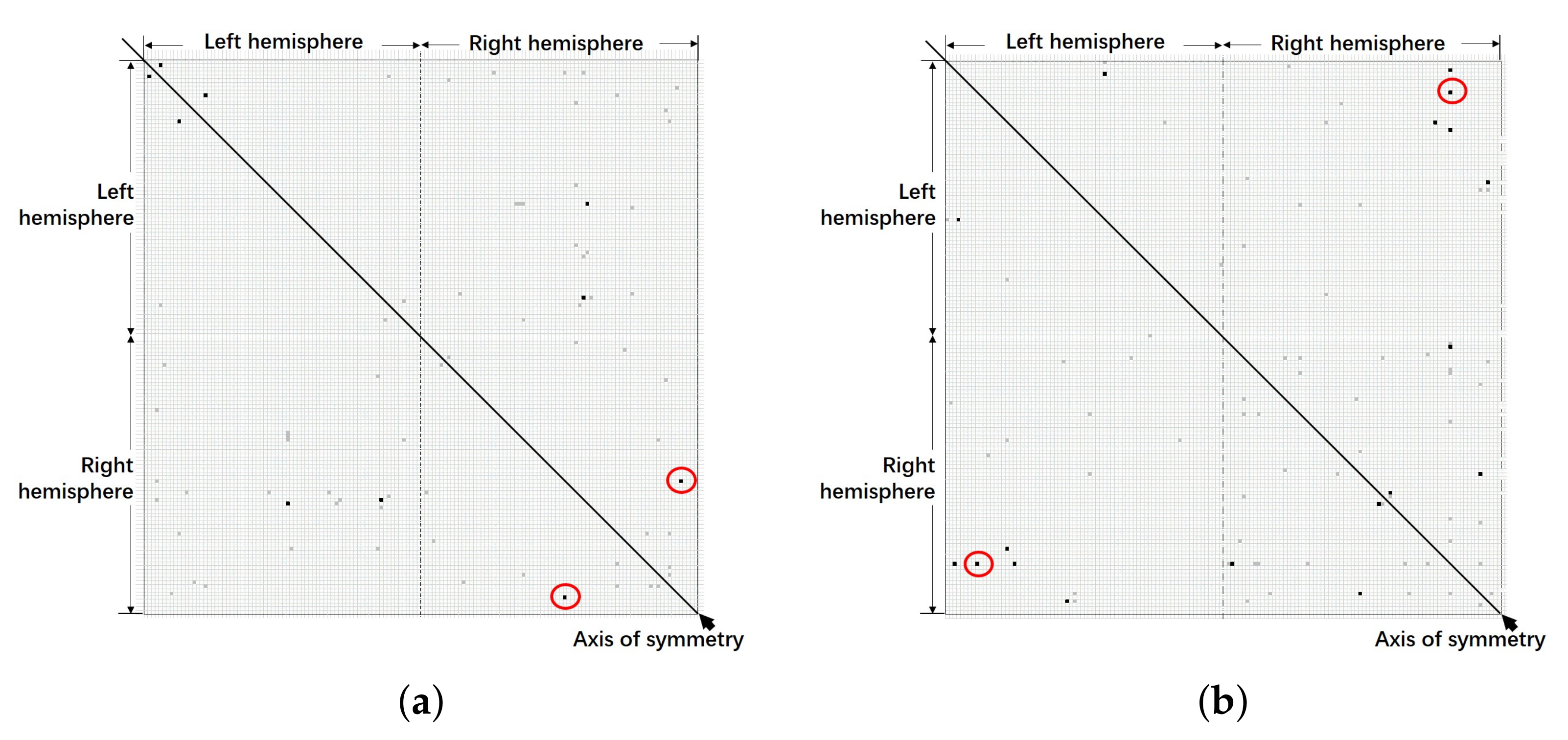
5.1. Lateral and Suborbital Sulcus
5.2. Cingulate Gyrus and Lateral Occipito-Temporal Sulcus
6. Conclusions, Limitations, and Future Research
Supplementary Materials
Author Contributions
Funding
Institutional Review Board Statement
Informed Consent Statement
Data Availability Statement
Acknowledgments
Conflicts of Interest
Appendix A. Some Properties of New Distributions[
Appendix B. The Construction of the N-EM Algorithm
Appendix B.1. ML Estimation of Parameters in the Bivariate NPIG Distribution
Appendix B.2. ML Estimation of Parameters in the Bivariate NPGA Distribution
References
- Ferrari, S.; Cribari-Neto, F. Beta regression for modelling rates and proportions. J. Appl. Stat. 2004, 31, 799–815. [Google Scholar] [CrossRef]
- Simas, A.B.; Barreto-Souza, W.; Rocha, A.V. Improved estimators for a general class of beta regression models. Comput. Stat. Data Anal. 2010, 54, 348–366. [Google Scholar] [CrossRef] [Green Version]
- Ferrari, S.L.P.; Pinheiro, E.C. Improved likelihood inference in beta regression. J. Stat. Comput. Simul. 2011, 81, 431–443. [Google Scholar] [CrossRef]
- Kieschnick, R.; McCullough, B.D. Regression analysis of variates observed on (0, 1): Percentages, proportions and fractions. Stat. Model. 2003, 3, 193–213. [Google Scholar] [CrossRef] [Green Version]
- Zhang, P.; Qiu, Z.G. Regression analysis of proportional data using simplex distribution. Sci. Sin. Math. 2014, 44, 89–104. (In Chinese) [Google Scholar] [CrossRef] [Green Version]
- Lijoi, A.; Mena, R.H.; Prünster, I. Hierarchical mixture modeling with normalized inverse–Gaussian priors. J. Am. Stat. Assoc. 2005, 100, 1278–1291. [Google Scholar] [CrossRef]
- Liu, P.Y.; Tian, G.L.; Yuen, K.C.; Zhang, C.; Tang, M.L. Proportional inverse Gaussian distribution: A new tool for analyzing continuous proportional data. Aust. N. Z. J. Stat. 2021, (in press). [Google Scholar] [CrossRef]
- Wang, C.; Tu, D. A bootstrap semiparametric homogeneity test for the distributions of multigroup proportional data, with applications to analysis of quality of life outcomes in clinical trials. Stat. Med. 2020, 39, 1715–1731. [Google Scholar] [CrossRef]
- Connor, R.J.; Mosimann, J.E. Concepts of independence for proportions with a generalization of the Dirichlet distribution. J. Am. Stat. Assoc. 1969, 64, 194–206. [Google Scholar] [CrossRef]
- Campbell, G.; Mosimann, J.E. Multivariate methods for proportional shape. ASA Proc. Sect. Stat. Graph. 1987, 1, 10–17. [Google Scholar]
- Gueorguieva, R.; Rosenheck, R.; Zelterman, D. Dirichlet component regression and its applications to psychiatric data. Comput. Stat. Data Anal. 2008, 52, 5344–5355. [Google Scholar] [CrossRef] [PubMed] [Green Version]
- Zhang, B. On Compositional Data Modeling and Its Biomedical Applications. Ph.D. Dissertation, Columbia University, New York, NY, USA, 2013. [Google Scholar]
- Morais, J.; Thomas-Agnan, C.; Simioni, M. Using compositional and Dirichlet models for market share regression. J. Appl. Stat. 2018, 45, 1670–1689. [Google Scholar] [CrossRef] [Green Version]
- Cepeda-Cuervo, E.; Achcar, J.A.; Lopera, L.G. Bivariate beta regression models: Joint modeling of the mean, dispersion and association parameters. J. Appl. Stat. 2014, 41, 677–687. [Google Scholar] [CrossRef]
- Petterle, R.R.; Laureano, H.A.; da Silva, G.P.; Bonat, W.H. Multivariate generalized linear mixed models for continuous bounded outcomes: Analyzing the body fat percentage data. Stat. Methods Med. Res. 2021, 30, 2619–2633. [Google Scholar] [CrossRef] [PubMed]
- Sun, Y.; Tian, G.L.; Guo, S.X.; Liu, P.Y. New models for analyzing positively correlated continuous proportional data: A cortical thickness study for schizophrenia. Biometrics 2021. (submitted). [Google Scholar]
- Tweedie, M.C.K. Statistical properties of inverse Gaussian distributions. I. Ann. Math. Stat. 2018, 28, 362–377. [Google Scholar] [CrossRef]
- Palaniyappan, L.; Liddle, P.F. Diagnostic discontinuity in psychosis: A combined study of cortical gyrification and functional connectivity. Schizophr. Bull. 2014, 40, 675–684. [Google Scholar] [CrossRef]
- Destrieux, C.; Fischl, B.; Dale, A.; Halgren, E. Automatic parcellation of human cortical gyri and sulci using standard anatomical nomenclature. NeuroImage 2010, 53, 1–15. [Google Scholar] [CrossRef] [Green Version]
- Fischl, B.; Dale, A.M. Measuring the thickness of the human cerebral cortex from magnetic resonance images. Proc. Natl. Acad. Sci. USA 2000, 97, 11050–11055. [Google Scholar] [CrossRef] [Green Version]
- McLachlan, G.J.; Krishnan, T. The EM Algorithm and Extensions, 2nd ed.; John Wiley & Sons: New York, NY, USA, 2007. [Google Scholar]
- Lange, K. MM Optimization Algorithms; Society for Industrial and Applied Mathematics: Philadelphia, PA, USA, 2016. [Google Scholar]
- Guo, S.X.; Palaniyappan, L.; Liddle, F.P.; Feng, J.F. Dynamic cerebral reorganization in the pathophysiology of schizophrenia: A MRI-derived cortical thickness study. Psychol. Med. 2016, 46, 2201–2214. [Google Scholar]
- Lange, K.; Hunter, D.R.; Yang, I. Optimization transfer using surrogate objective functions (with discussions). J. Comput. Graph. Stat. 2000, 9, 1–20. [Google Scholar]
- Hunter, D.R.; Lange, K. A tutorial on MM algorithms. Am. Stat. 2004, 58, 30–37. [Google Scholar] [CrossRef]
- Tian, G.L.; Huang, X.F.; Xu, J.F. An assembly and decomposition approach for constructing separable minorizing functions in a class of MM algorithms. Stat. Sin. 2004, 29, 961–982. [Google Scholar] [CrossRef] [Green Version]


| ( | |||||||
| Parameter | Ave-MLE | Std | MSE | Ave-MLE | Std | MSE | |
| 1.358641 | 0.442545 | 0.221013 | 1.316643 | 0.362304 | 0.144870 | ||
| 0.298424 | 0.036809 | 0.001357 | 0.298486 | 0.028556 | 0.000818 | ||
| 0.799534 | 0.031722 | 0.001007 | 0.801276 | 0.023760 | 0.000566 | ||
| it.no = 231, = −0.2569 | it.no = 224, = −0.2564 | ||||||
| 1.243133 | 0.237282 | 0.058163 | 1.209933 | 0.121216 | 0.014792 | ||
| 0.300323 | 0.020431 | 0.000418 | 0.300539 | 0.012035 | 0.000145 | ||
| 0.799605 | 0.016497 | 0.000272 | 0.799794 | 0.009520 | 0.000091 | ||
| it.no = 213, = −0.2586 | it.no = 197, = −0.2588 | ||||||
| ( | |||||||
| Parameter | Ave-MLE | Std | MSE | Ave-MLE | Std | MSE | |
| 0.566086 | 0.174171 | 0.034703 | 0.544802 | 0.128736 | 0.018580 | ||
| 0.498231 | 0.048484 | 0.002354 | 0.499272 | 0.037687 | 0.001421 | ||
| 0.601595 | 0.046221 | 0.002139 | 0.600750 | 0.035776 | 0.001280 | ||
| it.no = 172, = −0.4366 | it.no = 167, = −0.4379 | ||||||
| 0.519031 | 0.085486 | 0.007670 | 0.504517 | 0.049257 | 0.002447 | ||
| 0.500203 | 0.026148 | 0.000684 | 0.500225 | 0.015722 | 0.000247 | ||
| 0.600492 | 0.025049 | 0.000628 | 0.599723 | 0.014972 | 0.000224 | ||
| it.no = 157, = −0.4386 | it.no = 145, = −0.4391 | ||||||
| ( | |||||||
| Parameter | Ave-MLE | Std | MSE | Ave-MLE | Std | MSE | |
| 0.220128 | 0.055619 | 0.003499 | 0.211129 | 0.041009 | 0.001806 | ||
| 0.800242 | 0.031396 | 0.000986 | 0.800302 | 0.022899 | 0.000524 | ||
| 0.099971 | 0.018400 | 0.000339 | 0.099890 | 0.013603 | 0.000185 | ||
| it.no = 119, = −0.7350 | it.no = 114, = −0.7338 | ||||||
| 0.205324 | 0.027086 | 0.000762 | 0.201148 | 0.015389 | 0.000238 | ||
| 0.799645 | 0.016570 | 0.000275 | 0.800039 | 0.009393 | 0.000088 | ||
| 0.100182 | 0.009942 | 0.000099 | 0.100087 | 0.005523 | 0.000031 | ||
| it.no = 107, = −0.7326 | it.no = 97, = −0.7323 | ||||||
| Parameter | Ave-MLE | Std | MSE | Ave-MLE | Std | MSE | |
| 0.616064 | 0.098125 | 0.009887 | 0.594675 | 0.054724 | 0.003023 | ||
| 1.197065 | 0.182278 | 0.033234 | 1.202689 | 0.051280 | 0.002637 | ||
| 0.791274 | 0.159555 | 0.025534 | 0.797376 | 0.050753 | 0.002583 | ||
| −0.503090 | 0.172935 | 0.029916 | −0.501269 | 0.052572 | 0.002765 | ||
| 0.496402 | 0.052044 | 0.002721 | 0.495028 | 0.022855 | 0.000547 | ||
| 1.493490 | 0.172693 | 0.029865 | 1.493448 | 0.059934 | 0.003635 | ||
| −1.994148 | 0.159105 | 0.025349 | −1.994163 | 0.055346 | 0.003097 | ||
| 0.693314 | 0.189516 | 0.035961 | 0.695733 | 0.044827 | 0.002028 | ||
| −0.497199 | 0.051602 | 0.002671 | −0.496026 | 0.023453 | 0.000566 | ||
| it.no = 141 | it.no = 68 | ||||||
| 0.594409 | 0.040014 | 0.001632 | 0.592610 | 0.034314 | 0.001232 | ||
| 1.199199 | 0.032275 | 0.001042 | 1.200771 | 0.021140 | 0.000447 | ||
| 0.795187 | 0.036466 | 0.001353 | 0.798587 | 0.025180 | 0.000636 | ||
| −0.500220 | 0.028680 | 0.000823 | −0.500038 | 0.021437 | 0.000460 | ||
| 0.499380 | 0.019778 | 0.000392 | 0.496742 | 0.018138 | 0.000340 | ||
| 1.494840 | 0.035134 | 0.001261 | 1.495448 | 0.025697 | 0.000681 | ||
| −1.997357 | 0.033092 | 0.001102 | −1.997702 | 0.025642 | 0.000663 | ||
| 0.698411 | 0.028526 | 0.000816 | 0.697747 | 0.020047 | 0.000407 | ||
| −0.498473 | 0.019025 | 0.000364 | −0.497432 | 0.015664 | 0.000252 | ||
| it.no = 55 | it.no = 49 | ||||||
| Parameter | Ave-MLE | Std | MSE | Ave-MLE | Std | MSE | |
| 1.997760 | 0.026205 | 0.000692 | 1.998313 | 0.023109 | 0.000537 | ||
| 0.898923 | 0.010484 | 0.000111 | 0.899695 | 0.008393 | 0.000071 | ||
| 0.202299 | 0.019508 | 0.000386 | 0.200620 | 0.015605 | 0.000244 | ||
| it.no = 27, = −0.8064 | it.no = 27, = −0.8078 | ||||||
| 1.999660 | 0.024147 | 0.000583 | 1.998969 | 0.020451 | 0.000419 | ||
| 0.900010 | 0.005360 | 0.000029 | 0.899674 | 0.003072 | 0.000010 | ||
| 0.201871 | 0.010523 | 0.000114 | 0.201171 | 0.006473 | 0.000043 | ||
| it.no = 26, = −0.8072 | it.no = 27, = −0.8074 | ||||||
| Parameter | Ave-MLE | Std | MSE | Ave-MLE | Std | MSE | |
| 5.001001 | 0.036186 | 0.001310 | 4.998937 | 0.032888 | 0.001083 | ||
| 0.402014 | 0.026780 | 0.000721 | 0.402845 | 0.020853 | 0.000443 | ||
| 0.598549 | 0.026008 | 0.000679 | 0.598827 | 0.020339 | 0.000415 | ||
| it.no = 21, = −0.4069 | it.no = 21, = −0.4074 | ||||||
| 4.996352 | 0.042099 | 0.001786 | 5.001158 | 0.038537 | 0.001486 | ||
| 0.400435 | 0.015158 | 0.000230 | 0.399487 | 0.008230 | 0.000068 | ||
| 0.599306 | 0.015034 | 0.000227 | 0.600232 | 0.007946 | 0.000063 | ||
| it.no = 21, = −0.4061 | it.no = 16, = −0.4053 | ||||||
| Parameter | Ave-MLE | Std | MSE | Ave-MLE | Std | MSE | |
| 1.273002 | 0.200704 | 0.045612 | 1.227011 | 0.092474 | 0.009281 | ||
| −0.863261 | 0.274594 | 0.076752 | −0.860950 | 0.137262 | 0.020366 | ||
| 1.374930 | 0.482249 | 0.233192 | 1.341559 | 0.226420 | 0.054681 | ||
| −0.489769 | 0.324336 | 0.105299 | −0.481630 | 0.147419 | 0.022070 | ||
| 0.437918 | 0.290704 | 0.088363 | 0.4730029 | 0.140378 | 0.020435 | ||
| −0.146745 | 0.492742 | 0.245631 | −0.177881 | 0.230247 | 0.053503 | ||
| −0.784241 | 0.340255 | 0.116021 | −0.773613 | 0.157350 | 0.025455 | ||
| it.no = 51 | it.no = 44 | ||||||
| 1.218954 | 0.072089 | 0.005556 | 1.210845 | 0.028854 | 0.000950 | ||
| −0.867234 | 0.106863 | 0.012493 | −0.867112 | 0.042890 | 0.002921 | ||
| 1.362347 | 0.170824 | 0.030598 | 1.353711 | 0.068964 | 0.006899 | ||
| −0.486299 | 0.120704 | 0.014757 | −0.486765 | 0.048496 | 0.002527 | ||
| 0.467544 | 0.101781 | 0.011413 | 0.476607 | 0.042584 | 0.002361 | ||
| −0.168965 | 0.166065 | 0.028541 | −0.174730 | 0.069102 | 0.005414 | ||
| −0.772744 | 0.117103 | 0.014456 | −0.777010 | 0.049669 | 0.002996 | ||
| it.no = 42 | it.no = 36 | ||||||
| Mean1 | Mean2 | Var1 | Var2 | Cov | Coef | |
|---|---|---|---|---|---|---|
| 0.2 | 0.5 | 0.6 | 0.095957 | 0.095424 | −0.041228 | −0.430854 |
| 0.4 | 0.5 | 0.6 | 0.080300 | 0.081386 | −0.035332 | −0.437049 |
| 0.6 | 0.5 | 0.6 | 0.069668 | 0.071562 | −0.031100 | −0.440454 |
| 0.8 | 0.5 | 0.6 | 0.061796 | 0.064130 | −0.027863 | −0.442600 |
| 1 | 0.5 | 0.6 | 0.055664 | 0.058245 | −0.025285 | −0.444056 |
| 3 | 0.5 | 0.6 | 0.028704 | 0.031267 | −0.013426 | −0.448160 |
| 5 | 0.5 | 0.6 | 0.019542 | 0.021624 | −0.009222 | −0.448594 |
| 10 | 0.5 | 0.6 | 0.010927 | 0.012291 | −0.005197 | −0.448441 |
| 15 | 0.5 | 0.6 | 0.007596 | 0.008602 | −0.003623 | −0.448208 |
| 20 | 0.5 | 0.6 | 0.005823 | 0.006620 | −0.002782 | −0.448038 |
| 0.2 | 0.3 | 0.8 | 0.085745 | 0.066704 | −0.019270 | −0.254800 |
| 0.4 | 0.3 | 0.8 | 0.074236 | 0.058458 | −0.016938 | −0.257123 |
| 0.6 | 0.3 | 0.8 | 0.065981 | 0.052423 | −0.015181 | −0.258120 |
| 0.8 | 0.3 | 0.8 | 0.059627 | 0.047708 | −0.013789 | −0.258536 |
| 1 | 0.3 | 0.8 | 0.054527 | 0.043879 | −0.012652 | −0.258650 |
| 3 | 0.3 | 0.8 | 0.030294 | 0.025118 | −0.007072 | −0.256390 |
| 5 | 0.3 | 0.8 | 0.021249 | 0.017844 | −0.004950 | −0.254195 |
| 10 | 0.3 | 0.8 | 0.012261 | 0.010441 | −0.002841 | −0.251100 |
| 15 | 0.3 | 0.8 | 0.008637 | 0.007400 | −0.001995 | −0.249545 |
| 20 | 0.3 | 0.8 | 0.006671 | 0.005735 | −0.001538 | −0.248617 |
| 0.2 | 0.8 | 0.1 | 0.047708 | 0.020039 | −0.022637 | −0.732127 |
| 0.4 | 0.8 | 0.1 | 0.035625 | 0.013569 | −0.016702 | −0.759669 |
| 0.6 | 0.8 | 0.1 | 0.028700 | 0.010334 | −0.013357 | −0.775590 |
| 0.8 | 0.8 | 0.1 | 0.024122 | 0.008365 | −0.011170 | −0.786306 |
| 1 | 0.8 | 0.1 | 0.020844 | 0.007035 | −0.009616 | −0.794114 |
| 3 | 0.8 | 0.1 | 0.008965 | 0.002734 | −0.004079 | −0.823825 |
| 5 | 0.8 | 0.1 | 0.005735 | 0.001700 | −0.002599 | −0.832436 |
| 10 | 0.8 | 0.1 | 0.003022 | 0.000874 | −0.001365 | −0.839907 |
| 15 | 0.8 | 0.1 | 0.002052 | 0.000588 | −0.000926 | −0.842639 |
| 20 | 0.8 | 0.1 | 0.001554 | 0.000443 | −0.000701 | −0.844056 |
| Mean1 | Mean2 | Var1 | Var2 | Cov | Coef | |
|---|---|---|---|---|---|---|
| 0.2 | 0.9 | 0.2 | 0.030000 | 0.080000 | −0.031973 | −0.652641 |
| 0.4 | 0.9 | 0.2 | 0.018000 | 0.053333 | −0.022113 | −0.713705 |
| 0.6 | 0.9 | 0.2 | 0.012857 | 0.040000 | −0.016892 | −0.744877 |
| 0.8 | 0.9 | 0.2 | 0.010000 | 0.032000 | −0.013669 | −0.764106 |
| 1 | 0.9 | 0.2 | 0.008182 | 0.026667 | −0.011480 | −0.777230 |
| 3 | 0.9 | 0.2 | 0.002903 | 0.010000 | −0.004421 | −0.820416 |
| 5 | 0.9 | 0.2 | 0.001765 | 0.006154 | −0.002738 | −0.830996 |
| 10 | 0.9 | 0.2 | 0.000891 | 0.003137 | −0.001404 | −0.839489 |
| 15 | 0.9 | 0.2 | 0.000596 | 0.002105 | −0.000944 | −0.842438 |
| 20 | 0.9 | 0.2 | 0.000448 | 0.001584 | −0.000711 | −0.843936 |
| 0.2 | 0.4 | 0.7 | 0.180000 | 0.163333 | −0.052559 | −0.306532 |
| 0.4 | 0.4 | 0.7 | 0.144000 | 0.133636 | −0.045743 | −0.329747 |
| 0.6 | 0.4 | 0.7 | 0.120000 | 0.113077 | −0.039804 | −0.341705 |
| 0.8 | 0.4 | 0.7 | 0.102857 | 0.098000 | −0.034977 | −0.348383 |
| 1 | 0.4 | 0.7 | 0.090000 | 0.086471 | −0.031078 | −0.352290 |
| 3 | 0.4 | 0.7 | 0.040000 | 0.039730 | −0.014237 | −0.357122 |
| 5 | 0.4 | 0.7 | 0.025714 | 0.025789 | −0.009141 | −0.354974 |
| 10 | 0.4 | 0.7 | 0.013585 | 0.013738 | −0.004805 | −0.351719 |
| 15 | 0.4 | 0.7 | 0.009231 | 0.009363 | −0.003256 | −0.350212 |
| 20 | 0.4 | 0.7 | 0.006990 | 0.007101 | −0.002462 | −0.349366 |
| 0.2 | 0.2 | 0.2 | 0.128000 | 0.080000 | −0.026476 | −0.261637 |
| 0.4 | 0.2 | 0.2 | 0.106667 | 0.053333 | −0.022288 | −0.295506 |
| 0.6 | 0.2 | 0.2 | 0.091429 | 0.040000 | −0.019121 | −0.316183 |
| 0.8 | 0.2 | 0.2 | 0.080000 | 0.032000 | −0.016708 | −0.330219 |
| 1 | 0.2 | 0.2 | 0.071111 | 0.026667 | −0.014822 | −0.340368 |
| 3 | 0.2 | 0.2 | 0.033684 | 0.010000 | −0.006910 | −0.376481 |
| 5 | 0.2 | 0.2 | 0.022069 | 0.006154 | −0.004494 | −0.385587 |
| 10 | 0.2 | 0.2 | 0.011852 | 0.003137 | −0.002395 | −0.392746 |
| 15 | 0.2 | 0.2 | 0.008101 | 0.002105 | −0.001632 | −0.395167 |
| 20 | 0.2 | 0.2 | 0.006154 | 0.001584 | −0.001238 | −0.396378 |
| Par. | Controls | Patients | ||||
|---|---|---|---|---|---|---|
| MLE | CI | Std | MLE | CI | Std | |
| Bivariate PIG distribution | Bivariate NPIG distribution | |||||
| 0.4296 | [0.2744, 0.7503] | 0.1242 | 0.4837 | [0.3158, 0.8444] | 0.1370 | |
| 0.4664 | [0.3821, 0.5473] | 0.0416 | 0.4249 | [0.3504, 0.5042] | 0.0399 | |
| 0.5029 | [0.4213, 0.5877] | 0.0427 | 0.4209 | [0.3438, 0.4923] | 0.0378 | |
| AIC = 18.0480; BIC = 23.1147 | AIC = 1.4008; BIC = 6.5415 | |||||
| Bivariate PGA distribution | Bivariate NPGA distribution | |||||
| 1.4540 | [1.0527, 2.0820] | 0.2606 | 1.5477 | [1.2360, 1.8403] | 0.1418 | |
| 0.5071 | [0.4317, 0.5812] | 0.0373 | 0.4294 | [0.3659, 0.5023] | 0.0359 | |
| 0.5161 | [0.4454, 0.5881] | 0.0383 | 0.4059 | [0.3394, 0.4676] | 0.0319 | |
| AIC = 2.0847; BIC = 7.1514 | AIC = −9.9734; BIC = −4.8327 | |||||
| Par. | Controls | Patients | ||||
|---|---|---|---|---|---|---|
| MLE | CI | Std | MLE | CI | Std | |
| Bivariate PIG mean regression | Bivariate NPIG mean regression | |||||
| 0.5588 | [0.3899, 1.0599] | 0.1789 | 0.5355 | [0.4019, 1.0499] | 0.1579 | |
| 4.9412 | [1.7141, 8.1186] | 1.6109 | 2.6217 | [−1.0682, 6.7279] | 1.8809 | |
| −1.5045 | [−2.4762, −0.6009] | 0.4686 | −0.8339 | [−2.0480, 0.2186] | 0.5428 | |
| 0.6536 | [0.0220, 1.4045] | 0.3506 | −0.0466 | [−0.7188, 0.7475] | 0.3654 | |
| 4.0251 | [0.7731, 7.6577] | 1.6832 | 0.4262 | [−3.5984, 4.4486] | 1.8909 | |
| −1.1637 | [−2.2148, −0.2369] | 0.4891 | −0.2414 | [−1.3743, 0.8807] | 0.5476 | |
| 0.1555 | [−0.4933, 0.8664] | 0.3469 | 0.3114 | [−0.5136, 0.9808] | 0.3816 | |
| AIC = 15.0705; BIC = 26.8926 | AIC = 4.6480; BIC = 16.6430 | |||||
| Bivariate PGA mean regression | Bivariate NPGA mean regression | |||||
| 1.5535 | [1.1976, 2.2985] | 0.2744 | 1.6295 | [1.2301, 2.5405] | 0.3288 | |
| 6.1568 | [4.3330, 7.6466] | 0.7389 | 1.4482 | [−1.7922, 5.0879] | 1.7278 | |
| −1.7962 | [−2.2712, −1.2685] | 0.2251 | −0.4871 | [−1.5415, 0.4178] | 0.4990 | |
| 0.4822 | [0.0032, 1.0710] | 0.2857 | −0.1693 | [−0.7979, 0.4999] | 0.3374 | |
| 4.8569 | [3.3534, 6.5856] | 0.7110 | 1.8815 | [−1.3326, 4.7364] | 1.5787 | |
| −1.3976 | [−1.9201, −0.9069] | 0.2127 | −0.6746 | [−1.5283, 0.2427] | 0.4539 | |
| 0.2720 | [−0.2365, 0.9072] | 0.2990 | 0.3070 | [−0.2977, 0.8459] | 0.3052 | |
| AIC = 4.2536; BIC = 16.0757 | AIC = −6.7527; BIC = 5.2424 | |||||
| Par. | Patients | Controls | ||||
|---|---|---|---|---|---|---|
| MLE | CI | Std | MLE | CI | Std | |
| Bivariate PIG distribution | Bivariate NPIG distribution | |||||
| 0.6307 | [0.4001, 1.1844] | 0.1903 | 1.6761 | [1.1946, 2.6281] | 0.3711 | |
| 0.4010 | [0.3243, 0.4790] | 0.0396 | 0.5031 | [0.4390, 0.5676] | 0.0325 | |
| 0.4552 | [0.3859, 0.5331] | 0.0386 | 0.5215 | [0.4614, 0.5843] | 0.0320 | |
| AIC = 4.1243; BIC = 9.2650 | AIC = −29.0117; BIC = −23.9451 | |||||
| Bivariate PGA distribution | Bivariate NPGA distribution | |||||
| 1.9787 | [1.5283, 2.8760] | 0.3586 | 3.0165 | [2.8431, 3.1387] | 0.0711 | |
| 0.3967 | [0.3249, 0.4524] | 0.0334 | 0.5000 | [0.4531, 0.5639] | 0.0267 | |
| 0.4650 | [0.4009, 0.5221] | 0.0334 | 0.5374 | [0.4771, 0.5886] | 0.0273 | |
| AIC = −12.8517; BIC = −7.7109 | AIC = −43.0450; BIC = −37.9783 | |||||
| Par. | Patients | Controls | ||||
|---|---|---|---|---|---|---|
| MLE | CI | Std | MLE | CI | Std | |
| Bivariate PIG mean regression | Bivariate NPIG mean regression | |||||
| 0.7825 | [0.5220, 1.3723] | 0.2194 | 1.8085 | [1.3285, 2.8110] | 0.3876 | |
| 3.4074 | [0.3196, 6.1716] | 1.5023 | 3.2295 | [0.3851, 6.4295] | 1.5459 | |
| −1.0921 | [−1.9158, −0.2041] | 0.4349 | −0.9194 | [−1.8404, −0.0923] | 0.4459 | |
| 3.6225 | [0.4132, 6.5227] | 1.5104 | −0.1836 | [−2.8446, 2.9085] | 1.4255 | |
| −1.0925 | [−1.9570, −0.1878] | 0.4373 | 0.0806 | [−0.8328, 0.8209] | 0.4091 | |
| AIC = 0.0722; BIC = 8.6400 | AIC = −31.1357; BIC = −22.6913 | |||||
| Bivariate PGA mean regression | Bivariate NPGA mean regression | |||||
| 2.1331 | [1.6301, 3.0572] | 0.3632 | 3.2817 | [2.5071, 4.8420] | 0.6160 | |
| 3.0007 | [1.0820, 4.6351] | 0.7655 | 3.2619 | [0.4007, 6.0649] | 1.4288 | |
| −0.9823 | [−1.4382, −0.4542] | 0.2243 | −0.9366 | [−1.7524, −0.1013] | 0.4134 | |
| 2.6646 | [0.8734, 4.2967] | 0.8151 | −0.0168 | [−2.9359, 2.9117] | 1.5148 | |
| −0.8051 | [−1.3183, −0.3098] | 0.2397 | 0.0486 | [−0.8062, 0.8667] | 0.4337 | |
| AIC = −16.1259; BIC = −7.5581 | AIC = −46.5825; BIC = −38.1381 | |||||
Publisher’s Note: MDPI stays neutral with regard to jurisdictional claims in published maps and institutional affiliations. |
© 2022 by the authors. Licensee MDPI, Basel, Switzerland. This article is an open access article distributed under the terms and conditions of the Creative Commons Attribution (CC BY) license (https://creativecommons.org/licenses/by/4.0/).
Share and Cite
Sun, Y.; Tian, G.; Guo, S.; Shu, L.; Zhang, C. Bivariate Continuous Negatively Correlated Proportional Models with Applications in Schizophrenia Research. Mathematics 2022, 10, 353. https://doi.org/10.3390/math10030353
Sun Y, Tian G, Guo S, Shu L, Zhang C. Bivariate Continuous Negatively Correlated Proportional Models with Applications in Schizophrenia Research. Mathematics. 2022; 10(3):353. https://doi.org/10.3390/math10030353
Chicago/Turabian StyleSun, Yuan, Guoliang Tian, Shuixia Guo, Lianjie Shu, and Chi Zhang. 2022. "Bivariate Continuous Negatively Correlated Proportional Models with Applications in Schizophrenia Research" Mathematics 10, no. 3: 353. https://doi.org/10.3390/math10030353
APA StyleSun, Y., Tian, G., Guo, S., Shu, L., & Zhang, C. (2022). Bivariate Continuous Negatively Correlated Proportional Models with Applications in Schizophrenia Research. Mathematics, 10(3), 353. https://doi.org/10.3390/math10030353