Bivariate Continuous Negatively Correlated Proportional Models with Applications in Schizophrenia Research

Abstract

Bivariate continuous negatively correlated proportional data defined in the unit square ${(0,1)}^2$ often appear in many different disciplines, such as medical studies, clinical trials and so on. To model this type of data, the paper proposes two new bivariate continuous distributions (i.e., negatively correlated proportional inverse Gaussian (NPIG) and negatively correlated proportional gamma (NPGA) distributions) for the first time and provides corresponding distributional properties. Two mean regression models are further developed for data with covariates. The normalized expectation–maximization (N-EM) algorithm and the gradient descent algorithm are combined to obtain the maximum likelihood estimates of parameters of interest. Simulations studies are conducted, and a data set of cortical thickness for schizophrenia is used to illustrate the proposed methods. According to our analysis between patients and controls of cortical thickness in typical mutual inhibitory brain regions, we verified the compensatory of cortical thickness in patients with schizophrenia and found its negative correlation with age.

1. Introduction

In many aspects, experimental results or measurements are reported in the form of ratios, scores, proportions or percentages, which is frequently encountered in sociology, psychology, epidemiology and clinical trials. The characteristic of the data is that they are continuously valued within the unit interval $(0,1)$; thus, models focusing on this limited range are worthwhile. Researchers have developed different strategies for modeling such kinds of data. First, the beta distribution and beta regression models have been exhaustively studied by many authors, including [1,2,3]. Kieschnick and McCullough [4] summarized and compared different regression models for proportional data in the open interval. Next, the simplex distribution investigated by Zhang and Qiu [5] can also be utilized to model such continuous proportional data, and they further pointed out the simplex regression model is more robust than the beta model. By mimicking the construction of beta distributions with gamma variates, Lijoiu et al. [6] proposed a so-called normalized inverse Gaussian (IG) distribution by substituting the gamma variates with IG variates, as a new tool for modeling univariate proportional data. Later, Liu et al. [7] renamed it as the proportional inverse Gaussian (PIG) distribution and set up regression models. Due to the diversity and dimension enlarger of data, we need to generalize the univariate continuous proportional models to multivariate cases. Wang and Tu [8] considered the semiparametric tests for multigroup proportional data in a closed interval $[0,1]$.

From the perspective of data structure, the multi-dimensional data limited in unit intervals can be divided into compositional data and multivariate proportional data according to their domains. For compositional data, which often appear in various fields, such as biology, medicine and economics, the summation of all components of data values equals one, also known as structure relative numbers reflecting the composition of objects. Thus, the corresponding models fitting for the compositional data are defined in the open hyperplane ${\mathbb{T}}_m=\left\{\mathit{x}={(x_1,\cdots ,x_m)}^{\top }:x_j>0,j=1,\cdots ,m,{\mathbf{1}\mathbf{1}}_m^{\top }\mathit{x}=1\right\}$. Due to the constraint of ${\mathbf{1}\mathbf{1}}_m^{\top }\mathit{x}=1$, it leads to certain negative correlations between any two dimensions of compositional data. One of the well-known distributions is the Dirichlet distribution, which can be regarded as a generalization of the beta distribution to more than two components. It was first used to fit two compositional biological data in [9]. Campbell and Mosimann [10] considered a Dirichlet regression model by linking the parameters to a set of covariates via a polynomial function, and the models with applications to the analysis of psychiatric data are investigated in [11]. By the way, the beta distribution could be regarded as a two-dimensional Dirichlet distribution, and a beta variate X and its complement $1-X$ are also negatively correlated. Other research on related models can be found in recent literature [12,13].

For multivariate proportional data, it appears that each component of the data is valued between 0 and 1 with no direct constraint among components. The corresponding models for this type of data are defined in the unit cubic ${(0,1)}^m=\left\{\mathit{x}={(x_1,\cdots ,x_m)}^{\top }:0<x_j<1,j=1,\cdots ,m\right\}$ without restriction ${\mathbf{1}\mathbf{1}}_m^{\top }\mathit{x}=1$. There are many ways to construct appropriate models, such as beta distribution with copula linking functions. Cepeda-Cuervo et al. [14] defined a bivariate beta regression model from copulas and considered the Bayesian approach, in which the correlation could be positive or negative. Petterle et al. [15] proposed a multivariate generalized linear mixed model for modeling continuous bounded variables in the interval $(0,1)$. Sun et al. [16] proposed a linear stochastic representation (SR) to construct multivariate positively correlated continuous models based on IG and gamma distributions, named as multivariate PIG and proportional gamma (PGA) distributions, respectively, which can only fit positively correlated continuous proportional data.

The cortical thickness of schizophrenia data used in [16] shows high correlations and compensation behaviors related to disease severity among different brain regions. Further, we find that a large number of negative covariant region pairs may occur in patients if the changes of compensations are reduced. This indicates the observations of negatively correlated regions in cortical thickness are of great significance for the study of schizophrenia and its prognosis. Motivated by the construction technique in multivariate PIG and PGA distributions, we will propose models to capture the negative correlation among components for multivariate proportional data. To the best of our knowledge, work considering the negative correlation of multivariate proportion data is quite scarce. Here, we focus on the bivariate situations; thus, the proposed models are expected to provide efficient tools in modeling negatively correlated proportional data.

By combining the construction of multivariate PIG/PGA distributions and the negative correlation structure in beta/Dirichlet distributions, we define a new random vector $\mathbf{x}={(X_1,X_2)}^{\top }\in {(0,1)}^2$ via the following SR:

$$X_1=\frac{Y_1}{Y_0+Y_1}\mathrm{and}{X}_2=1-\frac{Y_2}{Y_0+Y_2}=\frac{Y_0}{Y_0+Y_2},$$

(1)

where ${\left\{Y_j\right\}}_{j=0}^2$ are independent random variables with the same support ${\mathbb{R}}_{+}$, and each $Y_j$ can follow any same continuous distribution family but with possibly different parameters. In the following, for each $Y_j$ ($j=0,1,2$), we applied the IG and gamma distributions to construct bivariate negatively correlated PIG (NPIG) and negatively correlated proportional gamma (NPGA) distributions.

The rest of the paper is organized as follows. In Section 2 and Section 3, the bivariate NPIG and NPGA distributions are, respectively, proposed and related distributional properties (e.g., moments, joint densities) are provided. Moreover, the normalized expectation–maximization (N-EM) facilitated by the one-step gradient descent algorithms are established for calculating the maximum likelihood (ML) estimations of parameters of interest. In Section 4, simulations for the proposed methods are performed. A data set on the cortical thickness of schizophrenia is used to illustrate the proposed methods in Section 5. Finally, a discussion is provided in Section 6. Some technical details are put in the Appendix A and Appendix B, and others are shown in the Supplementary Material.

2. Bivariate Negatively Correlated PIG Models

First, we propose a new bivariate NPIG distribution based on equi-dispersed IG distributions and develop the corresponding NPIG mean regression model. The N-EM algorithms for calculating the ML estimators of parameters are also provided.

2.1. Bivariate NPIG Distribution

The IG distribution with location parameter $a$ (>0) and shape parameter $b$ (>0), denoted by $Y\sim \mathrm{IG}(a,b)$, if it has the probability density function (pdf)

$$f_{{}_{IG}}\left(y\right|a,b)=\sqrt{\frac{b}{2\pi }}{y}^{-\frac{3}{2}}exp\left[-\frac{b{(y-a)}^2}{2a^{2}y}\right],y>0.$$

According to the results of [17], we have $E\left(Y\right)=a$ and $\mathrm{Var}\left(Y\right)=a^3/b$. By setting $b=a^2$, the general IG distribution reduces to the equi-dispersed $\mathrm{IG}(a,a^2)$ as its mean equals the variance.

By adopting three independent equi-dispersed IG variates $Y_j\stackrel{\mathrm{ind}}{\sim }\mathrm{IG}({\mu }_j,{\mu }_j^2)$ with ${\mu }_j>0$ for $j=0,1,2$, the random vector defined by (1) is said to follow a bivariate NPIG distribution, denoted by $\mathbf{x}={(X_1,X_2)}^{\top }\sim {\mathrm{NPIG}}_2\left(\mathbf{\mu }\right)$ with $\mathbf{\mu }={({\mu }_0,{\mu }_1,{\mu }_2)}^{\top }$. Since the moment generating functions (MGF) of $Y_j$ is $M_{Y_j}\left(t\right)=exp\left[{\mu }_j(1-\sqrt{1-2t})\right]$, the expectations, variances and the covariance are computed based on (A1)–(A5) as

$$\begin{array}{ccc}\hfill E\left(X_1\right)& =& \frac{{\mu }_1}{{\mu }_0+{\mu }_1}\triangleq {\theta }_1\in (0,1),\hfill \end{array}$$

(2)

$$\begin{array}{ccc}\hfill E\left(X_2\right)& =& \frac{{\mu }_0}{{\mu }_0+{\mu }_2}\triangleq {\theta }_2\in (0,1),\hfill \end{array}$$

(3)

$$\begin{array}{ccc}\hfill \mathrm{Var}\left(X_j\right)& =& {\mu }_0{\mu }_j{\mathrm{e}}^{{\mu }_0+{\mu }_j}\mathrm{\Gamma }(-2,{\mu }_0+{\mu }_j),j=1,2,\hfill \end{array}$$

$$\begin{array}{ccc}\hfill \mathrm{Cov}(X_1,X_2)& =& -{\mu }_1{\mu }_2{\mathrm{e}}^{{\mu }_0+{\mu }_1+{\mu }_2}{\int }_1^{\infty }{\int }_1^{\infty }{\mathrm{e}}^{-{\mu }_{1}t}{\mathrm{e}}^{-{\mu }_{2}s}\left[{\mathrm{e}}^{-{\mu }_0\sqrt{t^2+s^2-1}}-{\mathrm{e}}^{-{\mu }_0(t+s-1)}\right]\mathrm{d}t\mathrm{d}s,\hfill \end{array}$$

where $\mathrm{\Gamma }(-2,{\mu }_0+{\mu }_j)={\int }_{{\mu }_0+{\mu }_j}^{\infty }{t}^{-3}{\mathrm{e}}^{-t}\mathrm{d}t$ is the incomplete gamma function. According to the numerical experiments in [16], the correlation coefficient is limited in the open interval $(-1,0)$. The joint pdf of the bivariate NPIG distribution is derived as

$$f_{{}_{{\mathrm{NPIG}}_2}}\left(\mathit{x}\right|\mathbf{\mu })=\frac{{\prod }_{j=0}^2{\mu }_{j}exp\left({\mu }_j\right)}{{\left(2\pi \right)}^{\frac{3}{2}}{\left[x_1^3{x}_2{(1-x_2)}^3(1-x_1)\right]}^{\frac{1}{2}}}{\int }_0^{\infty }h\left(s\right|\mathit{x},\mathit{\mu })\mathrm{d}s,\mathit{x}={(x_1,x_2)}^{\top }\in {(0,1)}^2,$$

where

$$\begin{array}{ccc}& & h\left(s\right|\mathit{x},\mathit{\mu })=s^{-\frac{5}{2}}exp\left\{-\frac{1}{2}\left[s·a\left(\mathit{x}\right)+\frac{1}{s}·b(\mathit{x},\mathit{\mu })\right]\right\},\hfill \\ & & a\left(\mathit{x}\right)=1+\frac{x_1}{1-x_1}+\frac{1-x_2}{x_2}\mathrm{and}b(\mathit{x},\mathit{\mu })={\mu }_0^2+\frac{1-x_1}{x_1}{\mu }_1^2+\frac{x_2}{1-x_2}{\mu }_2^2.\hfill \end{array}$$

From the perspective of practice, usually, we would like to have intuitive interpretations of population means. Therefore, we re-parametrize the bivariate NPIG distribution in terms of the parameter vector $\mathit{\theta }={({\theta }_0,{\theta }_1,{\theta }_2)}^{\top }$ according to (2) and (3) by making the following one-to-one mapping

$${\mu }_0={\theta }_0,{\mu }_1={\theta }_0{\theta }_1/(1-{\theta }_1)\mathrm{and}{\mu }_2={\theta }_0/{\theta }_2-{\theta }_0.$$

The pdf of the re-parameterized bivariate NPIG distribution, denoted by $\mathbf{x}\sim {\mathrm{NPIG}}_2\left(\mathit{\theta }\right)$, is

$$f_{{}_{{\mathrm{NPIG}}_2}}\left(\mathit{x}\right|\mathit{\theta })=\frac{{\theta }_0^3·\frac{{\theta }_1}{1-{\theta }_1}·\frac{1-{\theta }_2}{{\theta }_2}exp\left({\theta }_0+{\theta }_0·\frac{{\theta }_1}{1-{\theta }_1}+{\theta }_0·\frac{1-{\theta }_2}{{\theta }_2}\right)}{{\left(2\pi \right)}^{\frac{3}{2}}{\left[x_1^3{x}_2{(1-x_2)}^3(1-x_1)\right]}^{\frac{1}{2}}}{\int }_0^{\infty }{h}_1\left(s\right|\mathit{x},\mathit{\theta })\mathrm{d}s,$$

where $\mathit{x}\in {(0,1)}^2$,

$$\begin{array}{ccc}\hfill h_1\left(s\right|\mathit{x},\mathit{\theta })& =& s^{-\frac{5}{2}}exp\left\{-\frac{1}{2}\left[s·a\left(\mathit{x}\right)+\frac{1}{s}·b_1(\mathit{x},\mathit{\theta })\right]\right\}\mathrm{and}\hfill \end{array}$$

$$\begin{array}{ccc}\hfill b_1(\mathit{x},\mathit{\theta })& =& {\theta }_0^2\left[1+\frac{(1-x_1){\theta }_1^2}{x_1{(1-{\theta }_1)}^2}+\frac{x_2{(1-{\theta }_2)}^2}{(1-x_2){\theta }_2^2}\right].\hfill \end{array}$$

(4)

Figure 1 plots the bivariate NPIG distribution ${\mathrm{NPIG}}_2\left(\mathit{\theta }\right)$ with two sets of different values of parameters. We note that a larger value of ${\theta }_0$ makes the distribution more concentrated, and it also influences the number of modes. When ${\theta }_0$ is large enough, the change in the values of ${({\theta }_1,{\theta }_2)}^{\top }$ affects the location of modes and the skewness of distributions. Thus, it is appropriate to regard ${\theta }_0$ as the dispersion parameter and ${\theta }_1,{\theta }_2$ as the two location parameters. Sometimes, while the distributions are dense and unimodal, the modes are very different from the expectations.

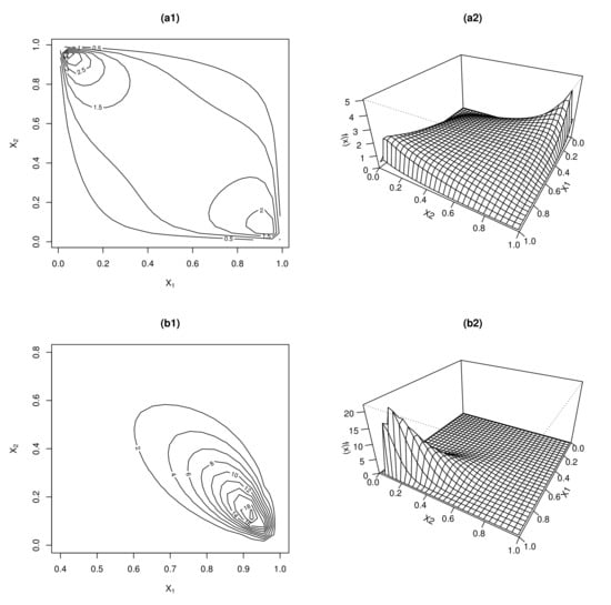
Figure 1. The contour plots and 3D perspectives of the bivariate NPIG distribution ${\mathrm{NPIG}}_2\left(\mathit{\theta }\right)$ with different values of parameters: (a1,a2) $\mathit{\theta }={(0.5,0.5,0.5)}^{\top }$; (b1,b2) $\mathit{\theta }={(1.5,0.8,0.3)}^{\top }$.

2.2. ML Estimation of Parameters via the N-EM Algorithm

Let ${\mathbf{x}}_1,\dots ,{\mathbf{x}}_n\stackrel{\mathrm{iid}}{\sim }{\mathrm{NPIG}}_2\left(\mathit{\theta }\right)$ and $Y_{{\mathrm{obs}}_1}={\left\{{\mathit{x}}_i\right\}}_{i=1}^n$ denote the observed data, where ${\mathit{x}}_i={(x_{i1},x_{i2})}^{\top }$ is the realization of ${\mathbf{x}}_i={(X_{i1},X_{i2})}^{\top }$. The log-likelihood function of the parameter vector $\mathit{\theta }$ is given by

$$\begin{array}{ccc}\hfill {\ell }_1\left(\mathit{\theta }\right|Y_{{\mathrm{obs}}_1})& =& 3nlog{\theta }_0+n{\theta }_0+n\frac{{\theta }_0{\theta }_1}{1-{\theta }_1}+nlog\frac{{\theta }_1}{1-{\theta }_1}+n\frac{{\theta }_0(1-{\theta }_2)}{{\theta }_2}+nlog\frac{1-{\theta }_2}{{\theta }_2}\hfill \end{array}$$

$$\begin{array}{ccc}& & +\sum _{i=1}^{n}log\left[{\int }_0^{\infty }{h}_1\left(s\right|{\mathit{x}}_i,\mathit{\theta })\mathrm{d}s\right]+c_1,\hfill \end{array}$$

(5)

where $c_1$ is a constant free from the parameter vector $\mathit{\theta }$. Due to the existence of the intractable integrals in (5), neither the Newton–Raphson nor the Fisher scoring algorithm is attainable in dealing with the above expression. Instead, we adopt the N-EM algorithm, which is composed of three steps:

N-step:

Establish the following normalized density function based on $h_1(·|{\mathit{x}}_i,\mathit{\theta })$ as

$$g_1\left(s\right|{\mathit{x}}_i,\mathit{\theta })\triangleq \frac{h_1\left(s\right|{\mathit{x}}_i,\mathit{\theta })}{{\int }_0^{\infty }{h}_1\left(t\right|{\mathit{x}}_i,\mathit{\theta })\mathrm{d}t},s>0,$$

so that $g_1\left(s\right|{\mathit{x}}_i,{\mathit{\theta }}^{\left(t\right)})$ is also a valid pdf defined on $(0,\infty )$, where ${\mathit{\theta }}^{\left(t\right)}$ denotes the t-th approximation of $\widehat{\mathit{\theta }}$.

E-step:

Construct a surrogate Q-function by utilizing the integral version of Jensen’s inequality as

$$\begin{array}{ccc}\hfill Q_1\left(\mathit{\theta }\right|{\mathit{\theta }}^{\left(t\right)})& =& 3nlog{\theta }_0+n{\theta }_0+n\frac{{\theta }_0{\theta }_1}{1-{\theta }_1}+nlog\frac{{\theta }_1}{1-{\theta }_1}+n\frac{{\theta }_0(1-{\theta }_2)}{{\theta }_2}\hfill \end{array}$$

$$\begin{array}{ccc}& & +nlog\frac{1-{\theta }_2}{{\theta }_2}-\frac{1}{2}\sum _{i=1}^n\left[B_1({\mathit{x}}_i,{\mathit{\theta }}^{\left(t\right)})·b_1({\mathit{x}}_i,\mathit{\theta })\right]+c_1^{\left(t\right)},\hfill \end{array}$$

(6)

where

$$B_1({\mathit{x}}_i,{\mathit{\theta }}^{\left(t\right)})\triangleq {\int }_0^{\infty }{s}^{-1}·g_1\left(s\right|{\mathit{x}}_i,{\mathit{\theta }}^{\left(t\right)})\mathrm{d}s,$$

$b_1(\mathit{x},\mathit{\theta })$ is defined by (4), and $c_1^{\left(t\right)}$ is a constant not depending on $\mathit{\theta }$. It can be proven that $Q_1\left(\mathit{\theta }\right|{\mathit{\theta }}^{\left(t\right)})$ satisfies

$$Q_1\left(\mathit{\theta }\right|{\mathit{\theta }}^{\left(t\right)})⩽{\ell }_1\left(\mathit{\theta }\right|Y_{{\mathrm{obs}}_1})\mathrm{and}{Q}_1\left({\mathit{\theta }}^{\left(t\right)}\right|{\mathit{\theta }}^{\left(t\right)})={\ell }_1\left({\mathit{\theta }}^{\left(t\right)}\right|Y_{{\mathrm{obs}}_1}),$$

indicating that it minorizes ${\ell }_1\left(\mathit{\theta }\right|Y_{{\mathrm{obs}}_1})$ at $\mathit{\theta }={\mathit{\theta }}^{\left(t\right)}$.

M-step:

Maximize $Q_1\left(\mathit{\theta }\right|{\mathit{\theta }}^{\left(t\right)})$ with respect to $\mathit{\theta }$ and obtain

$${\mathit{\theta }}^{(t+1)}=arg\underset{\mathit{\theta }\in {\mathbb{R}}_{+}\times {(0,1)}^2}{max}{Q}_1\left(\mathit{\theta }\right|{\mathit{\theta }}^{\left(t\right)}).$$

However, it is difficult to obtain the unique explicit expression of ${\mathit{\theta }}^{(t+1)}$ in the M-step. Instead, it is recommended to separate the estimation procedures into two parts:

M-step-1:

Given $\{{\theta }_1^{\left(t\right)},{\theta }_2^{\left(t\right)}\}$, by solving $\partial Q_1\left(\mathit{\theta }\right|{\mathit{\theta }}^{\left(t\right)})/\partial {\theta }_0=0$, we have the $(t+1)$-th approximation for ${\widehat{\theta }}_0$ as

$${\displaystyle {\theta }_0^{(t+1)}=\frac{T_1^{\left(t\right)}+\sqrt{{\left[T_1^{\left(t\right)}\right]}^2+12n{T}_2^{\left(t\right)}}}{2T_2^{\left(t\right)}},}$$

(7)

where

$$\begin{array}{ccc}\hfill T_1^{\left(t\right)}& =& n\left(1+\frac{{\theta }_1^{\left(t\right)}}{1-{\theta }_1^{\left(t\right)}}+\frac{1-{\theta }_2^{\left(t\right)}}{{\theta }_2^{\left(t\right)}}\right)\mathrm{and}\hfill \\ \hfill T_2^{\left(t\right)}& =& \sum _{i=1}^n{B}_1({\mathit{x}}_i,{\mathit{\theta }}^{\left(t\right)})\left\{1+\frac{(1-x_{i1}){\left[{\theta }_1^{\left(t\right)}\right]}^2}{x_{i1}{[1-{\theta }_1^{\left(t\right)}]}^2}+\frac{x_{i2}{[1-{\theta }_2^{\left(t\right)}]}^2}{(1-x_{i2}){\left[{\theta }_2^{\left(t\right)}\right]}^2}\right\}.\hfill \end{array}$$

M-step-2:

The iteration for ${\mathit{\theta }}_{-0}\triangleq {({\theta }_1,{\theta }_2)}^{\top }$ is obtained by adopting the gradient descent algorithm as

$${\mathit{\theta }}_{-0}^{(t+1)}={\mathit{\theta }}_{-0}^{\left(t\right)}+s_1^{\left(t\right)}\nabla G_1\left({\mathit{\theta }}_{-0}^{\left(t\right)}\right|{\mathit{\theta }}^{\left(t\right)}),$$

(8)

where

$$\nabla G_1\left({\mathit{\theta }}_{-0}\right|{\mathit{\theta }}^{\left(t\right)})=\frac{\partial Q_1\left(\mathit{\theta }\right|{\mathit{\theta }}^{\left(t\right)})}{\partial {\mathit{\theta }}_{-0}}={\left(\frac{\partial Q_1\left(\mathit{\theta }\right|{\mathit{\theta }}^{\left(t\right)})}{\partial {\theta }_1},\frac{\partial Q_1\left(\mathit{\theta }\right|{\mathit{\theta }}^{\left(t\right)})}{\partial {\theta }_2}\right)}^{\top },$$

and $s_1^{\left(t\right)}$ is the step size at the t-th iteration of the algorithm, determined by

$${\displaystyle s_1^{\left(t\right)}=\frac{|{[{\mathit{\theta }}_{-0}^{\left(t\right)}-{\mathit{\theta }}_{-0}^{(t-1)}]}^{\top }[\nabla G_1\left({\mathit{\theta }}_{-0}^{\left(t\right)}\right|{\mathit{\theta }}^{\left(t\right)})-\nabla G_1\left({\mathit{\theta }}_{-0}^{(t-1)}\right|{\mathit{\theta }}^{(t-1)})]|}{\parallel \nabla G_1\left({\mathit{\theta }}_{-0}^{\left(t\right)}\right|{\mathit{\theta }}^{\left(t\right)})-\nabla G_1\left({\mathit{\theta }}_{-0}^{(t-1)}\right|{\mathit{\theta }}^{(t-1)}){\parallel }^2}.}$$

The stopping rule of the above loops under the proposed N-EM embedded with the gradient descent algorithm is controlled by

$$max\left\{|{\ell }_1\left({\mathit{\theta }}^{(t+1)}\right|Y_{{\mathrm{obs}}_1})-{\ell }_1\left({\mathit{\theta }}^{\left(t\right)}\right|Y_{{\mathrm{obs}}_1})|,\parallel {\mathit{\theta }}^{(t+1)}-{\mathit{\theta }}^{\left(t\right)}{\parallel }_{\infty }\right\}⩽\delta ,$$

where $\delta$ is a pre-determined precision. The details of constructing the N-EM algorithm are shown in Appendix B.1, and other relevant calculations are given in Supplementary Material A.1 and A.2. Finally, the ML estimates of $({\theta }_0,{\theta }_1,{\theta }_2)$ can be obtained by combining (7) and (8) when the algorithm stops.

2.3. Bivariate NPIG Mean Regression Model

We extend the re-parametrized ${\mathrm{NPIG}}_2\left(\mathit{\theta }\right)$ distribution to the corresponding regression model for investigating the relationship between the mean vector ${({\theta }_1,{\theta }_2)}^{\top }$ with a set of covariates. The logit link function is adopted for ${\theta }_j\in (0,1)$ with $j=1,2$, then the resulting model can be formulated as

$$\left\{\begin{array}{c}{\mathbf{x}}_i={(X_{i1},X_{i2})}^{\top }\stackrel{\mathrm{ind}}{\sim }{\mathrm{NPIG}}_2({\theta }_0,{\theta }_{i1},{\theta }_{i2}),i=1,\dots ,n,\hfill \\ {\displaystyle log\left({\displaystyle \frac{{\theta }_{ij}}{1-{\theta }_{ij}}}\right)={\mathit{w}}_i^{\top }{\mathit{\alpha }}_j\mathrm{or}{\theta }_{ij}=\frac{exp\left({\mathit{w}}_i^{\top }{\mathit{\alpha }}_j\right)}{1+exp\left({\mathit{w}}_i^{\top }{\mathit{\alpha }}_j\right)},j=1,2,}\hfill \end{array}\right.$$

(9)

where ${\mathit{w}}_i={(1,w_{i1},\dots ,w_{iq})}^{\top }$ is the vector of covariates associated with the i-th subject, and ${\mathit{\alpha }}_j={({\alpha }_{0j},{\alpha }_{1j},\dots ,{\alpha }_{qj})}^{\top }$ is the $(q+1)$-vector of unknown regression coefficients. The log-likelihood function of the new parameter vector $\mathit{\vartheta }={({\theta }_0,{\mathit{\alpha }}_1^{\top },{\mathit{\alpha }}_2^{\top })}^{\top }$ for the regression model given the observed data $Y_{{\mathrm{obs}}_2}={\{{\mathit{x}}_i,{\mathit{w}}_i\}}_{i=1}^n$ is written as

$$\begin{array}{ccc}\hfill {\ell }_2\left(\mathit{\vartheta }\right|Y_{{\mathrm{obs}}_2})& =& 3nlog{\theta }_0+n{\theta }_0+\sum _{i=1}^n\left[{\theta }_{0}exp\left({\mathit{w}}_i^{\top }{\mathit{\alpha }}_1\right)+{\mathit{w}}_i^{\top }{\mathit{\alpha }}_1+{\theta }_{0}exp(-{\mathit{w}}_i^{\top }{\mathit{\alpha }}_2)-{\mathit{w}}_i^{\top }{\mathit{\alpha }}_2\right]\hfill \\ & & +\sum _{i=1}^{n}log\left[{\int }_0^{\infty }{h}_2\left(s\right|{\mathit{x}}_i,{\mathit{w}}_i,\mathit{\vartheta })\mathrm{d}s\right]+c_2,\hfill \end{array}$$

where $c_2$ is a constant free from the parameter vector $\mathit{\vartheta }$,

$$\begin{array}{ccc}\hfill h_2\left(s\right|{\mathit{x}}_i,{\mathit{w}}_i,\mathit{\vartheta })& =& s^{-\frac{5}{2}}exp\left\{-\frac{1}{2}\left[s·a\left({\mathit{x}}_i\right)+\frac{1}{s}·b_2({\mathit{x}}_i,{\mathit{w}}_i,\mathit{\vartheta })\right]\right\}\mathrm{and}\hfill \\ \hfill b_2({\mathit{x}}_i,{\mathit{w}}_i,\mathit{\vartheta })& =& {\theta }_0^2+\frac{{\theta }_0^2(1-x_{i1})}{x_{i1}}exp\left(2{\mathit{w}}_i^{\top }{\mathit{\alpha }}_1\right)+\frac{{\theta }_0^2{x}_{i2}}{1-x_{i2}}exp(-2{\mathit{w}}_i^{\top }{\mathit{\alpha }}_2).\hfill \end{array}$$

Similar to the construction of $Q_1\left(\mathit{\theta }\right|{\mathit{\theta }}^{\left(t\right)})$, we can obtain

$$\begin{array}{ccc}\hfill Q_2\left(\mathit{\vartheta }\right|{\mathit{\vartheta }}^{\left(t\right)})& =& 3nlog{\theta }_0+n{\theta }_0+\sum _{i=1}^n\left[{\theta }_{0}exp\left({\mathit{w}}_i^{\top }{\mathit{\alpha }}_1\right)+{\mathit{w}}_i^{\top }{\mathit{\alpha }}_1+{\theta }_{0}exp(-{\mathit{w}}_i^{\top }{\mathit{\alpha }}_2)-{\mathit{w}}_i^{\top }{\mathit{\alpha }}_2\right]\hfill \\ & & -\frac{1}{2}\sum _{i=1}^n\left[B_2({\mathit{x}}_i,{\mathit{w}}_i,{\mathit{\vartheta }}^{\left(t\right)})·b_2({\mathit{x}}_i,{\mathit{w}}_i,\mathit{\vartheta })\right]+c_2^{\left(t\right)},\hfill \end{array}$$

where $c_2^{\left(t\right)}$ is a constant, ${\mathit{\vartheta }}^{\left(t\right)}$ denotes the t-th approximation of the ML estimator $\widehat{\mathit{\vartheta }}$ and

$$B_2({\mathit{x}}_i,{\mathit{w}}_i,{\mathit{\vartheta }}^{\left(t\right)})\triangleq {\int }_0^{\infty }\frac{s^{-1}·h_2\left(s\right|{\mathit{x}}_i,{\mathit{w}}_i,{\mathit{\vartheta }}^{\left(t\right)})}{{\int }_0^{\infty }{h}_2\left(t\right|{\mathit{x}}_i,{\mathit{w}}_i,{\mathit{\vartheta }}^{\left(t\right)})\mathrm{d}t}\mathrm{d}s.$$

The procedure of obtaining the ML estimators of $\mathit{\vartheta }$ is similar to that in Section 2.2. First, for given $\{{\mathit{\alpha }}_1^{\left(t\right)},{\mathit{\alpha }}_2^{\left(t\right)}\}$, we set $\partial Q_2\left(\mathit{\vartheta }\right|{\mathit{\vartheta }}^{\left(t\right)})/\partial {\theta }_0=0$ and find the positive root to obtain the $(t+1)$-th approximation for ${\widehat{\theta }}_0$, which is given by

$${\theta }_0^{(t+1)}=\frac{T_3^{\left(t\right)}+\sqrt{{\left[T_3^{\left(t\right)}\right]}^2+12n{T}_4^{\left(t\right)}}}{2T_4^{\left(t\right)}}$$

(10)

with

$$\begin{array}{ccc}\hfill T_3^{\left(t\right)}& =& n+\sum _{i=1}^n\left[exp\left({\mathit{w}}_i^{\top }{\mathit{\alpha }}_1^{\left(t\right)}\right)+exp(-{\mathit{w}}_i^{\top }{\mathit{\alpha }}_2^{\left(t\right)})\right]\mathrm{and}\hfill \\ \hfill T_4^{\left(t\right)}& =& \sum _{i=1}^n{B}_2({\mathit{x}}_i,{\mathit{w}}_i,{\mathit{\vartheta }}^{\left(t\right)})\left[1+\frac{1-x_{i1}}{x_{i1}}exp\left(2{\mathit{w}}_i^{\top }{\mathit{\alpha }}_1^{\left(t\right)}\right)+\frac{x_{i2}}{1-x_{i2}}exp(-2{\mathit{w}}_i^{\top }{\mathit{\alpha }}_2^{\left(t\right)})\right].\hfill \end{array}$$

Moreover, to obtain the ML estimator of ${\mathit{\vartheta }}_{-0}={({\mathit{\alpha }}_1^{\top },{\mathit{\alpha }}_2^{\top })}^{\top }$, we first define

$$\nabla G_2\left({\mathit{\vartheta }}_{-0}\right|{\mathit{\vartheta }}^{\left(t\right)})\triangleq \frac{\partial Q_2\left(\mathit{\vartheta }\right|{\mathit{\vartheta }}^{\left(t\right)})}{\partial {\mathit{\vartheta }}_{-0}}={\left(\frac{\partial Q_2\left(\mathit{\vartheta }\right|{\mathit{\vartheta }}^{\left(t\right)})}{\partial {\mathit{\alpha }}_1^{\top }},\frac{\partial Q_2\left(\mathit{\vartheta }\right|{\mathit{\vartheta }}^{\left(t\right)})}{\partial {\mathit{\alpha }}_2^{\top }}\right)}^{\top }.$$

Using the one-step gradient descent algorithm, we have the iteration

$${\mathit{\vartheta }}_{-0}^{(t+1)}={\mathit{\vartheta }}_{-0}^{\left(t\right)}+s_2^{\left(t\right)}\nabla G_2\left({\mathit{\vartheta }}_{-0}^{\left(t\right)}\right|{\mathit{\vartheta }}^{\left(t\right)}),$$

(11)

where the step size $s_2^{\left(t\right)}$ is defined by

$${\displaystyle s_2^{\left(t\right)}=\frac{|{[{\mathit{\vartheta }}_{-0}^{\left(t\right)}-{\mathit{\vartheta }}_{-0}^{(t-1)}]}^{\top }[\nabla G_2\left({\mathit{\vartheta }}_{-0}^{\left(t\right)}\right|{\mathit{\vartheta }}^{\left(t\right)})-\nabla G_2\left({\mathit{\vartheta }}_{-0}^{(t-1)}\right|{\mathit{\vartheta }}^{(t-1)})]|}{\parallel \nabla G_2\left({\mathit{\vartheta }}_{-0}^{\left(t\right)}\right|{\mathit{\vartheta }}^{\left(t\right)})-\nabla G_2\left({\mathit{\vartheta }}_{-0}^{(t-1)}\right|{\mathit{\vartheta }}^{(t-1)}){\parallel }^2}.}$$

By combining (10) with (11), we could obtain the ML estimates of $\mathit{\vartheta }$.

3. Bivariate Negatively Correlated PGA Models

To provide other candidates for flexibly modeling the above-mentioned negatively correlated continuous proportional data, in this section, we propose a new bivariate NPGA distribution based on equi-dispersed gamma distributions (see the first paragraph in Section 3.1) and develop a bivariate NPGA mean regression model.

3.1. Bivariate NPGA Distribution

Let $Y\sim \mathrm{Gamma}(a,1)$, then it is an equi-dispersed gamma distribution with $E\left(Y\right)=\mathrm{Var}\left(Y\right)$, and its pdf is $f_{{}_{\mathrm{GA}}}\left(y\right|a)=y^{a-1}{\mathrm{e}}^{-y}/\mathrm{\Gamma }\left(a\right)$, $y>0$. Let ${\left\{Y_j\right\}}_{j=0}^2\stackrel{\mathrm{ind}}{\sim }\mathrm{Gamma}({\lambda }_j,1)$ with ${\lambda }_j>0$ for $j=0,1,2$ be three independent equi-dispersed gamma variates, then the random vector defined by (1) is said to follow a bivariate NPGA distribution, denoted by $\mathbf{x}={(X_1,X_2)}^{\top }\sim {\mathrm{NPGA}}_2\left(\mathit{\lambda }\right)$ with $\mathit{\lambda }={({\lambda }_0,{\lambda }_1,{\lambda }_2)}^{\top }$. The MGF of $Y_j$, in this case, is $M_{Y_j}\left(t\right)={(1-t)}^{-{\lambda }_j}$, with $t<1$, from (A1)–(A5), we have

$$\begin{array}{ccc}\hfill E\left(X_1\right)& =& \frac{{\lambda }_1}{{\lambda }_0+{\lambda }_1}\triangleq {\varphi }_1\in (0,1),\hfill \end{array}$$

(12)

$$\begin{array}{ccc}\hfill E\left(X_2\right)& =& \frac{{\lambda }_0}{{\lambda }_0+{\lambda }_2}\triangleq {\varphi }_2\in (0,1),\hfill \end{array}$$

(13)

$$\begin{array}{ccc}\hfill \mathrm{Var}\left(X_j\right)& =& \frac{{\lambda }_0{\lambda }_j}{{({\lambda }_0+{\lambda }_j)}^2(1+{\lambda }_0+{\lambda }_j)},j=1,2,\hfill \end{array}$$

$$\begin{array}{ccc}\hfill \mathrm{Cov}(X_1,X_2)& =& -{\lambda }_1{\lambda }_2{\int }_1^{\infty }{\int }_1^{\infty }{t}^{-{\lambda }_1-1}{s}^{-{\lambda }_2-1}\left[{(t+s-1)}^{-{\lambda }_0}-{\left(ts\right)}^{-{\lambda }_0}\right]\mathrm{d}t\mathrm{d}s.\hfill \end{array}$$

The correlation coefficient takes values within $(-1,0)$ as well. The pdf of $\mathbf{x}\sim {\mathrm{NPGA}}_2\left(\mathit{\lambda }\right)$ is

$$f_{{}_{{\mathrm{NPGA}}_2}}\left(\mathit{x}\right|\mathit{\lambda })=\frac{x_1^{{\lambda }_1-1}{(1-x_2)}^{{\lambda }_2-1}\mathrm{\Gamma }\left({\lambda }_{+}\right)}{x_2^{{\lambda }_2+1}{(1-x_1)}^{{\lambda }_1+1}{\prod }_{j=0}^2\mathrm{\Gamma }\left({\lambda }_j\right)}{\left(1+\frac{x_1}{1-x_1}+\frac{1-x_2}{x_2}\right)}^{-{\lambda }_{+}},$$

where $\mathit{x}={(x_1,x_2)}^{\top }\in {(0,1)}^2$ is the realization of $\mathbf{x}$ and ${\lambda }_{+}={\sum }_{j=0}^2{\lambda }_j$.

For the purpose of modeling the population means in (12) and (13) directly, we also make a one-to-one transformation among parameter vectors $\mathit{\varphi }={({\varphi }_0,{\varphi }_1,{\varphi }_2)}^{\top }$ and $\mathit{\lambda }$ by

$${\lambda }_0={\varphi }_0,{\lambda }_1={\varphi }_0{\varphi }_1/(1-{\varphi }_1)\mathrm{and}{\lambda }_2={\varphi }_0/{\varphi }_2-{\varphi }_0.$$

The pdf of re-parameterized bivariate NPGA distribution, denoted by $\mathbf{x}\sim {\mathrm{NPGA}}_2\left(\mathit{\varphi }\right)$, is

$$\begin{array}{ccc}\hfill f_{{}_{{\mathrm{NPGA}}_2}}\left(\mathit{x}\right|\mathit{\varphi })& =& \frac{x_1^{\frac{{\varphi }_0{\varphi }_1}{1-{\varphi }_1}-1}{(1-x_2)}^{\frac{{\varphi }_0}{{\varphi }_2}-{\varphi }_0-1}\mathrm{\Gamma }\left(\frac{{\varphi }_0{\varphi }_1}{1-{\varphi }_1}+\frac{{\varphi }_0}{{\varphi }_2}\right)}{x_2^{\frac{{\varphi }_0}{{\varphi }_2}-{\varphi }_0+1}{(1-x_1)}^{\frac{{\varphi }_0{\varphi }_1}{1-{\varphi }_1}+1}\mathrm{\Gamma }\left({\varphi }_0\right)\mathrm{\Gamma }\left(\frac{{\varphi }_0{\varphi }_1}{1-{\varphi }_1}\right)\mathrm{\Gamma }\left(\frac{{\varphi }_0}{{\varphi }_2}-{\varphi }_0\right)}\hfill \\ & & \times {\left(1+\frac{x_1}{1-x_1}+\frac{1-x_2}{x_2}\right)}^{-\frac{{\varphi }_0{\varphi }_1}{1-{\varphi }_1}-\frac{{\varphi }_0}{{\varphi }_2}}.\hfill \end{array}$$

Figure 2 plots the bivariate NPGA distribution ${\mathrm{NPGA}}_2\left(\mathit{\varphi }\right)$ with two sets of different values of parameters. Similar to those findings in Figure 1, ${\varphi }_0$ is regarded as the dispersion parameter and ${({\varphi }_1,{\varphi }_2)}^{\top }$ is the location vector.

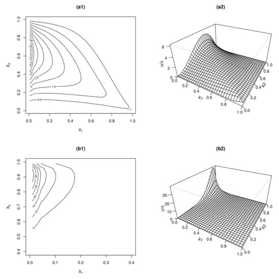
Figure 2. The contour plots and 3D perspectives of the bivariate NPIG distribution ${\mathrm{NPGA}}_2\left(\mathit{\varphi }\right)$ with different values of parameters: (a1,a2) $\mathit{\varphi }={(2,0.3,0.5)}^{\top }$; (b1,b2) $\mathit{\varphi }={(6,0.1,0.8)}^{\top }$.

3.2. ML Estimation of Parameters via the Gradient Descent Algorithm

Let ${\mathbf{x}}_1,\dots ,{\mathbf{x}}_n\stackrel{\mathrm{iid}}{\sim }{\mathrm{NPGA}}_2\left(\mathit{\varphi }\right)$ and $Y_{{\mathrm{obs}}_3}={\left\{{\mathit{x}}_i\right\}}_{i=1}^n$ denote the observed data, where ${\mathit{x}}_i={(x_{i1},x_{i2})}^{\top }$ is the realization of ${\mathbf{x}}_i={(X_{i1},X_{i2})}^{\top }$. The log-likelihood function of the parameter vector $\mathit{\varphi }$ is given by

$$\begin{array}{ccc}\hfill {\ell }_3\left(\mathit{\varphi }\right|Y_{{\mathrm{obs}}_3})& =& n\left[log\mathrm{\Gamma }\left(\frac{{\varphi }_0{\varphi }_1}{1-{\varphi }_1}+\frac{{\varphi }_0}{{\varphi }_2}\right)-log\mathrm{\Gamma }\left({\varphi }_0\right)-log\mathrm{\Gamma }\left(\frac{{\varphi }_0{\varphi }_1}{1-{\varphi }_1}\right)-log\mathrm{\Gamma }\left(\frac{{\varphi }_0}{{\varphi }_2}-{\varphi }_0\right)\right]\hfill \\ & & +\frac{{\varphi }_0{\varphi }_1}{1-{\varphi }_1}\sum _{i=1}^{n}log\frac{x_{i1}}{1-x_{i1}}+\left(\frac{{\varphi }_0}{{\varphi }_2}-{\varphi }_0\right)\sum _{i=1}^{n}log\frac{1-x_{i2}}{x_{i2}}\hfill \\ & & -\left(\frac{{\varphi }_0{\varphi }_1}{1-{\varphi }_1}+\frac{{\varphi }_0}{{\varphi }_2}\right)\sum _{i=1}^{n}log\left(1+\frac{x_{i1}}{1-x_{i1}}+\frac{1-x_{i2}}{x_{i2}}\right)+c_3,\hfill \end{array}$$

where $c_3$ is a constant free from the parameter vector $\mathit{\varphi }$. Then, we adopt the gradient descent algorithm directly to find the ML estimator $\widehat{\mathit{\varphi }}$ of $\mathit{\varphi }$ by setting

$$\nabla {\ell }_3\left(\mathit{\varphi }\right|Y_{{\mathrm{obs}}_3})\triangleq \frac{\partial {\ell }_3\left(\mathit{\varphi }\right|Y_{{\mathrm{obs}}_3})}{\partial \mathit{\varphi }}={\left(\frac{\partial {\ell }_3\left(\mathit{\varphi }\right|Y_{{\mathrm{obs}}_3})}{\partial {\varphi }_0},\frac{\partial {\ell }_3\left(\mathit{\varphi }\right|Y_{{\mathrm{obs}}_3})}{\partial {\varphi }_1},\frac{\partial {\ell }_3\left(\mathit{\varphi }\right|Y_{{\mathrm{obs}}_3})}{\partial {\varphi }_2}\right)}^{\top }.$$

Thus, the $(t+1)$-th estimation is given by

$${\mathit{\varphi }}^{(t+1)}={\mathit{\varphi }}^{\left(t\right)}+s_3^{\left(t\right)}\nabla {\ell }_3\left({\mathit{\varphi }}^{\left(t\right)}\right|Y_{{\mathrm{obs}}_3}),$$

(14)

where the step size at the t-th iteration is

$$s_3^{\left(t\right)}=\frac{|{[{\mathit{\varphi }}^{\left(t\right)}-{\mathit{\varphi }}^{(t-1)}]}^{\top }[\nabla {\ell }_3\left({\mathit{\varphi }}^{\left(t\right)}\right|Y_{{\mathrm{obs}}_3})-\nabla {\ell }_3\left({\mathit{\varphi }}^{(t-1)}\right|Y_{{\mathrm{obs}}_3})]|}{\parallel \nabla {\ell }_3\left({\mathit{\varphi }}^{\left(t\right)}\right|Y_{{\mathrm{obs}}_3})-\nabla {\ell }_3\left({\mathit{\varphi }}^{(t-1)}\right|Y_{{\mathrm{obs}}_3}){\parallel }^2}.$$

We also provide another method in Appendix B.2 with the N-EM algorithm applied, which results in the same iteration shown in (14).

3.3. Bivariate NPGA Mean Regression Model

The bivariate NPGA mean regression model is formulated in a similar way as

$$\left\{\begin{array}{c}{\mathbf{x}}_i={(X_{i1},X_{i2})}^{\top }\stackrel{\mathrm{ind}}{\sim }{\mathrm{NPGA}}_2({\varphi }_0,{\varphi }_{i1},{\varphi }_{i2}),i=1,\dots ,n,\hfill \\ {\displaystyle log\left({\displaystyle \frac{{\varphi }_{ij}}{1-{\varphi }_{ij}}}\right)={\mathit{v}}_i^{\top }{\mathit{\beta }}_j,\mathrm{or}{\varphi }_{ij}=\frac{exp\left({\mathit{v}}_i^{\top }{\mathit{\beta }}_j\right)}{1+exp\left({\mathit{v}}_i^{\top }{\mathit{\beta }}_j\right)},j=1,2,}\hfill \end{array}\right.$$

(15)

where ${\mathit{v}}_i={(1,v_{i1},\dots ,v_{iq})}^{\top }$ is the vector of covariates associated with the i-th subject, and ${\mathit{\beta }}_j={({\beta }_{0j},{\beta }_{1j},\dots ,{\beta }_{qj})}^{\top }$ is the $(q+1)$-vector of unknown regression coefficients. The gradient descent algorithm still works for finding the ML estimators of $\mathit{\phi }={({\varphi }_0,{\mathit{\beta }}_1^{\top },{\mathit{\beta }}_2^{\top })}^{\top }$ in the NPGA mean regression model, which is similar to that stated in Section 3.2.

4. Simulation Experiments

For all above bivariate NPIG- and NPGA-related models, although no explicit expressions for the ML estimators of parameters, the bootstrap method is an efficient tool to approximately calculate the standard errors and the confidence intervals (CIs) for them, while the details of the bootstrap procedure are omitted due to its routines. Based on it, we conduct several numerical experiments in the section to investigate the performances of the above-proposed estimation methods for the bivariate NPIG and NPGA distributions with their corresponding mean regression models. We use R software to design parallel computing on 64 CPUs of the windows system for the time-consuming simulations. The impacts of other computational aspects on the simulations are not considered.

4.1. Experiment for NPIG Models

Firstly, for the bivariate NPIG distribution, we choose the parameter configurations as follows: sample size is $n=30,50,100,300$; true values of $({\theta }_0,{\theta }_1,{\theta }_2)$ are set as $(1.2,0.3,0.8)$, $(0.5,0.5,0.6)$ and $(0.2,0.8,0.1)$, corresponding to a low, moderate and high correlations. In the regression model, the corresponding sample size is $n=50,200,350,500$; ${\theta }_0=0.6$, ${\mathit{\alpha }}_1={(1.2,0.8,-0.5,0.5)}^{\top }$, ${\mathit{\alpha }}_2={(1.5,-2,0.7,-0.5)}^{\top }$; the covariates are ${\mathit{w}}_i={(1,w_{i1},w_{i2},w_{i3})}^{\top }$, with $w_{i1}\stackrel{\mathrm{iid}}{\sim }\mathrm{Unif}(-1,1)$, $w_{i2}$ is randomly chosen from $\{0.2,0.4,0.6,0.8\}$ and $w_{i3}\stackrel{\mathrm{iid}}{\sim }\mathrm{Poisson}\left(3\right)$ for $i=1,\dots ,n$. For a given sample size n, experimental data ${\left\{{\mathit{x}}_i\right\}}_{i=1}^n$ are i.i.d. sampled from ${\mathrm{NPIG}}_2({\theta }_0,{\theta }_1,{\theta }_2)$ or each ${\mathit{x}}_i$ is generated from ${\mathrm{NPIG}}_2({\theta }_0,{\theta }_{i1},{\theta }_{i2})$ according to the regression model specified by (9), where SR (1) based on three IG variates can facilitate the sample generation. Parameters of interest are $({\theta }_0,{\theta }_1,{\theta }_2)$ and $({\theta }_0,{\mathit{\alpha }}_1,{\mathit{\alpha }}_2)$, respectively.

For each generated sample group, parameters are estimated by the proposed N-EM embedded with the gradient descent algorithm, and the whole process is repeated K times. The value of K is chosen as 1000 and 500 for the distribution and regression model, respectively. To better express the quantitative values on evaluating the estimation accuracy, we use a general symbol $\psi$ to denote each component of parameters to be estimated, and ${\psi }_0$ is its true value. The obtained ML estimate for $\psi$ in each loop is denoted by ${\widehat{\psi }}^{\left(k\right)}$, and the number of iterations is recorded as $t_k$ to the converged algorithm, where $k=1,\dots ,K$.

The averaged ML estimate (Ave-MLE), standard deviation (Std) and mean squared error (MSE) for the estimator $\widehat{\psi }$ and the averaged iterative number (it.no) are, respectively, computed as

$$\begin{array}{ccc}\hfill \mathrm{Ave-MLE}\left(\widehat{\psi }\right)& =& \frac{1}{K}\sum _{k=1}^K{\widehat{\psi }}^{\left(k\right)},\hfill \\ \hfill \mathrm{Std}\left(\widehat{\psi }\right)& =& \sqrt{\frac{1}{K-1}\sum _{k=1}^K{\left({\widehat{\psi }}^{\left(k\right)}-\frac{1}{K}\sum _{k=1}^K{\widehat{\psi }}^{\left(k\right)}\right)}^2},\hfill \\ \hfill \mathrm{MSE}\left(\widehat{\psi }\right)& =& {\left(\frac{1}{K}\sum _{k=1}^K{\widehat{\psi }}^{\left(k\right)}-{\psi }_0\right)}^2+\frac{1}{K-1}\sum _{k=1}^K{\left({\widehat{\psi }}^{\left(k\right)}-\frac{1}{K}\sum _{k=1}^K{\widehat{\psi }}^{\left(k\right)}\right)}^2,\hfill \\ \hfill \mathrm{it.no}& =& \frac{1}{K}\sum _{k=1}^K{t}_k.\hfill \end{array}$$

The simulated results for $({\theta }_0,{\theta }_1,{\theta }_2)$ of the bivariate NPIG distribution are summarized in Table 1. The simulated results for $({\theta }_0,{\mathit{\alpha }}_1,{\mathit{\alpha }}_2)$ of the bivariate NPIG regression model are listed in Table 2. From the results, it is easy to find that the estimates of the parameters are well provided and are much closer to their true values as the sample size increases; more specifically, the estimation stability and accuracy are both improved, as indicated by the decreasing values of Stds and MSEs. The population correlation coefficient and the averaged estimated value calculated with the ML estimates of parameters are also presented, which shows the relationship is completely depicted.

Table 1. ML estimate, Std and MSE for $({\theta }_0,{\theta }_1,{\theta }_2)$ in bivariate NPIG distribution.

(${\theta }_0,{\theta }_1,{\theta }_2)=(1.2,0.3,0.8),\rho =-0.2586$
Parameter	Ave-MLE	Std	MSE		Ave-MLE	Std	MSE
	$n=30$				$n=50$
${\theta }_0$	1.358641	0.442545	0.221013		1.316643	0.362304	0.144870
${\theta }_1$	0.298424	0.036809	0.001357		0.298486	0.028556	0.000818
${\theta }_2$	0.799534	0.031722	0.001007		0.801276	0.023760	0.000566
	it.no = 231, $\widehat{\rho }$ = −0.2569				it.no = 224, $\widehat{\rho }$ = −0.2564
	$n=100$				$n=300$
${\theta }_0$	1.243133	0.237282	0.058163		1.209933	0.121216	0.014792
${\theta }_1$	0.300323	0.020431	0.000418		0.300539	0.012035	0.000145
${\theta }_2$	0.799605	0.016497	0.000272		0.799794	0.009520	0.000091
	it.no = 213, $\widehat{\rho }$ = −0.2586				it.no = 197, $\widehat{\rho }$ = −0.2588
(${\theta }_0,{\theta }_1,{\theta }_2)=(0.5,0.5,0.6),\rho =-0.4390$
Parameter	Ave-MLE	Std	MSE		Ave-MLE	Std	MSE
	$n=30$				$n=50$
${\theta }_0$	0.566086	0.174171	0.034703		0.544802	0.128736	0.018580
${\theta }_1$	0.498231	0.048484	0.002354		0.499272	0.037687	0.001421
${\theta }_2$	0.601595	0.046221	0.002139		0.600750	0.035776	0.001280
	it.no = 172, $\widehat{\rho }$ = −0.4366				it.no = 167, $\widehat{\rho }$ = −0.4379
	$n=100$				$n=300$
${\theta }_0$	0.519031	0.085486	0.007670		0.504517	0.049257	0.002447
${\theta }_1$	0.500203	0.026148	0.000684		0.500225	0.015722	0.000247
${\theta }_2$	0.600492	0.025049	0.000628		0.599723	0.014972	0.000224
	it.no = 157, $\widehat{\rho }$ = −0.4386				it.no = 145, $\widehat{\rho }$ = −0.4391
(${\theta }_0,{\theta }_1,{\theta }_2)=(0.2,0.8,0.1),\rho =-0.7321$
Parameter	Ave-MLE	Std	MSE		Ave-MLE	Std	MSE
	$n=30$				$n=50$
${\theta }_0$	0.220128	0.055619	0.003499		0.211129	0.041009	0.001806
${\theta }_1$	0.800242	0.031396	0.000986		0.800302	0.022899	0.000524
${\theta }_2$	0.099971	0.018400	0.000339		0.099890	0.013603	0.000185
	it.no = 119, $\widehat{\rho }$ = −0.7350				it.no = 114, $\widehat{\rho }$ = −0.7338
	$n=100$				$n=300$
${\theta }_0$	0.205324	0.027086	0.000762		0.201148	0.015389	0.000238
${\theta }_1$	0.799645	0.016570	0.000275		0.800039	0.009393	0.000088
${\theta }_2$	0.100182	0.009942	0.000099		0.100087	0.005523	0.000031
	it.no = 107, $\widehat{\rho }$ = −0.7326				it.no = 97, $\widehat{\rho }$ = −0.7323

Table 2. ML estimate, Std and MSE for $({\theta }_0,{\mathit{\alpha }}_1,{\mathit{\alpha }}_2)$ in bivariate NPIG regression model.

${\theta }_0=0.6,{\mathit{\alpha }}_1={(1.2,0.8,-0.5,0.5)}^{\top },{\mathit{\alpha }}_2={(1.5,-2,0.7,-0.5)}^{\top }$
Parameter	Ave-MLE	Std	MSE		Ave-MLE	Std	MSE
	$n=50$				$n=200$
${\theta }_0$	0.616064	0.098125	0.009887		0.594675	0.054724	0.003023
${\alpha }_{01}$	1.197065	0.182278	0.033234		1.202689	0.051280	0.002637
${\alpha }_{11}$	0.791274	0.159555	0.025534		0.797376	0.050753	0.002583
${\alpha }_{21}$	−0.503090	0.172935	0.029916		−0.501269	0.052572	0.002765
${\alpha }_{31}$	0.496402	0.052044	0.002721		0.495028	0.022855	0.000547
${\alpha }_{02}$	1.493490	0.172693	0.029865		1.493448	0.059934	0.003635
${\alpha }_{12}$	−1.994148	0.159105	0.025349		−1.994163	0.055346	0.003097
${\alpha }_{22}$	0.693314	0.189516	0.035961		0.695733	0.044827	0.002028
${\alpha }_{32}$	−0.497199	0.051602	0.002671		−0.496026	0.023453	0.000566
	it.no = 141				it.no = 68
	$n=350$				$n=500$
${\theta }_0$	0.594409	0.040014	0.001632		0.592610	0.034314	0.001232
${\alpha }_{01}$	1.199199	0.032275	0.001042		1.200771	0.021140	0.000447
${\alpha }_{11}$	0.795187	0.036466	0.001353		0.798587	0.025180	0.000636
${\alpha }_{21}$	−0.500220	0.028680	0.000823		−0.500038	0.021437	0.000460
${\alpha }_{31}$	0.499380	0.019778	0.000392		0.496742	0.018138	0.000340
${\alpha }_{02}$	1.494840	0.035134	0.001261		1.495448	0.025697	0.000681
${\alpha }_{12}$	−1.997357	0.033092	0.001102		−1.997702	0.025642	0.000663
${\alpha }_{22}$	0.698411	0.028526	0.000816		0.697747	0.020047	0.000407
${\alpha }_{32}$	−0.498473	0.019025	0.000364		−0.497432	0.015664	0.000252
	it.no = 55				it.no = 49

4.2. Experiments for NPGA Models

For the bivariate NPGA distribution, the parameter settings are similar with those for the NPIG models. The choice of sample size n is the same. True values of $({\varphi }_0,{\varphi }_1,{\varphi }_2)$ are chosen as $(2,0.9,0.2)$ and $(5,0.4,0.6)$ for the NPGA distribution. In the NPGA regression model, ${\varphi }_0=1.2$, ${\mathit{\beta }}_1={(-0.9,1.4,-0.5)}^{\top }$, ${\mathit{\beta }}_2={(0.5,-0.2,-0.8)}^{\top }$; the covariates are ${\mathit{v}}_i={(1,v_{i1},v_{i2})}^{\top }$, with $v_{i1}\stackrel{\mathrm{iid}}{\sim }\mathrm{Unif}(0,1)$, and $v_{i2}$ is randomly sampled from $\{-0.5,-0.2,0.3,0.6\}$ for $i=1,\dots ,n$. Data ${\left\{{\mathit{x}}_i\right\}}_{i=1}^n$ are generated from ${\mathrm{NPGA}}_2({\varphi }_0,{\varphi }_1,{\varphi }_2)$ or ${\mathrm{NPGA}}_2({\varphi }_0,{\varphi }_{i1},{\varphi }_{i2})$ according to the model specified by (15). To assess the estimation performances on parameters of interest $({\varphi }_0,{\varphi }_1,{\varphi }_2)$ and $({\varphi }_0,{\mathit{\beta }}_1,{\mathit{\beta }}_2)$, we still adopt the measurements introduced in Section 4.1 for comparisons.

Table 3 and Table 4 summarize the results of simulation studies for the bivariate NPGA distribution and the corresponding mean regression model. The averaged ML estimates are provided, as well as the Stds and MSEs of the estimators. It is also observed that the estimation performance is satisfactory. The values of iterative numbers indicate that the computational efficiency and convergence rate are good. All averaged estimated values of the correlation calculated with the ML estimates of parameters are close to the population correlation coefficients.

Table 3. ML estimate, Std and MSE for $({\varphi }_0,{\varphi }_1,{\varphi }_2)$ in bivariate NPGA distribution.

$({\varphi }_0,{\varphi }_1,{\varphi }_2)=(2,0.9,0.2),\rho =-0.8083$
Parameter	Ave-MLE	Std	MSE		Ave-MLE	Std	MSE
	$n=30$				$n=50$
${\varphi }_0$	1.997760	0.026205	0.000692		1.998313	0.023109	0.000537
${\varphi }_1$	0.898923	0.010484	0.000111		0.899695	0.008393	0.000071
${\varphi }_2$	0.202299	0.019508	0.000386		0.200620	0.015605	0.000244
	it.no = 27, $\widehat{\rho }$ = −0.8064				it.no = 27, $\widehat{\rho }$ = −0.8078
	$n=100$				$n=300$
${\varphi }_0$	1.999660	0.024147	0.000583		1.998969	0.020451	0.000419
${\varphi }_1$	0.900010	0.005360	0.000029		0.899674	0.003072	0.000010
${\varphi }_2$	0.201871	0.010523	0.000114		0.201171	0.006473	0.000043
	it.no = 26, $\widehat{\rho }$ = −0.8072				it.no = 27, $\widehat{\rho }$ = −0.8074
$({\varphi }_0,{\varphi }_1,{\varphi }_2)=(5,0.4,0.6),\rho =-0.4057$
Parameter	Ave-MLE	Std	MSE		Ave-MLE	Std	MSE
	$n=30$				$n=50$
${\varphi }_0$	5.001001	0.036186	0.001310		4.998937	0.032888	0.001083
${\varphi }_1$	0.402014	0.026780	0.000721		0.402845	0.020853	0.000443
${\varphi }_2$	0.598549	0.026008	0.000679		0.598827	0.020339	0.000415
	it.no = 21, $\widehat{\rho }$ = −0.4069				it.no = 21, $\widehat{\rho }$ = −0.4074
	$n=100$				$n=300$
${\varphi }_0$	4.996352	0.042099	0.001786		5.001158	0.038537	0.001486
${\varphi }_1$	0.400435	0.015158	0.000230		0.399487	0.008230	0.000068
${\varphi }_2$	0.599306	0.015034	0.000227		0.600232	0.007946	0.000063
	it.no = 21, $\widehat{\rho }$ = −0.4061				it.no = 16, $\widehat{\rho }$ = −0.4053

Table 4. ML estimate, Std and MSE for $({\varphi }_0,{\mathit{\beta }}_1,{\mathit{\beta }}_2)$ in bivariate NPGA regression model.

${\varphi }_0=1.2,{\mathit{\beta }}_1={(-0.9,1.4,-0.5)}^{\top },{\mathit{\beta }}_2={(0.5,-0.2,-0.8)}^{\top }$
Parameter	Ave-MLE	Std	MSE		Ave-MLE	Std	MSE
	$n=50$				$n=200$
${\varphi }_0$	1.273002	0.200704	0.045612		1.227011	0.092474	0.009281
${\beta }_{01}$	−0.863261	0.274594	0.076752		−0.860950	0.137262	0.020366
${\beta }_{11}$	1.374930	0.482249	0.233192		1.341559	0.226420	0.054681
${\beta }_{21}$	−0.489769	0.324336	0.105299		−0.481630	0.147419	0.022070
${\beta }_{02}$	0.437918	0.290704	0.088363		0.4730029	0.140378	0.020435
${\beta }_{12}$	−0.146745	0.492742	0.245631		−0.177881	0.230247	0.053503
${\beta }_{22}$	−0.784241	0.340255	0.116021		−0.773613	0.157350	0.025455
	it.no = 51				it.no = 44
	$n=350$				$n=500$
${\varphi }_0$	1.218954	0.072089	0.005556		1.210845	0.028854	0.000950
${\beta }_{01}$	−0.867234	0.106863	0.012493		−0.867112	0.042890	0.002921
${\beta }_{11}$	1.362347	0.170824	0.030598		1.353711	0.068964	0.006899
${\beta }_{21}$	−0.486299	0.120704	0.014757		−0.486765	0.048496	0.002527
${\beta }_{02}$	0.467544	0.101781	0.011413		0.476607	0.042584	0.002361
${\beta }_{12}$	−0.168965	0.166065	0.028541		−0.174730	0.069102	0.005414
${\beta }_{22}$	−0.772744	0.117103	0.014456		−0.777010	0.049669	0.002996
	it.no = 42				it.no = 36

4.3. Numerical Study on Means, Variances, Covariances and Correlations

In this subsection, we provide some numerical studies on the means, variances, covariances and correlations. For the bivariate NPIG distribution, we choose the values of mean parameters as $({\theta }_1,{\theta }_2)=(0.5,0.6),(0.3,0.8),(0.8,0.1)$, combined with the value of ${\theta }_0$ being $0.2,0.4,0.6,0.8,1,3,5,10,15$ and 20, respectively. The expectations, variances for two components, the covariances, and the correlation coefficients between them are presented in Table 5. For the bivariate NPGA distribution, we choose the values of the mean parameters as $({\varphi }_1,{\varphi }_2)=(0.9,0.2),(0.4,0.7),(0.2,0.2)$, combined with the value of ${\varphi }_0$ being the same as that of ${\theta }_0$. The corresponding properties are summarized in Table 6. Note that the expectation for each component is just ${\theta }_i$ or ${\varphi }_i$ for $i=1,2$ in the two distributions. “Mean1” indicates the expectation for the first component, and “Mean2” indicates the expectation for the second component. Variances and covariances are computed based on the derived formulae in the Section 2.1 and Section 3.1, respectively, and “Var1” indicates the variance for the first component, “Var2” indicates the variance for the second component and “Cov” indicates the covariance between the two components. The correlation coefficient indicated by “Coef” is calculated according to its definition.

Table 5. Means, variances, covariances and correlations for the bivariate NPIG distribution.

${\mathit{\theta }}_0$	Mean1	Mean2	Var1	Var2	Cov	Coef
0.2	0.5	0.6	0.095957	0.095424	−0.041228	−0.430854
0.4	0.5	0.6	0.080300	0.081386	−0.035332	−0.437049
0.6	0.5	0.6	0.069668	0.071562	−0.031100	−0.440454
0.8	0.5	0.6	0.061796	0.064130	−0.027863	−0.442600
1	0.5	0.6	0.055664	0.058245	−0.025285	−0.444056
3	0.5	0.6	0.028704	0.031267	−0.013426	−0.448160
5	0.5	0.6	0.019542	0.021624	−0.009222	−0.448594
10	0.5	0.6	0.010927	0.012291	−0.005197	−0.448441
15	0.5	0.6	0.007596	0.008602	−0.003623	−0.448208
20	0.5	0.6	0.005823	0.006620	−0.002782	−0.448038
0.2	0.3	0.8	0.085745	0.066704	−0.019270	−0.254800
0.4	0.3	0.8	0.074236	0.058458	−0.016938	−0.257123
0.6	0.3	0.8	0.065981	0.052423	−0.015181	−0.258120
0.8	0.3	0.8	0.059627	0.047708	−0.013789	−0.258536
1	0.3	0.8	0.054527	0.043879	−0.012652	−0.258650
3	0.3	0.8	0.030294	0.025118	−0.007072	−0.256390
5	0.3	0.8	0.021249	0.017844	−0.004950	−0.254195
10	0.3	0.8	0.012261	0.010441	−0.002841	−0.251100
15	0.3	0.8	0.008637	0.007400	−0.001995	−0.249545
20	0.3	0.8	0.006671	0.005735	−0.001538	−0.248617
0.2	0.8	0.1	0.047708	0.020039	−0.022637	−0.732127
0.4	0.8	0.1	0.035625	0.013569	−0.016702	−0.759669
0.6	0.8	0.1	0.028700	0.010334	−0.013357	−0.775590
0.8	0.8	0.1	0.024122	0.008365	−0.011170	−0.786306
1	0.8	0.1	0.020844	0.007035	−0.009616	−0.794114
3	0.8	0.1	0.008965	0.002734	−0.004079	−0.823825
5	0.8	0.1	0.005735	0.001700	−0.002599	−0.832436
10	0.8	0.1	0.003022	0.000874	−0.001365	−0.839907
15	0.8	0.1	0.002052	0.000588	−0.000926	−0.842639
20	0.8	0.1	0.001554	0.000443	−0.000701	−0.844056

Table 6. Means, variances, covariances and correlations for the bivariate NPGA distribution.

${\mathit{\varphi }}_0$	Mean1	Mean2	Var1	Var2	Cov	Coef
0.2	0.9	0.2	0.030000	0.080000	−0.031973	−0.652641
0.4	0.9	0.2	0.018000	0.053333	−0.022113	−0.713705
0.6	0.9	0.2	0.012857	0.040000	−0.016892	−0.744877
0.8	0.9	0.2	0.010000	0.032000	−0.013669	−0.764106
1	0.9	0.2	0.008182	0.026667	−0.011480	−0.777230
3	0.9	0.2	0.002903	0.010000	−0.004421	−0.820416
5	0.9	0.2	0.001765	0.006154	−0.002738	−0.830996
10	0.9	0.2	0.000891	0.003137	−0.001404	−0.839489
15	0.9	0.2	0.000596	0.002105	−0.000944	−0.842438
20	0.9	0.2	0.000448	0.001584	−0.000711	−0.843936
0.2	0.4	0.7	0.180000	0.163333	−0.052559	−0.306532
0.4	0.4	0.7	0.144000	0.133636	−0.045743	−0.329747
0.6	0.4	0.7	0.120000	0.113077	−0.039804	−0.341705
0.8	0.4	0.7	0.102857	0.098000	−0.034977	−0.348383
1	0.4	0.7	0.090000	0.086471	−0.031078	−0.352290
3	0.4	0.7	0.040000	0.039730	−0.014237	−0.357122
5	0.4	0.7	0.025714	0.025789	−0.009141	−0.354974
10	0.4	0.7	0.013585	0.013738	−0.004805	−0.351719
15	0.4	0.7	0.009231	0.009363	−0.003256	−0.350212
20	0.4	0.7	0.006990	0.007101	−0.002462	−0.349366
0.2	0.2	0.2	0.128000	0.080000	−0.026476	−0.261637
0.4	0.2	0.2	0.106667	0.053333	−0.022288	−0.295506
0.6	0.2	0.2	0.091429	0.040000	−0.019121	−0.316183
0.8	0.2	0.2	0.080000	0.032000	−0.016708	−0.330219
1	0.2	0.2	0.071111	0.026667	−0.014822	−0.340368
3	0.2	0.2	0.033684	0.010000	−0.006910	−0.376481
5	0.2	0.2	0.022069	0.006154	−0.004494	−0.385587
10	0.2	0.2	0.011852	0.003137	−0.002395	−0.392746
15	0.2	0.2	0.008101	0.002105	−0.001632	−0.395167
20	0.2	0.2	0.006154	0.001584	−0.001238	−0.396378

5. Applications

We obtain the cortical thickness of 41 patients with schizophrenia and 40 healthy controls from [18]. Structural magnetic resonance imaging scans obtained from the participants were processed using Freesurfer. Cortical thickness was parcellated by the Destrieux atlas [19] to provide 148 brain regions and estimated by the standard procedures described in [20]. Regional Ethics Committees (Nottinghamshire & Derbyshire) approved the study and all participants provided written informed consent. We aim to analyze the negative co-varying pairs of regions for investigating the influence of schizophrenia on the cortical thickness between controls and patients. The negative correlation pairs among 148 dimensions of data based on Pearson correlation coefficients are shown in Figure 3. The locations of squares marked with red circles are our following examples in subsections. The descriptions of used data are given in the Supplementary Material.

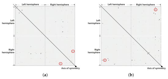
Figure 3. Negative correlations between the thickness of 74 different sulco-gyral cortical units in each hemisphere of (a) patients; (b) controls. (Each square represent a negative correlation of corresponding units under the Spearman significance test, where the p-values of black ones are $p<0.01$ and gray ones are $0.01⩽p<0.05$).

5.1. Lateral and Suborbital Sulcus

We take the thickness difference of the horizontal ramus of the anterior segment of the lateral sulcus ($X_1$) and suborbital sulcus ($X_2$) in the right hemisphere as $\mathbf{x}={(X_1,X_2)}^{\top }$. Based on the significant, negative correlation between $X_1$ and $X_2$ in patients and a positive correlation in controls, we fit the patient and control groups data into the four different distributions, where bivariate PIG and PGA models are derived from [16]. The $95\%$ CIs and Stds of parameters (Par.) are calculated by bootstrap re-samplings.

The results are shown in Table 7. We note that the bivariate PGA and NPGA distributions perform better under the model selection criterion. The ML estimates of the mean parameters in two distributions between the patient and control groups fall on the boundary of the corresponding parameters’ confidence intervals of the other group, respectively. This implies the different cortical thinness between the two groups. Although the two regions inhibited each other, their thicknesses in the patients were significantly reduced compared with the control group. With the weakening of the compensatory behaviors of the patients’ cortical thickness in these areas, the negatively correlated pair different from the control group was produced, which is consistent with the clinical manifestations of changes in the cerebral cortex of schizophrenia.

Table 7. ML estimates (MLEs), stds and CIs for the thickness of $X_1$ and $X_2$ (Section 5.1) between controls and patients in two distributions with model selection criterion AIC and BIC.

Par.	Controls			Patients
	MLE	CI	Std	MLE	CI	Std
	Bivariate PIG distribution			Bivariate NPIG distribution
${\theta }_0$	0.4296	[0.2744, 0.7503]	0.1242	0.4837	[0.3158, 0.8444]	0.1370
${\theta }_1$	0.4664	[0.3821, 0.5473]	0.0416	0.4249	[0.3504, 0.5042]	0.0399
${\theta }_2$	0.5029	[0.4213, 0.5877]	0.0427	0.4209	[0.3438, 0.4923]	0.0378
	AIC = 18.0480; BIC = 23.1147			AIC = 1.4008; BIC = 6.5415
	Bivariate PGA distribution			Bivariate NPGA distribution
${\varphi }_0$	1.4540	[1.0527, 2.0820]	0.2606	1.5477	[1.2360, 1.8403]	0.1418
${\varphi }_1$	0.5071	[0.4317, 0.5812]	0.0373	0.4294	[0.3659, 0.5023]	0.0359
${\varphi }_2$	0.5161	[0.4454, 0.5881]	0.0383	0.4059	[0.3394, 0.4676]	0.0319
	AIC = 2.0847; BIC = 7.1514			AIC = −9.9734; BIC = −4.8327

To further study the thickness changes in patients, we introduce two common covariates for the two groups: $w_{i1}$, $v_{i1}$ are the logarithm transformation of the age in years, and $w_{i2}$, $v_{i2}$ are gender (male=0, female=1). Based on (9) and (15), we have the following regression models:

$$log\left({\displaystyle \frac{{\mu }_{ij}}{1-{\mu }_{ij}}}\right)={\alpha }_{j0}+{\alpha }_{j1}{w}_{i1}+{\alpha }_{j2}{w}_{i2}\mathrm{and}log\left({\displaystyle \frac{{\varphi }_{ij}}{1-{\varphi }_{ij}}}\right)={\beta }_{j0}+{\beta }_{j1}{v}_{i1}+{\beta }_{j2}{v}_{i2},$$

where $i=1,\dots ,n$, and $j=1,2$. Table 8 listed the results by fitting the data of patients and controls with the four corresponding regression models. From the $95\%$ bootstrap CIs, we know that there are significantly negative relationships between $\mathbf{x}$ and log(age) only in controls. The other difference is focused on the influence of gender to $X_2$, which is significantly positive to $X_2$ in controls and indicates irrelevant to $X_2$ in patients. Based on the results, we see that the mutual inhibition between $X_1$ and $X_2$ is mainly due to the opposite compensation of $X_1$ with gender and $X_2$ with age in patients.

Table 8. ML estimates (MLEs), stds and CIs for the thickness of $X_1$ and $X_2$ (Section 5.1) between controls and patients in two regression models with selection criterion AIC and BIC.

Par.	Controls			Patients
	MLE	CI	Std	MLE	CI	Std
	Bivariate PIG mean regression			Bivariate NPIG mean regression
${\theta }_0$	0.5588	[0.3899, 1.0599]	0.1789	0.5355	[0.4019, 1.0499]	0.1579
${\alpha }_{10}$	4.9412	[1.7141, 8.1186]	1.6109	2.6217	[−1.0682, 6.7279]	1.8809
${\alpha }_{11}$	−1.5045	[−2.4762, −0.6009]	0.4686	−0.8339	[−2.0480, 0.2186]	0.5428
${\alpha }_{12}$	0.6536	[0.0220, 1.4045]	0.3506	−0.0466	[−0.7188, 0.7475]	0.3654
${\alpha }_{20}$	4.0251	[0.7731, 7.6577]	1.6832	0.4262	[−3.5984, 4.4486]	1.8909
${\alpha }_{21}$	−1.1637	[−2.2148, −0.2369]	0.4891	−0.2414	[−1.3743, 0.8807]	0.5476
${\alpha }_{22}$	0.1555	[−0.4933, 0.8664]	0.3469	0.3114	[−0.5136, 0.9808]	0.3816
	AIC = 15.0705; BIC = 26.8926			AIC = 4.6480; BIC = 16.6430
	Bivariate PGA mean regression			Bivariate NPGA mean regression
${\varphi }_0$	1.5535	[1.1976, 2.2985]	0.2744	1.6295	[1.2301, 2.5405]	0.3288
${\beta }_{10}$	6.1568	[4.3330, 7.6466]	0.7389	1.4482	[−1.7922, 5.0879]	1.7278
${\beta }_{11}$	−1.7962	[−2.2712, −1.2685]	0.2251	−0.4871	[−1.5415, 0.4178]	0.4990
${\beta }_{12}$	0.4822	[0.0032, 1.0710]	0.2857	−0.1693	[−0.7979, 0.4999]	0.3374
${\beta }_{20}$	4.8569	[3.3534, 6.5856]	0.7110	1.8815	[−1.3326, 4.7364]	1.5787
${\beta }_{21}$	−1.3976	[−1.9201, −0.9069]	0.2127	−0.6746	[−1.5283, 0.2427]	0.4539
${\beta }_{22}$	0.2720	[−0.2365, 0.9072]	0.2990	0.3070	[−0.2977, 0.8459]	0.3052
	AIC = 4.2536; BIC = 16.0757			AIC = −6.7527; BIC = 5.2424

Summarizing the results in Table 7 and Table 8, we think the causes of these features, such as the effect of drug dose on different genders or the variable changes of brain regions with the durations, still need to be further explored.

5.2. Cingulate Gyrus and Lateral Occipito-Temporal Sulcus

In this subsection, we analyze regions in different hemispheres. The left posterior-dorsal part of the cingulate gyrus ($X_1$) and right lateral occipito-temporal sulcus ($X_2$) are taken as $\mathit{x}={(X_1,X_2)}^{\top }$. Based on the significant negative correlation between $X_1$ and $X_2$ in controls and a positive correlation in patients, we fit the data of patients and controls into the four distributions, respectively. Similar to Section 5.1, we also consider covariates in four corresponding mean regression models. The correlation information from the samples implies that the data are not related to gender, so we only consider one covariate log(age). The results are summarized in Table 9 and Table 10.

Table 9. ML estimates (MLEs), stds and CIs for the thickness of $X_1$ and $X_2$ (Section 5.2) between controls and patients in two distributions with model selection criterion AIC and BIC.

Par.	Patients			Controls
	MLE	CI	Std	MLE	CI	Std
	Bivariate PIG distribution			Bivariate NPIG distribution
${\theta }_0$	0.6307	[0.4001, 1.1844]	0.1903	1.6761	[1.1946, 2.6281]	0.3711
${\theta }_1$	0.4010	[0.3243, 0.4790]	0.0396	0.5031	[0.4390, 0.5676]	0.0325
${\theta }_2$	0.4552	[0.3859, 0.5331]	0.0386	0.5215	[0.4614, 0.5843]	0.0320
	AIC = 4.1243; BIC = 9.2650			AIC = −29.0117; BIC = −23.9451
	Bivariate PGA distribution			Bivariate NPGA distribution
${\varphi }_0$	1.9787	[1.5283, 2.8760]	0.3586	3.0165	[2.8431, 3.1387]	0.0711
${\varphi }_1$	0.3967	[0.3249, 0.4524]	0.0334	0.5000	[0.4531, 0.5639]	0.0267
${\varphi }_2$	0.4650	[0.4009, 0.5221]	0.0334	0.5374	[0.4771, 0.5886]	0.0273
	AIC = −12.8517; BIC = −7.7109			AIC = −43.0450; BIC = −37.9783

Table 10. ML estimates (MLEs), stds and CIs for the thickness of $X_1$ and $X_2$ (Section 5.2) between controls and patients in two regression models with selection criterion AIC and BIC.

Par.	Patients			Controls
	MLE	CI	Std	MLE	CI	Std
	Bivariate PIG mean regression			Bivariate NPIG mean regression
${\theta }_0$	0.7825	[0.5220, 1.3723]	0.2194	1.8085	[1.3285, 2.8110]	0.3876
${\alpha }_{10}$	3.4074	[0.3196, 6.1716]	1.5023	3.2295	[0.3851, 6.4295]	1.5459
${\alpha }_{11}$	−1.0921	[−1.9158, −0.2041]	0.4349	−0.9194	[−1.8404, −0.0923]	0.4459
${\alpha }_{20}$	3.6225	[0.4132, 6.5227]	1.5104	−0.1836	[−2.8446, 2.9085]	1.4255
${\alpha }_{21}$	−1.0925	[−1.9570, −0.1878]	0.4373	0.0806	[−0.8328, 0.8209]	0.4091
	AIC = 0.0722; BIC = 8.6400			AIC = −31.1357; BIC = −22.6913
	Bivariate PGA mean regression			Bivariate NPGA mean regression
${\varphi }_0$	2.1331	[1.6301, 3.0572]	0.3632	3.2817	[2.5071, 4.8420]	0.6160
${\beta }_{10}$	3.0007	[1.0820, 4.6351]	0.7655	3.2619	[0.4007, 6.0649]	1.4288
${\beta }_{11}$	−0.9823	[−1.4382, −0.4542]	0.2243	−0.9366	[−1.7524, −0.1013]	0.4134
${\beta }_{20}$	2.6646	[0.8734, 4.2967]	0.8151	−0.0168	[−2.9359, 2.9117]	1.5148
${\beta }_{21}$	−0.8051	[−1.3183, −0.3098]	0.2397	0.0486	[−0.8062, 0.8667]	0.4337
	AIC = −16.1259; BIC = −7.5581			AIC = −46.5825; BIC = −38.1381

Based on the selection criterion, bivariate PGA and NPGA distributions and models show better performance. The mean cortical thickness differences between the two groups are significant. Similar to the results of medical research, the thicknesses in patients were consistently smaller than those of the controls. In the mean regression models, the influences of log(age) to $\mathbf{x}$ are quite similar in the two groups, which is obviously different from the results shown in the previous subsection. The slight difference between the two groups is the influence of log(age) to $X_2$, which is not significant in controls.

Combining the results in the two tables, we find the thickness difference between the two groups due to the loss of compensatory behaviors in the patients and raise a reasonable doubt that the duration of patients may cause the loss.

6. Conclusions, Limitations, and Future Research

In this paper, we proposed models that fit bivariate negatively correlated continuous proportional data for the first time. Based on the equal-dispersed IG distribution and the gamma distribution with a single parameter, we developed the bivariate NPIG and NPGA distributions. Models with covariates are also considered by formulating the mean regression models based on the two new distributions. Moreover, we provide efficient methods for parameter estimations of the four different models, respectively. The N-EM algorithm aided by the gradient descent algorithms based on Jensen’s inequality is used to overcome the difficulties in calculating ML estimates of parameters. For readers interested in algorithms, we recommend reading [21,22]. In Section 5, we used two different criteria to evaluate the models. We study the negative correlation pairs that increase with the decrease in compensation behaviors, and the information obtained from the main research is consistent with our previous findings with the same dataset [23]. Moreover, we propose the hypotheses of the causes of them based on the results, which needs further medical exploration. According to our analysis of the cortical thickness of schizophrenic patients and the control group, we verified the compensatory nature of cortical thickness in schizophrenic patients and found that it was negatively correlated with age. If you want to use the original data and R code of this article for your research, please contact the corresponding author by email. In addition, the use of original data should be agreed with the data collection team.

There are other topics worthy of further research beyond this paper. We only considered the mean regression models for the proposed distributions and did not consider the mode regressions as there are no closed forms for their modes. Similarly, there are quantile regressions. To better interpret the data, we hope to explore the mode regression models and have already constructed a new model with an explicit expression of the mode. The construction structure is $1/(1+Y)$ similar to (1). Moreover, linear constructions, such as SR (1), to set models with arbitrary positive or negative correlations are difficult to achieve. We consider changing independent ${\left\{Y_j\right\}}_{j=1}^2$ to a bivariate correlated vector $\mathbf{y}={(Y_1,Y_2)}^{\top }$ and then the correlation structure between components based on the construction (1) more flexible. Moreover, the Copula method may be one feasible way, or mixture models could be considered by combining PIG with NPIG and PGA with NPGA. Finally, the exact tests in the bivariate NPIG and NPGA models for one sample and multiple samples are also our interests. They can help us research the significance of differences.

References

- Ferrari, S.; Cribari-Neto, F. Beta regression for modelling rates and proportions. J. Appl. Stat. 2004, 31, 799–815. [Google Scholar] [CrossRef]
- Simas, A.B.; Barreto-Souza, W.; Rocha, A.V. Improved estimators for a general class of beta regression models. Comput. Stat. Data Anal. 2010, 54, 348–366. [Google Scholar] [CrossRef] [Green Version]
- Ferrari, S.L.P.; Pinheiro, E.C. Improved likelihood inference in beta regression. J. Stat. Comput. Simul. 2011, 81, 431–443. [Google Scholar] [CrossRef]
- Kieschnick, R.; McCullough, B.D. Regression analysis of variates observed on (0, 1): Percentages, proportions and fractions. Stat. Model. 2003, 3, 193–213. [Google Scholar] [CrossRef] [Green Version]
- Zhang, P.; Qiu, Z.G. Regression analysis of proportional data using simplex distribution. Sci. Sin. Math. 2014, 44, 89–104. (In Chinese) [Google Scholar] [CrossRef] [Green Version]
- Lijoi, A.; Mena, R.H.; Prünster, I. Hierarchical mixture modeling with normalized inverse–Gaussian priors. J. Am. Stat. Assoc. 2005, 100, 1278–1291. [Google Scholar] [CrossRef]
- Liu, P.Y.; Tian, G.L.; Yuen, K.C.; Zhang, C.; Tang, M.L. Proportional inverse Gaussian distribution: A new tool for analyzing continuous proportional data. Aust. N. Z. J. Stat. 2021, (in press). [Google Scholar] [CrossRef]
- Wang, C.; Tu, D. A bootstrap semiparametric homogeneity test for the distributions of multigroup proportional data, with applications to analysis of quality of life outcomes in clinical trials. Stat. Med. 2020, 39, 1715–1731. [Google Scholar] [CrossRef]
- Connor, R.J.; Mosimann, J.E. Concepts of independence for proportions with a generalization of the Dirichlet distribution. J. Am. Stat. Assoc. 1969, 64, 194–206. [Google Scholar] [CrossRef]
- Campbell, G.; Mosimann, J.E. Multivariate methods for proportional shape. ASA Proc. Sect. Stat. Graph. 1987, 1, 10–17. [Google Scholar]
- Gueorguieva, R.; Rosenheck, R.; Zelterman, D. Dirichlet component regression and its applications to psychiatric data. Comput. Stat. Data Anal. 2008, 52, 5344–5355. [Google Scholar] [CrossRef] [PubMed] [Green Version]
- Zhang, B. On Compositional Data Modeling and Its Biomedical Applications. Ph.D. Dissertation, Columbia University, New York, NY, USA, 2013. [Google Scholar]
- Morais, J.; Thomas-Agnan, C.; Simioni, M. Using compositional and Dirichlet models for market share regression. J. Appl. Stat. 2018, 45, 1670–1689. [Google Scholar] [CrossRef] [Green Version]
- Cepeda-Cuervo, E.; Achcar, J.A.; Lopera, L.G. Bivariate beta regression models: Joint modeling of the mean, dispersion and association parameters. J. Appl. Stat. 2014, 41, 677–687. [Google Scholar] [CrossRef]
- Petterle, R.R.; Laureano, H.A.; da Silva, G.P.; Bonat, W.H. Multivariate generalized linear mixed models for continuous bounded outcomes: Analyzing the body fat percentage data. Stat. Methods Med. Res. 2021, 30, 2619–2633. [Google Scholar] [CrossRef] [PubMed]
- Sun, Y.; Tian, G.L.; Guo, S.X.; Liu, P.Y. New models for analyzing positively correlated continuous proportional data: A cortical thickness study for schizophrenia. Biometrics 2021. (submitted). [Google Scholar]
- Tweedie, M.C.K. Statistical properties of inverse Gaussian distributions. I. Ann. Math. Stat. 2018, 28, 362–377. [Google Scholar] [CrossRef]
- Palaniyappan, L.; Liddle, P.F. Diagnostic discontinuity in psychosis: A combined study of cortical gyrification and functional connectivity. Schizophr. Bull. 2014, 40, 675–684. [Google Scholar] [CrossRef]
- Destrieux, C.; Fischl, B.; Dale, A.; Halgren, E. Automatic parcellation of human cortical gyri and sulci using standard anatomical nomenclature. NeuroImage 2010, 53, 1–15. [Google Scholar] [CrossRef] [Green Version]
- Fischl, B.; Dale, A.M. Measuring the thickness of the human cerebral cortex from magnetic resonance images. Proc. Natl. Acad. Sci. USA 2000, 97, 11050–11055. [Google Scholar] [CrossRef] [Green Version]
- McLachlan, G.J.; Krishnan, T. The EM Algorithm and Extensions, 2nd ed.; John Wiley & Sons: New York, NY, USA, 2007. [Google Scholar]
- Lange, K. MM Optimization Algorithms; Society for Industrial and Applied Mathematics: Philadelphia, PA, USA, 2016. [Google Scholar]
- Guo, S.X.; Palaniyappan, L.; Liddle, F.P.; Feng, J.F. Dynamic cerebral reorganization in the pathophysiology of schizophrenia: A MRI-derived cortical thickness study. Psychol. Med. 2016, 46, 2201–2214. [Google Scholar]
- Lange, K.; Hunter, D.R.; Yang, I. Optimization transfer using surrogate objective functions (with discussions). J. Comput. Graph. Stat. 2000, 9, 1–20. [Google Scholar]
- Hunter, D.R.; Lange, K. A tutorial on MM algorithms. Am. Stat. 2004, 58, 30–37. [Google Scholar] [CrossRef]
- Tian, G.L.; Huang, X.F.; Xu, J.F. An assembly and decomposition approach for constructing separable minorizing functions in a class of MM algorithms. Stat. Sin. 2004, 29, 961–982. [Google Scholar] [CrossRef] [Green Version]
Publisher’s Note: MDPI stays neutral with regard to jurisdictional claims in published maps and institutional affiliations. |
© 2022 by the authors. Licensee MDPI, Basel, Switzerland. This article is an open access article distributed under the terms and conditions of the Creative Commons Attribution (CC BY) license (https://creativecommons.org/licenses/by/4.0/).