Towards Distributed Lexicographically Fair Resource Allocation with an Indivisible Constraint

Abstract

In the cloud computing and big data era, data analysis jobs are usually executed over geo-distributed data centers to make use of data locality. When there are not enough resources to fully meet the demands of all the jobs, allocating resources fairly becomes critical. Meanwhile, it is worth noting that in many practical scenarios, resources waiting to be allocated are not infinitely divisible. In this paper, we focus on fair resource allocation for distributed job execution over multiple sites, where resources allocated each time have a minimum requirement. Aiming at the problem, we propose a novel scheme named Distributed Lexicographical Fairness (DLF) targeting to well specify the meaning of fairness in the new scenario considered. To well study DLF, we follow a common research approach that first analyzes its economic properties and then proposes algorithms to output concrete DLF allocations. In our study, we leverage a creative idea that transforms DLF equivalently to a special max flow problem in the integral field. The transformation facilitates our study in that by generalizing basic properties of DLF from the view of network flow, we prove that DLF satisfies Pareto efficiency, envy-freeness, strategy-proofness, relaxed sharing incentive and $\frac{1}{2}$-maximin share. After that, we propose two algorithms. One is a basic algorithm that stimulates a water-filling process. However, our analysis shows that the time complexity is not strongly polynomial. Aiming at such inefficiency, we then propose a new iterative algorithm that comprehensively leverages parametric flow and push-relabel maximal flow techniques. By analyzing the steps of the iterative algorithm, we show that the time complexity is strongly polynomial.

1. Introduction

In this paper we study fair resource allocation for distributed job execution over multiple sites, where resources are not infinitely divisible. This problem arises from cloud computing and big data analytics, where we notice two significant features. One is that running data analysis jobs often requires a large amount of data that is usually stored at geo-distributed sites. Collecting all data needed from different sites and then executing jobs at a central location would involve unacceptable time costs in data transmission. Hence, distributed data analysis jobs that could execute close to the input data receive attention recently [1,2]. Job execution requires system resources. If multiple jobs need to execute at the same site but there are not enough system resources to meet their demands, fair resource allocation becomes a critical problem. On the other hand, in cloud computing, resources are usually allocated as a virtual machine. Although the amount of resources of a virtual machine is usually configurable, cloud providers often use a basic service to require the minimum amount of resources that a virtual machine must have. Thus, when studying fair resource allocation, we consider the constraint that resources are not infinitely divisible.

Resource allocation is a classical combinatorial optimization problem in many fields like computer science, manufacturing, and economics. In the past decades, fair resource allocation receives a lot of attention [3,4,5]. To study fair allocation, providing a reasonable scheme to define fairness is critical. In the literature, max-min fairness is a popular scheme to define fair allocation when meeting competing demands [6]. B. Radunovic et al. [7] proved that in a compact and convex sets max-min fairness is always achievable. Meanwhile, the authors studied algorithms to achieve max-min fairness whenever it exists. However, they do not consider distributed job execution which is different from our work.

Max-min fairness has been generalized aiming at fair allocation of multiple types of resources. A. Ghodsi et al. [8] proposed Dominant Resource Fairness (DRF). By defining dominant share for each user, they proposed an algorithm to maximize the minimum dominant share across all users. As a different option of DRF, D. Dolev et al. [9] proposed “no justified complaints” which focuses on the bottleneck resource type. DRF could sacrifice the efficiency of job execution. In order to achieve a better tradeoff between fairness and efficiency, T. Bonald et al. [10] proposed Bottleneck Max Fairness. By considering different machines could have different configurations, W. Wang et al. [11] extended DRF to handle heterogeneous machines. All the above studies are interested in multi-resource allocation. Different from them, our problem arises from a distributed scenario where data cannot be migrated and resources allocated to jobs are not infinitely divisible. Hence, none of the schemes on fairness defined by them can be applied to handle our problem.

Y. Guan et al. [12] considered fair resource allocation in distributed job executions. By considering fairness towards aggregate resources allocated, they defined max-min fairness under distributed settings. This work is close to our work. The key difference is that resources are assumed to be infinitely divisible. Nevertheless, we consider that the assumption does not make sense in many practical scenarios. Furthermore, it is worth noting that their fair scheme cannot be applied in our scenario, due to max-min fairness even may not exist under our settings. Hence, aiming at the new problem addressed in this paper, it is still necessary to study a new reasonable scheme on fairness.

To handle fair resource allocation in distributed setting with a minimum indivisible resource unit, we set up the model in the integral field and propose a novel fair resource allocation scheme named Distributed Lexicographical Fairness (DLF) to specify the meaning of fairness. If an allocation satisfies DLF, the aggregate resource allocation across all sites (machines or datacenters) of each job should be lexicographical optimal. To verify a new defined fair scheme is self-consistent or not, a usual way [8,9,12] is to study whether it well satisfies critical economic properties such as Pareto efficiency, envy-freeness, strategy-proofness, maximin share and sharing incentive, and whether there exist efficient algorithms to achieve a fair allocation.

To conduct our study, we leverage a creative idea that transforms DLF equivalently into a network flow model. Such transformation facilitates us to not only study economic properties but also to design new algorithms based on efficient max flow algorithms. More precisely, we first generalize basic properties of DLF based on network flow theories and then use them to further prove that DLF satisfies Pareto efficiency, envy-freeness, strategy-proofness, $\frac{1}{2}$-maximin share, and relaxed sharing incentive. On the other hand, to get a DLF allocation, we proposed two algorithms based on max flow theory. One is named Basic Algorithm, which simulates a water-filling procedure. However, the time complexity is not strongly polynomial as it is affected by of the capacity of sites. To further improve the efficiency, we proposed a novel iterative algorithm leveraging parametric flow techniques [13] and the push-relabel maximal flow algorithm. The complexity of the iterative algorithm decreases to $O(|V{|}^2\left|E\right|log(|V{|}^2/\left|E\right|))$ where $\left|V\right|$ is the number of jobs and sites, and $\left|E\right|$ is the number of edges in the flow network graph.

The contribution of this paper is summarized as follows.

• We address a new distributed fair resource allocation problem, where resources are composed of indivisible units. To handle the problem, we propose a new scheme named Distributed Lexicographical Fairness (DLF).
• We creatively transform DLF into a model based on network flow and generalize its basic properties.
• By proving DLF satisfies critical economic properties and proposing efficient algorithms to get a DLF allocation, we confirm that DLF is self-consistent and is reasonable to define fairness in the scenario considered.

The rest of this paper is organized as follows. Section 2 introduces the system model and gives a formal definition of distributed lexicographical fairness. Section 3 remodels distributed lexicographical fairness by using network flow theories. Section 4 proves basic properties, based on which proofs in Section 5 show that distributed lexicographical fairness satisfies five critical economic properties. Section 6 presents two algorithms and analyzes their time complexities. Finally, Section 7 brings our concluding remarks and discusses future work.

2. System Model & Problem Definition

2.1. System Model

We consider a set of distributed sites $\mathcal{M}=\{M_1,M_2,\dots ,M_m\}$, where each site $M_i$ could be a cluster of servers or a data center depending on the scale of the system modeled. Each site $M_j$ has a computing capability $C_j$ that is measured by the number of computing slots. Note that we consider each computing slot is no more divisible.

Suppose there is a set of n distributed execution jobs $\mathcal{J}=\{J_1,J_2,\dots ,J_n\}$. A job is composed of multiple tasks. Note that we assume each task has independent data inputs and thus different tasks can run in parallel. We do not permit data migration between sites due to unacceptable overheads. By considering data locality, each task can only be executed at a designated site. For any job $J_i$ in $\mathcal{J}$, it could require resource at each site. Thus, for the set of jobs $\mathcal{J}$, we model their resource demands by a $n\times m$ matrix ${\mathbf{D}}_{n\times m}$, where each entry $d_{ij}$ is the job $J_i$’s resource demand at site $M_j$. We assume each task execution occupies one computing slot and thus resource demand is modeled by the number of tasks. If $J_i$ has no task to run at a site $M_j$, we let $d_{ij}=0$.

For the set of jobs $\mathcal{J}$, we leverage a $n\times m$ matrix ${\mathbf{A}}_{n\times m}$ to represent the resource allocation. In ${\mathbf{A}}_{n\times m}$, each entry $a_{ij}$ means the amount of resources that job $J_i$ can receive from site $M_j$. Note that resources are not considered infinitely divisible. We require that the value of each $a_{ij}$ can only be a non-negative integer, i.e., we use integer 1 to model the minimum resource unit.

Each site $M_j$ has a finite capacity. We claim a capacity constraint by Formula (1) that requires the total amount of resources allocated at each site cannot exceed the capacity. On the other hand, it is not reasonable to allocate more resources than what a job demands. Thus, we claim a rational constraint by Formula (2):

$$\forall M_j\in \mathcal{M},\sum _{i=1}^n{a}_{ij}\le C_j,$$

(1)

$$\forall J_i\in \mathcal{J},M_j\in \mathcal{M},0\le a_{ij}\le d_{ij}.$$

(2)

In this paper, whenever a resource allocation ${\mathbf{A}}_{n\times m}$ is claimed feasible, each entry $a_{ij}$ must be a non-negative integer and the above constraints (1) and (2) are satisfied.

2.2. Problem Definition

2.2.1. Single Site

We are interested in fair allocation for the set of jobs. The key is to specify the meaning of fairness in our model. We start the discussion from a single site. Before giving a formal definition, let us consider an example: there are four jobs $J_1$, $J_2$, $J_3$ and $J_4$ running on a single site $M_1$ whose computing ability is modeled by 20 time slots. Suppose $J_1$ requires 8 time slots, $J_2$ requires 4 time slots, $J_3$ requires 10 time slots and $J_4$ needs 40 time slots to execute their tasks. The demands of $J_1$, $J_2$, $J_3$ and $J_4$ are formulated by a vector $\langle 8,4,10,40\rangle$. The site $M_1$ cannot meet the resource requirements at the same time such that how to allocation resource among the four jobs becomes critical. Let us consider a feasible allocation $\langle 6,2,6,6\rangle$. Intuitively, it is not fair enough as we can increase $J_2$’s allocation by decreasing $J_1$’s allocation to obtain $\langle 5,3,6,6\rangle$. Similar adjustment can also be made between $J_2$ and $J_3$ which increases $J_2$’s allocation by decreasing $J_3$’s allocation to get $\langle 5,4,5,6\rangle$. Note that we cannot continue to increase $J_2$’s allocation by decreasing $J_4$’s allocation as $J_2$’s demand is 4 such that $\langle 5,5,5,5\rangle$ is not rational (i.e., not feasible).

From the above example, we can see that different allocations have different fair levels that need to be specified. Our idea is to make different fair levels be comparable. Let us consider again the allocation vectors $\langle 6,2,6,6\rangle$, $\langle 5,3,6,6\rangle$ and $\langle 5,4,5,6\rangle$. If we rearrange them into a monotone nondecreasing order, then we have $\langle 2,6,6,6\rangle$, $\langle 3,5,6,6\rangle$ and $\langle 4,5,5,6\rangle$. Now we shall consider that $\langle 4,5,5,6\rangle$ is the greatest one of the three. Such comparison arises from lexicographical order whose definition is given below.

Definition 1.

$\overrightarrow{X}$ and $\overrightarrow{Y}$ are two n dimensional vectors under monotone nondecreasing order. If $\exists t$ such that $X_t<Y_t$ and $\forall i<t$, $X_i=Y_i$, then $\overrightarrow{X}<\overrightarrow{Y}$, otherwise $\overrightarrow{X}=\overrightarrow{Y}$.

Note that lexicographical order is a total order such that any two vectors are comparable. Accordingly, for all feasible allocations, we shall take the one who has the greatest lexicographical order as the fairest allocation. Indeed, the fairness allocation problem in a single site becomes a lexicographical order optimization: finding the allocation who has the greatest lexicographical order. Suppose $\overrightarrow{A}$ is a n dimensional vector. We adopt a function $\varphi (\overrightarrow{A})$ to get the monotone nondecreasing order of $\overrightarrow{A}$. Lexicographical fairness is defined below.

Definition 2.

Suppose $\mathcal{X}$ is a finite set of vectors of n-dimension. We claim $\overrightarrow{A}\in \mathcal{X}$ is lexicographical fairness if and only if $\forall \overrightarrow{B}\in \mathcal{X}$, there is $\varphi (\overrightarrow{B})\le \varphi (\overrightarrow{A})$.

Lexicographical fairness always exists as $\mathcal{X}$ is finite. Definition 2 can be well applied to fair allocation problem on a single site if we consider that $\mathcal{X}$ is the set of all feasible allocations. Note that allocations satisfying lexicographical fair may not be unique. In the above example, the following three allocations $\langle 5,4,5,6\rangle$, $\langle 6,4,5,5\rangle$ and $\langle 5,4,6,5\rangle$ all satisfy lexicographical fair.

2.2.2. Multiple Sites

In the following, we shall extend Definition 2 to adapt the distributed settings: from one site to multiple sites. One intuitive way is to fairly allocate the resource by Definition 2 in each site independently. However, this way could lead to an unfair allocation from a system-wide view: the aggregate resource allocated to different jobs could be far from fair. In distributed resource allocation, the system-wide processing rate of each job is normally decided by its aggregate resource received. Thus, to handle the distributed setting from a system-wide view, we consider all the sites as a united resource pool. Equation (3) is a job-wise allocation vector $\overrightarrow{A}$ derived from allocation matrix ${\mathbf{A}}_{n\times m}$. $\overrightarrow{A}$ means the total amount of resources allocated to each job from all the sites:

$$\overrightarrow{A}=\langle \sum _{j=1}^m{a}_{1j},\sum _{j=1}^m{a}_{2j},...,\sum _{j=1}^m{a}_{nj}\rangle ,$$

(3)

where the $i$th entry ${\overrightarrow{A}}_i$ of $\overrightarrow{A}$ is the aggregate resource allocated to the job $J_i$. Distributed Lexicographical Fairness (DLF) requires that the job-wise vector $\overrightarrow{A}$ satisfy lexicographical fairness.

Let $\mathcal{X}$ be the set of all feasible allocations and let $X=\left\{\overrightarrow{A}\right|\mathbf{A}\in \mathcal{X}\}$, i.e., the set of all job-wise allocations of the allocation matrices in $\mathcal{X}$. We have the following definition of DLF.

Definition 3.

An allocation ${\mathbf{A}}_{n\times m}$ satisfies Distributed Lexicographical Fairness, if and only if, its job-wise allocation vector $\overrightarrow{A}$ satisfies lexicographical fairness over the set X.

Distributed Lexicographical Fairness is always achievable for resource allocation on a set of sites. To verify whether the definition on DLF is reasonable and self-consistent, we need to confirm that it not only satisfies common economic properties of fairness including Pareto efficiency, envy-freeness, strategy-proofness, maximin share and sharing incentive but also has efficient algorithm to out a DLF allocation. These two tasks are not trivial. To facilitate our further study, we shall transform DLF equivalently to a network flow problem.

3. Problem Transformation

Network flow is a well-known topic in Combinatorial Optimization. Transforming DLF equivalently to a network flow problem gives us good opportunity to apply knowledge in network flow, i.e., based on the existing network flow theories, we shall not only prove that DLF has good economic properties but also propose efficient algorithms to output a DLF allocation.

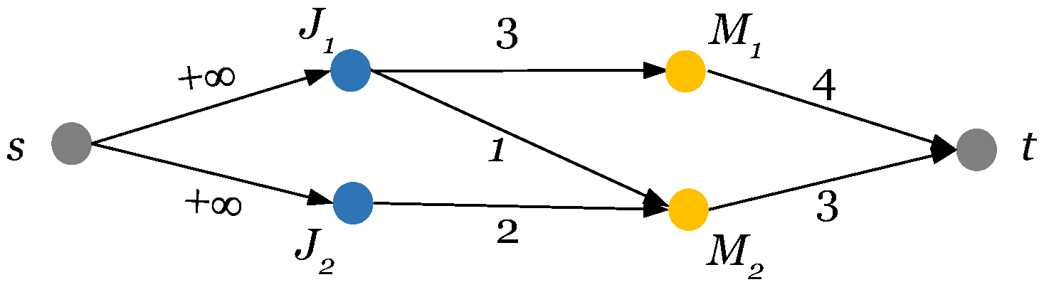
Transforming DLF means that we should build a flow network that could well model jobs, sites, capacity constraint, rational constraint, and the integral requirements. Before giving a formal description, we perform a concrete case study first. Consider there are two jobs $J_1$, $J_2$ executed over two sites $M_1$, $M_2$. The demands of the two jobs are respectively $\langle 3,1\rangle$ and $\langle 0,2\rangle$, while the capacity of $M_1$ is 4 and the capacity of $M_2$ is 3. Figure 1 depicts the flow network built for the case. We can see that $J_1$, $J_2$ and $M_1$, $M_2$ all appear as nodes in the graph. We use directly edges between jobs and sites to express the demands (by edge capacity). s and t in the graph represent respectively the source and sink node which are essential for any flow network. We add directed edges between s and the two jobs, where the capacity has no special constraint (expressed by $+\infty$). We also add directed edges from every site to t, where the capacity of edge is set to the corresponding capacity of site. Our general idea is to use the amount of flow passing by $J_1$ and $J_2$ to model the corresponding allocations. It is well-known that a feasible flow never breaks the capacity of any edge in the flow network. With the above settings, any feasible flow satisfies the capacity and rational constraints. If we further require that the flow is in integral field (i.e., for any feasible flow, the amount of flow on any edge is an integer), a feasible allocation actually corresponds to a feasible flow and vice versa.

Now let us give a formal description on problem transformation. Necessary notations are introduced first. We consider graph $G=(V,E)$ with a capacity function $c:E\to {\mathbb{Z}}^{+}$, where $V=\left\{s\right\}\cup \mathcal{J}\cup \mathcal{M}\cup \left\{t\right\}$. s and t represent the source node and the sink node, respectively, in a flow network. $\mathcal{J}$ is the set of nodes representing jobs and $\mathcal{M}$ is the set of nodes corresponding to sites. Each edge $e\in E$ is denoted as a pair of ordered nodes, i.e., $e=\langle v_p,v_q\rangle$. The capacity function c is defined in the following.

$$\begin{array}{cc}\hfill c(e)& =\left\{\begin{array}{cc}{d}_{ij}\hfill & \mathrm{if}{v}_p=J_i\mathrm{and}{v}_q=M_j;\hfill \\ +\infty \hfill & \mathrm{if}{v}_p=s\mathrm{and}{v}_q=J_i;\hfill \\ C_j\hfill & \mathrm{if}{v}_p=M_j\mathrm{and}{v}_q=t;\hfill \\ 0\hfill & \mathrm{otherwise}.\hfill \end{array}\right.\hfill \end{array}$$

(4)

By removing the edges that have an empty capacity, the flow network graph that we obtained for problem transformation is given in Figure 2.

In the flow network constructed, we can also provide a formal definition on feasibility. A flow f on G is called feasible if it satisfies two conditions that the amount of flow over any edge $e\in E$ is a positive integer $f(e)\in {\mathbb{Z}}^{+}$ and never exceeds the capacity $f(e)\le c(e)$. For ease of representation, we use $\left|f\right|$ to express the total amount flow of f. Clearly, $\left|f\right|={\sum }_{e\in E}f(e)$ is an integer too. Based on $f(e)\le c(e)$, we have two inequalities given below:

$$\forall \langle M_j,t\rangle \in E,\sum _{i=1}^{n}f(\langle J_i,M_j\rangle )\le c(\langle M_j,t\rangle )=C_j,$$

(5)

$$\forall J_i\in V,M_j\in V,0\le f(\langle J_i,M_j\rangle )\le d_{ij}.$$

(6)

By considering $f(\langle J_i,M_j\rangle )$ as $a_{ij}$, it is easy to verify that the above inequalities actually refer to the feasible and rational allocation constraints, respectively. Consequently, a feasible flow f on G corresponds to a feasible resource allocation ${\mathbf{A}}_{n\times m}$, and vice versa. For each job $J_i$, its aggregate resource allocation is the amount of flow passing by node $J_i$ in graph G:

$$\forall M_j\in V,{\overrightarrow{A}}_i=f(\langle s,J_i\rangle )=\sum _{j}f(\langle J_i,M_j\rangle )=\sum _j{a}_{ij}.$$

(7)

To avoid redundant notations, we also write $f\in \mathcal{X}$ to mean f is feasible and let $\varphi (f)=\varphi (\overrightarrow{A})$ be the corresponding nondecreasing order. A DLF allocation corresponds to a lexicographically optimal flow whose definition is given below.

Definition 4.

A flow $f\in \mathcal{X}$ is lexicographically optimal if and only if $\forall f^{\prime }\in \mathcal{X}$ there is $\varphi (f^{\prime })\le \varphi (f)$.

4. Basic Properties

In network flow theory, maximum flow is a well-known problem [14]. One of the classic theorems is the augmenting path theorem [15,16], which plays an important role in many related algorithms [17]. A well-known property is that maximum flow algorithm is also suitable for the integral setting where the amount of flow can only be formulated by an integer. N. Megiddo [18,19] studied multisource and multisink lexicographically optimal flow, the algorithm proposed in [19] is a natural extension of Dinic maximum flow algorithm [20]. In our paper, we also leverage maximum flow theories to carry out the key proofs. Note that if $f\in \mathcal{X}$ is maximal then $\forall f^{\prime }\in \mathcal{X}$, there is $|f^{\prime }|\le |f|$.

Lemma 1.

If f is a maximal flow on G, then $\forall M_j\in V$, ${\sum }_{i}f(\langle J_i,M_j\rangle )=min(C_j,{\sum }_i{d}_{ij})$.

By combining (5) and (6), we have ${\sum }_{i}f(\langle J_i,M_j\rangle )\le min(C_j,{\sum }_i{d}_{ij})$. If the inequality is strictly satisfied, there must exist two successive edges $\langle J_{i^{\prime }},M_j\rangle$ and $\langle M_j,t\rangle$ such that $f(\langle J_{i^{\prime }},M_j\rangle )<d_{i^{\prime }j}$ and ${\sum }_{i}f(\langle J_{i^{\prime }},M_j\rangle )<C_j$. Clearly, $\left|f\right|$ can be increased, which contradicts with f being maximal.

In our model, if a flow $f\in \mathcal{X}$ is lexicographically optimal, it is easy to verify that f is also a maximal flow but not vice versa, i.e., a lexicographically optimal flow is a special maximal flow. Given a feasible flow f on G, an augmenting path is a directed simple path from s to t (e.g., $\mathbb{P}=\{s,v_1,v_2,...,v_i,v_{i+1},...,t\}$) on the residual graph $G_f$. Similarly, an adjusting cycle $\mathbb{C}$ on $G_f$ is a directed simple cycle from s to s (does not pass by t). The capacity of a given path (or a given cycle) is defined to be the capacity of the corresponding bottleneck edge, e.g., for a path $\mathbb{P}$, $c(\mathbb{P})={min}_{e=\langle v_i,v_{i+1}\rangle \in \mathbb{P}}c(e)$ and for a cycle $\mathbb{C}$, $c(\mathbb{C})={min}_{e=\langle v_i,v_{i+1}\rangle \in \mathbb{C}}c(e)$. For ease of representation, we consider augmenting path or adjusting cycle to only contain edges with positive capacity, i.e., $c(\mathbb{P})>0$ and $c(\mathbb{C})>0$.

In our context, performing an augmentation means increasing the original flow f by $\delta$ ($\delta \in {\mathbb{Z}}^{+}$ and $1\le \delta \le c(\mathbb{P})$) along an augmenting path $\mathbb{P}$ in $G_f$ and performing an adjustment means adjusting the original flow f by $\delta$ ($\delta \in {\mathbb{Z}}^{+}$ and $1\le \delta \le c(\mathbb{C})$) along an adjusting cycle $\mathbb{C}$ in $G_f$. By performing an augmentation or an adjustment on a flow f, we can get a new feasible flow. The difference is that only the augmentation increases $\left|f\right|$.

Claim 1.

For a given feasible flow f on G, if there does not exist any augmenting path passing by $J_k$ in $G_f$, then for any feasible $f^{\prime }$ augmented from f, there is also no augmenting path passing by $J_k$ in $G_{f^{\prime }}$.

Proof. 

We prove by contradiction: assume there exists a feasible flow $f^{\prime }$ augmented from f and in the residual graph $G_{f^{\prime }}$, however, there is an augmenting path passing by $J_k$ (denoted by ${\mathbb{P}}^{*}$ in the following). In our model, $c(\langle s,J_k\rangle )=+\infty$, which implies $\langle s,J_k\rangle$ is an edge existing in any residual graph. Therefore, we only need to consider ${\mathbb{P}}^{*}$ where the first two nodes are s and $J_k$.

As $f^{\prime }$ is augmented from f, we can perform successive augmentations on f to get $f^{\prime }$. Note that each augmentation is performed along an augmenting path. Hence, assume the successive augmentations are performed on a sequence of augmenting paths $\mathcal{P}=\{{\mathbb{P}}_1,{\mathbb{P}}_2,...,{\mathbb{P}}_r\}$ which are respectively in the intermediate residual graphs $\{G_1,G_2,...,G_r\}$ obtained by augmentations. Here $G_1$ is exactly $G_f$, $G_2$ is obtained by perform an augmentation along ${\mathbb{P}}_1$ on $G_1$, et al. Next, we perform a recursive analysis to gradually reduce $\mathcal{P}$ and finally prove that in $G_f$ there also exists an augmenting path passing by $J_k$, which leads to a contradiction.

Finding ${\mathbb{P}}_{\ell }$ the last path in $\mathcal{P}$ which has common nodes (except s, $J_k$ and t) with ${\mathbb{P}}^{*}$: ${\mathbb{P}}_{\ell }\cap {\mathbb{P}}^{*}/\{s,J_k,t\}\ne \varnothing$. A special case is that we cannot find such ${\mathbb{P}}_{\ell }$. It means that starting from $G_f$ by performing augmentations along all the augmenting paths in $\mathcal{P}$, there is no influence on the existence of ${\mathbb{P}}^{*}$, i.e., ${\mathbb{P}}^{*}$ is already an augmenting path in $G_f$.

If such ${\mathbb{P}}_{\ell }$ exists, it implies that after the augmentation is performed along ${\mathbb{P}}_{\ell }$ in $G_{\ell }$, the follow-up augmentations along ${\mathbb{P}}_{\ell +1}$, ${\mathbb{P}}_{\ell +2}$, …, ${\mathbb{P}}_r$ do not affect the existence of ${\mathbb{P}}^{*}$ any more, i.e., ${\mathbb{P}}^{*}$ exists in $G_{\ell +1}$, $G_{\ell +2}$, …, $G_r$. Now let us focus on finding an augmentation path passing by $J_k$ which appears in $G_{\ell }$ (before the augmentation along ${\mathbb{P}}_{\ell }$ is performed). Assume $v_x$ is the first node not only passing by ${\mathbb{P}}_{\ell }$ but also appearing in ${\mathbb{P}}^{*}$. We know that the augmentation along ${\mathbb{P}}_{\ell }$ does not affect the existence of the first part of ${\mathbb{P}}^{*}$: $\{s,J_k,...,v_x\}$. The remaining part of ${\mathbb{P}}^{*}$ may not exist in $G_{\ell }$. However, we can replace it with the part $\{v_x,...,t\}$ that appears in ${\mathbb{P}}_{\ell }$. By concatenating the above two parts together, we actually find another augmentation path in $G_{\ell }$ passing by $J_k$. If ${\mathbb{P}}_{\ell }$ is exactly ${\mathbb{P}}_1$ of $\mathcal{P}$, we already find an augmentation path passing by $J_k$ in $G_f$. Otherwise, let us denote the new found augmentation path by ${\mathbb{P}}^{*}$ too, reduce $\mathcal{P}$ to $\{{\mathbb{P}}_1,{\mathbb{P}}_2,...,{\mathbb{P}}_{\ell }\}$ and restart the whole process. As $\mathcal{P}$ is not infinite, the process will be stopped after finite times, which implies $G_f$ must include an augmentation path passing by $J_k$. □

In our model, if a maximal flow is also lexicographically optimal, it must satisfy a special condition. In a residual graph $G_f$, we name a simple path is a $J_p\to J_q$ path if it starts at $J_p$, ends at $J_q$, and does not pass by s and t. Note that any $J_p\to J_q$ path only contains edges with positive capacity.

Theorem 2.

A maximal flow f on G is lexicographically optimal if and only if for all $J_p$ and $J_q$, if ${\overrightarrow{A}}_p\le {\overrightarrow{A}}_q-2$, then there is no $J_p\to J_q$ path on the residual graph $G_f$.

Proof. 

First, proving the “only if” side. Assume there exist $J_p$ and $J_q$, where ${\overrightarrow{A}}_p\le {\overrightarrow{A}}_q-2$ and a $J_p\to J_q$ path exists in $G_f$. As the existence of $\langle s,J_p\rangle$ and $\langle J_q,s\rangle$, we can perform an adjustment by 1-unit from s to $J_p$, then along the $J_p\to J_q$ path and along the edge $\langle J_q,s\rangle$ to reach s again. Note that by the above adjustment, we obtain a new maximal flow $f^{\prime }$ where ${\overrightarrow{A}}_p^{\prime }={\overrightarrow{A}}_p+1\le {\overrightarrow{A}}_q-1={\overrightarrow{A}}_q^{\prime }$. Therefore, $f^{\prime }$ is lexicographically larger than f, i.e., $\varphi (f^{\prime })>\varphi (f)$, which contradicts with f is lexicographically optimal.

Second, proving the “if” side by contradiction. Suppose that flow f is maximal on G and satisfies the condition. However, it is not lexicographically optimal. Assume $f_{opt}$ is a lexicographically optimal flow such that $\varphi (f_{opt})>\varphi (f)$ and $\left|f\right|=|f_{opt}|$. By comparing f with $f_{opt}$, the set of jobs $\mathcal{J}$ can be naturally divided into three parts ${\mathcal{J}}^{<}=\{J_i\in \mathcal{J}|f(\langle s,J_i\rangle )<f_{opt}(\langle s,J_i\rangle )\}$, ${\mathcal{J}}^{=}=\{J_i\in \mathcal{J}|f(\langle s,J_i\rangle )=f_{opt}(\langle s,J_i\rangle )\}$ and ${\mathcal{J}}^{>}=\{J_i\in \mathcal{J}|f(s,J_i)>f_{opt}(\langle s,J_i\rangle )\}$. Next, we construct a special graph $G_{diff}$ [21] to differentiate $f_{opt}$ and f.

Let us denote $G_{diff}=(V_{diff},E_{diff})$, where $V_{diff}=\mathcal{J}\cup \mathcal{M}$. We also define a capacity function $c_{diff}$ for the edges of $E_{diff}$:

• if $f(\langle J_i,M_j\rangle )\le f_{opt}(\langle J_i,M_j\rangle )$, then $c_{diff}(\langle J_i,M_j\rangle )=f_{opt}(\langle J_i,M_j\rangle )-f(\langle J_i,M_j\rangle )$ and $c_{diff}(\langle M_j,J_i\rangle )=0$;
• otherwise, $c_{diff}(\langle M_j,J_i\rangle )=f(\langle J_i,M_j\rangle )-f_{opt}(\langle J_i,M_j\rangle )$ and $c_{diff}(\langle J_i,M_j\rangle )=0$.

According to Lemma 1, we know for any site $M_j$ there is $f_{opt}(\langle M_j,t\rangle )=f(\langle M_j,t\rangle )$. Therefore, in the graph $G_{diff}$, for each $M_j$, we have ${\sum }_i{c}_{diff}(\langle M_j,J_i\rangle )={\sum }_i{c}_{diff}(\langle J_i,M_j\rangle )$.

In $G_{diff}$, there could exist “positive cycles” (denoted by $\mathbb{C}$): for each edge e of $\mathbb{C}$, there is $c_{diff}(e)>0$. For a positive cycle $\mathbb{C}$, we let $cap$ be the minimum capacity of all the edges contained in $\mathbb{C}$. We shall eliminate all these cycles by capacity reductions. For each edge e of $\mathbb{C}$, we perform $c_{diff}(e)=c_{diff}(e)-cap$. Clearly, after the reduction, $\mathbb{C}$ is no more a positive cycle. Note that once we eliminate a positive cycle $\mathbb{C}$ on $G_{diff}$, it is equivalent to perform an adjustment by $cap$ on $G_f$. For example, assume $J_i$ is a node included in the cycle $\mathbb{C}$. The adjustment is starting from s, along the edge $\langle s,J_i\rangle$, then along the cycle $\mathbb{C}$ back to $J_i$, and finally along the edge $\langle J_i,s\rangle$ back to s. We can eliminate all the positive cycles to get a new $G_{diff}^{\prime }$ by performing a sequence of capacity reduction operations. Compared with $G_{diff}$, $G_{diff}^{\prime }$ corresponds to another maximal flow $f^{\prime }$, where $\forall J_i$, there is $f(s,J_i)=f^{\prime }(s,J_i)$. Hence, $f^{\prime }$ is not lexicographically optimal either. Moreover, ${\mathcal{J}}^{<}$, ${\mathcal{J}}^{=}$ and ${\mathcal{J}}^{>}$ are always kept during the capacity reductions. In the following, we turn to focus on $G_{diff}^{\prime }$.

In $G_{diff}^{\prime }$, there must exist positive paths (for each edge in the path, the capacity is a positive integer), otherwise the flow $f^{\prime }$ is exactly $f_{opt}$, which implies both f and $f^{\prime }$ are also lexicographically optimal. As there are no positive cycles in $G_{diff}^{\prime }$, we can extend any positive paths to be a maximal positive path, where there are no edges with positive capacity entering the starting point and no edges with positive capacity leaving the ending point. The minimum capacity of edges in a maximal positive path is also denoted by $cap\ge 1$. Next, we shall demonstrate that for any maximal positive path in $G_{diff}^{\prime }$, the starting point $J_p$ must belong to ${\mathcal{J}}^{<}$ and the ending point $J_q$ must belong to ${\mathcal{J}}^{>}$. Clearly, $J_p$ cannot belong to ${\mathcal{J}}^{>}$ due to every node in ${\mathcal{J}}^{>}$ having positive entering edges. On the other hand, $J_p$ cannot belong to ${\mathcal{J}}^{=}$ nor $\mathcal{M}$, since for each node in ${\mathcal{J}}^{=}$ or in $\mathcal{M}$, the total capacity of the positive entering edges is equal to the total capacity of the positive leaving edges. Consequently, $J_p$ can only belong to ${\mathcal{J}}^{<}$. Similarly, we can infer that the ending point $J_q$ can only belong to ${\mathcal{J}}^{>}$. Now we show that the maximal positive path in $G_{diff}^{\prime }$ corresponds to a $J_p\to J_q$ path in $G_f$. First, note that from $G_{diff}$ to $G_{diff}^{\prime }$, we only decrease the capacity of some edges, such that if a maximal positive path appears in $G_{diff}^{\prime }$, it is also a path in $G_{diff}$ (not necessarily maximal).

Suppose $\langle J_i,M_j\rangle$ is a directed edge in the maximal positive path. $\langle J_i,M_j\rangle$ is also an edge having positive capacity in $G_{diff}$. Then, $c_f(\langle J_i,M_j\rangle )$ the capacity of the edge $\langle J_i,M_j\rangle$ inside $G_f$ satisfies:

$$c_f(\langle J_i,M_j\rangle )=c(\langle J_i,M_j\rangle )-f(\langle J_i,M_j\rangle )\ge max(f_{opt}(\langle J_i,M_j\rangle )-f(\langle J_i,M_j\rangle ),0)=c_{diff}(\langle J_i,M_j\rangle )$$

Similarly, assume $\langle M_j,J_i\rangle$ is a directed edge in the maximal positive path. $\langle M_j,J_i\rangle$ is also an edge with positive capacity in $G_{diff}$. $c_f(\langle M_j,J_i\rangle )$ the capacity of the edge $\langle M_j,J_i\rangle$ inside $G_f$ satisfies:

$$c_f(\langle M_j,J_i\rangle )=f(\langle J_i,M_j\rangle )\ge max(f(\langle J_i,M_j\rangle )-f_{opt}(\langle J_i,M_j\rangle ),0)=c_{diff}(\langle M_j,J_i\rangle )$$

The above two formulas together indicate that for each edge of a maximal positive path in $G_{diff}$, the capacity of the corresponding edge in $G_f$ is also positive. Without loss of generality, assume a maximal positive path that starts at $J_p$ and ends at $J_q$. Then we get the corresponding $J_p\to J_q$ path in $G_f$. According to the assumption on f, we can easily infer that ${\overrightarrow{A}}_p\ge {\overrightarrow{A}}_q-1$ as the existence of the $J_p\to J_q$ path. Next, we show that f must be lexicographically optimal.

First, let us assume ${\overrightarrow{A}}_p\ge {\overrightarrow{A}}_q$. Together with the existence of the maximal positive path from $J_p$ to $J_q$, we can infer that ${\overrightarrow{A}}_p^{opt}>{\overrightarrow{A}}_p\ge {\overrightarrow{A}}_q>{\overrightarrow{A}}_q^{opt}$. By considering that the problem is defined in integral field, we can obtain ${\overrightarrow{A}}_p^{opt}\ge {\overrightarrow{A}}_p+1\ge {\overrightarrow{A}}_q+1\ge {\overrightarrow{A}}_q^{opt}+2$. Note that as the maximal path exists, there is a $J_q\to J_p$ path (a reversed path from $J_q$ to $J_p$) in the residual graph $G_{opt}$. As the sufficiency of this theorem is already proven, we can get that ${\overrightarrow{A}}_q^{opt}\ge {\overrightarrow{A}}_p^{opt}-1$. Above all, we can obtain ${\overrightarrow{A}}_p^{opt}\ge {\overrightarrow{A}}_q^{opt}+2\ge {\overrightarrow{A}}_p^{opt}+1$. A contradiction is identified, which means only ${\overrightarrow{A}}_p={\overrightarrow{A}}_q-1$ can happen.

Consider ${\overrightarrow{A}}_p={\overrightarrow{A}}_q-1$. Note that in this case we still have the $J_p\to J_q$ path in $G_f$ and such that ${\overrightarrow{A}}_q^{opt}\ge {\overrightarrow{A}}_p^{opt}-1$. Next, we focus on the maximal positive path from $J_p$ to $J_q$ in $G_{diff}^{\prime }$ and do capacity reductions by $cap$ along such maximal path. Remember that the capacity reductions correspond to do an adjustment in $G_{f^{\prime }}$, which results in a new maximal flow $f^{″}$ that satisfies $|f^{″}|=|f^{\prime }|=|f|$, ${\overrightarrow{A}}_p^{″}={\overrightarrow{A}}_p^{\prime }+cap={\overrightarrow{A}}_p+cap$ and ${\overrightarrow{A}}_q^{″}={\overrightarrow{A}}_q^{\prime }-cap={\overrightarrow{A}}_q-cap$. Together with ${\overrightarrow{A}}_p={\overrightarrow{A}}_q-1$, we have ${\overrightarrow{A}}_p^{″}={\overrightarrow{A}}_q^{″}+2cap-1$. The new difference graph $G_{diff}^{″}$ is obtained by capacity reductions. Hence, in $G_{diff}^{″}$, for node $J_p$ there are no positive edges entering in and for node $J_q$ there are no positive edges leaving out. Therefore, we have ${\overrightarrow{A}}_p^{opt}\ge {\overrightarrow{A}}_p^{″}$ and ${\overrightarrow{A}}_q^{opt}\le {\overrightarrow{A}}_q^{″}$. Above all, we have

$${\overrightarrow{A}}_p^{opt}\ge {\overrightarrow{A}}_p^{″}={\overrightarrow{A}}_q^{″}+2cap-1\ge {\overrightarrow{A}}_q^{opt}+2cap-1\ge {\overrightarrow{A}}_p^{opt}+2cap-2.$$

Let us assume $cap\ge 2$. According to the above inequality, we have ${\overrightarrow{A}}_p^{opt}\ge {\overrightarrow{A}}_p^{opt}+2$, which also results in a contraction.

Now we can conclude that for any maximal path existing in $G_{diff}^{\prime }$ (w.l.o.g, $J_p$ and $J_q$ represents respectively the starting point and the ending point), we must have ${\overrightarrow{A}}_p={\overrightarrow{A}}_q-1$ and $cap=1$. We perform capacity reductions by $cap=1$ along such maximal positive path. The adjustment corresponding to such capacity reductions is to increase ${\overrightarrow{A}}_p$ by 1 and meanwhile to decrease ${\overrightarrow{A}}_q$ by 1. Note that for the flow $f^{″}$ got after the adjustment, there is $\varphi (f^{″})=\varphi (f^{\prime })=\varphi (f)$. It means that the adjustment cannot make f be better in terms of lexicographical order. Finally, we continue to perform capacity reductions along maximal positive paths one by one until no positive edges remains in the difference graph (i.e., $f_{opt}$ is obtained). As no adjustment can make f be better, f is already lexicographically optimal.  □

Corollary 1.

If both f and $f^{\prime }$ are lexicographically optimal, they are interchangeable.

The above corollary is straightforward by the proof of Theorem 2. One can construct the different graph between f and $f^{\prime }$. Then, capacity reductions can be performed to eliminate all positive cycles and maximal positive paths, which is indeed a process of transformation between the two optimal flows.

Lexicographically optimal flow is not unique. Let $LOF$ be the set including all lexicographically optimal flows. Next, we study the variation of aggregate resource obtained by a job among different optimal flows.

Definition 5.

For any $J_i\in \mathcal{J}$, the value interval $I_i$ is defined as the value range of the aggregate resource ${\overrightarrow{A}}_i$ in all $f\in LOF$.

Remember that our problem is discussed in ${\mathbb{Z}}^{+}$ such that each value interval we defined only includes integers. The following theorem shows that the length of any value interval is at most 1.

Theorem 3.

$\forall f,f^{\prime }\in LOF$, $\forall J_i\in \mathcal{J}$, there is $|{\overrightarrow{A}}_i-{\overrightarrow{A}}_i^{\prime }|\le 1$.

Proof. 

We prove by contradiction. Assume there exists a pair of flows $f,f^{\prime }\in LOF$ and there exists a job $J_p\in \mathcal{J}$ which satisfies ${\overrightarrow{A}}_p^{\prime }-{\overrightarrow{A}}_p\ge 2$. Based on the proof of Theorem 2, we construct the difference graph $G_{diff}$ between f and $f^{\prime }$ and target to transform f to $f^{\prime }$. As ${\overrightarrow{A}}_p$ needs to be increased, we have $J_p\in {\mathcal{J}}^{<}$. Moreover, during the transformation, there must exist a time that $J_p$ becomes a starting point of a maximal positive path. Suppose the ending point of such path is $J_q$. We have $J_q\in {\mathcal{J}}^{>}$ (such that ${\overrightarrow{A}}_q>{\overrightarrow{A}}_q^{\prime }$) and ${\overrightarrow{A}}_p={\overrightarrow{A}}_q-1$. On the other hand, the reverse of such maximal path is a $J_q\to J_p$ path on the residual graph $G_{f^{\prime }}$. According to Theorem 2, there is ${\overrightarrow{A}}_q^{\prime }\ge {\overrightarrow{A}}_p^{\prime }-1$. Above all, we can show that ${\overrightarrow{A}}_p^{\prime }\ge {\overrightarrow{A}}_p+2={\overrightarrow{A}}_q+1>{\overrightarrow{A}}_q^{\prime }+1\ge {\overrightarrow{A}}_p^{\prime }$, which is a contradiction as ${\overrightarrow{A}}_p^{\prime }>{\overrightarrow{A}}_p^{\prime }$ is obtained. □

Based on the Theorem 3, we provide a more specified definition of value interval.

Definition 6.

A job $J_i$’s value interval $I_i$ is $[L,L]$ if and only if ${\overrightarrow{A}}_i=L$ for all $f\in LOF$. A job $J_i$’s value interval $I_i$ is $[L,L+1]$ if and only if there exist a pair of flows $f,f^{\prime }\in LOF$ such that ${\overrightarrow{A}}_i=L$ and ${\overrightarrow{A}}_i^{\prime }=L+1$.

Theorem 4.

For a job $J_p\in \mathcal{J}$, suppose ${\overrightarrow{A}}_p=L$ of a given flow $f\in LOF$. $J_p$’s value interval is $[L,L+1]$ if and only if there exists a $J_p\to J_q$ path in the residual graph $G_f$ where ${\overrightarrow{A}}_p={\overrightarrow{A}}_q-1$.

Proof. 

For the “if” side, since one could obtain a new flow $f^{\prime }\in LOF$ by performing an adjustment along the edge $\langle s,J_p\rangle$, then along the $J_p\to J_q$ path and along the edge $\langle J_q,s\rangle$ back to s. In the new flow $f^{\prime }$, there is ${\overrightarrow{A}}_p^{\prime }=L+1$, which implies $I_p=[L,L+1]$.

For the “only if” side, there exists a flow $f^{\prime }\in LOF$ with ${\overrightarrow{A}}_p^{\prime }=L+1$. Based on the proof of Theorem 2, we transform f to $f^{\prime }$. We first eliminate all positive cycles and then eliminate maximal positive path one by one. During the transformation process, we can find a maximal positive path which starts at $J_p$ and ends at another node $J_q$ satisfying ${\overrightarrow{A}}_p={\overrightarrow{A}}_q-1$. By such maximal path, we can identify the corresponding $J_p\to J_q$ path on $G_f$. □

By Theorem 4, we directly have the following two corollaries.

Corollary 2.

For a job $J_p\in \mathcal{J}$, suppose ${\overrightarrow{A}}_p=L$ under a given flow $f\in LOF$. $J_p$’s value interval is $[L-1,L]$ if and only if there exists a $J_q\to J_p$ path in the residual graph $G_f$ where ${\overrightarrow{A}}_q={\overrightarrow{A}}_p-1$.

Corollary 3.

For a job $J_p\in \mathcal{J}$, suppose ${\overrightarrow{A}}_p=L$ under a given flow $f\in LOF$. $J_p$’s value interval is $[L,L]$ if and only if in the residual graph $G_f$ there neither exists a $J_p\to J_q$ path where ${\overrightarrow{A}}_p={\overrightarrow{A}}_q-1$ nor exists a $J_q\to J_p$ path where ${\overrightarrow{A}}_q={\overrightarrow{A}}_p-1$.

We define binary relations on value intervals in order to make the comparison. Let $I_p=[L_p,R_p]$ and $I_q=[L_q,R_q]$ be the two value intervals of $J_p$ and $J_q$ respectively. $I_p<I_q$ if and only if $L_p<L_q$ or $R_p<R_q$. Symmetrically, $I_p>I_q$ if and only if $L_p>L_q$ or $R_p>R_q$. Finally, $I_p=I_q$ if and only if $L_p=L_q$ and $R_p=R_q$.

Theorem 5.

Suppose $f\in LOF$ and in the residual graph $G_f$ there exists a $J_p\to J_q$ path where ${\overrightarrow{A}}_p={\overrightarrow{A}}_q-1=L$. Let $\mathbb{P}$ denote the set of jobs passed by the $J_p\to J_q$ path, then $\forall J_k\in \mathbb{P}$, there is $I_k=[L,L+1]$.

Proof. 

The value intervals of $J_p$ and $J_q$ can be obtained directly by Theorem 4 and Corollary 2, respectively. Both of them are equal to $[L,L+1]$. Suppose $J_k\in \mathbb{P}$ and $J_k$ is not $J_p$ nor $J_q$. Clearly, we have a $J_p\to J_k$ path and a $J_k\to J_q$ path in the residual graph $G_f$. Assume $J_k$’s value interval $I_k\le [L-1,L]$, i.e., $\overrightarrow{A_k}\le L-1$ under the current flow f. Then we can perform an adjustment by 1 along the edge $\langle s,J_k\rangle$, then along the $J_k\to J_q$ path and along the edge $\langle J_k,s\rangle$ back to s. After the adjustment, we obtain a new flow $f^{\prime }$, where ${\overrightarrow{A_k}}^{\prime }=L$ and ${\overrightarrow{A_q}}^{\prime }=L$. However, it implies that $f^{\prime }$ satisfies $\varphi (f^{\prime })>\varphi (f)$ which contradicts with f is lexicographically optimal. Symmetrically, we can prove that $I_k\ge [L,L+1]$ is not true too due to the existence of the $J_p\to J_k$ path in $G_f$. Above all, we can conclude $I_k=[L,L+1]$. □

Definition 7.

A feasible flow f on G is lexicographically feasible if and only if $\forall J_p,J_q\in \mathcal{J}$, if ${\overrightarrow{A}}_p\le {\overrightarrow{A}}_q-2$, then no $J_p\to J_q$ path exists in the residual graph $G_f$.

Definition 8.

A lexicographically feasible flow f on G is called v-strict if and only if $\forall J_i\in \mathcal{J}$, there is ${\overrightarrow{A}}_i\le v$ and if ${\overrightarrow{A}}_i\le v-1$, then in $G_f$ there is no augmenting path passing by $J_i$.

For any given lexicographically optimal flow, we can get one unique value:

$$v_{max}=max\{{\overrightarrow{A}}_1,{\overrightarrow{A}}_2,...,{\overrightarrow{A}}_n\}.$$

From Definitions 7 and 8, we can easily see that a lexicographically optimal flow is $v_{max}$-strict. Additionally, we consider the empty flow ($\left|f\right|=0$) as 0-strict. Starting from the empty flow, a lexicographically optimal flow could be obtained after a sequence of water-filling stages are carried out.

Definition 9.

A water-filling stage is performed on any v-strict ($0\le v<v_{max}$) flow: performing augmentation by 1 for each job node in the set ${\mathcal{J}}^v=\{J_i\in \mathcal{J}|{\overrightarrow{A}}_i=v\}$.

Note that by a water-filling stage, it is not necessarily that $\forall J_i\in {\mathcal{J}}^v$, ${\overrightarrow{A}}_i$ is increased by 1, as there may already be no augmentation path passing by $J_i$ in $G_f$. According to Claim 1, we know that if ${\overrightarrow{A}}_i$ fails to be increased, then it will no more be increased during the following water-filling stages. That is also the reason that for a v-strict flow a water-filling stage only needs to focus on nodes in ${\mathcal{J}}^v$.

Lemma 6.

A lexicographically optimal flow is obtained after $v_{max}$ water-filling stages.

Proof. 

This lemma is true if during all water-filling stages there is no flow obtained breaks lexicographic feasibility (Definition 7).

Without loss of generality, let us focus on one water-filling stage which will be performed on a v-strict flow, where $0\le v<v_{max}$. In such stage, we know there are a sequence of augmentations that will be performed for each node in the set ${\mathcal{J}}^v$. Clearly, before any augmentations are performed, the v-strict flow is lexicographically feasible. We need to prove that after any augmentation is successfully performed, the new flow obtained is still lexicographically feasible.

Suppose after a sequence augmentations the flow f obtained is still lexicographically feasible. In the current state, we can divide jobs into three parts: $S_1=\{J_i\in \mathcal{J}|{\overrightarrow{A}}_i\le L-1\}$, $S_2=\{J_i\in \mathcal{J}|{\overrightarrow{A}}_i=L\}$ and $S_3=\{J_i\in \mathcal{J}|{\overrightarrow{A}}_i=L+1\}$. Consider that the next augmentation will be executed along an augmenting path (denoted by $\mathbb{P}$) that passes by node $J_k$ and assume that after the augmentation the new flow $f^{\prime }$ is not lexicographically feasible, i.e., in $G_f^{\prime }$, there exists a $J_p\to J_q$ path where ${\overrightarrow{A}}_p\le {\overrightarrow{A}}_q-2$. Since $L+1=max\{{\overrightarrow{A}}_1,{\overrightarrow{A}}_2,...,{\overrightarrow{A}}_n\}$, we have $J_p\in S_1$ which implies ${\overrightarrow{A}}_p$ will not be increased during the current water-filling stage. There are two cases. First, in $G_f^{\prime }$, $\mathbb{P}$ and the $J_p\to J_q$ path have no intersections (share common nodes in the path). In this case, we can infer that the $J_p\to J_q$ path also exists in $G_f$, as the augmentation does not affect the existence of the $J_p\to J_q$ path. On the other hand, we can infer that under the flow f there is also ${\overrightarrow{A}}_p\le {\overrightarrow{A}}_q-2$. The reason is that from f to $f^{\prime }$ both ${\overrightarrow{A}}_p$ and ${\overrightarrow{A}}_q$ are kept. However, it violates the assumption that f is lexicographically feasible. Second, in $G_f^{\prime }$, $\mathbb{P}$ and the $J_p\to J_q$ path have intersections. Along the two paths, let us assume node x is the first common node where the two paths intersect. Note that the sub-path (from $J_p$ to x) of $J_p\to J_q$ is not affected by the augmentation such that it also exists in $G_f$. On the other hand, $\mathbb{P}$ has a sub-path from x to t in $G_f$. Therefore, we can find an augmenting path from s to $J_p$, then from $J_p$ to x and finally from x to t. However, it violates f is v-strict. Above all, we get the proof. □

Theorem 7.

Suppose $J_p$’s value interval is $I_p=\left[L-1,L\right]$. Under any L-strict flow f, if ${\overrightarrow{A}}_p=L-1$, then there exists a $J_p\to J_q$ path on $G_f$ where ${\overrightarrow{A}}_q=L$. Symmetrically, if ${\overrightarrow{A}}_p=L$, then there exists a $J_q\to J_p$ path on $G_f$ where ${\overrightarrow{A}}_q=L-1$.

Proof. 

Since f is L-strict, we can perform a sequence of water-filling stages on f to get a lexicographically optimal flow $f^{\prime }$. Clearly, ${\overrightarrow{A}}_p$ is no more increased during the following water-filling stages such that ${\overrightarrow{A}}_p^{\prime }={\overrightarrow{A}}_p$. First, consider currently ${\overrightarrow{A}}_p=L-1$. According to Corollary 2, we know in $G_{f^{\prime }}$ there exists a $J_p\to J_q$ path where ${\overrightarrow{A}}_q={\overrightarrow{A}}_p+1=L$. Next, we prove that the $J_p\to J_q$ path existing in $G_{f^{\prime }}$ also appears in $G_f$. From f to $f^{\prime }$, successive water-filling stages on f are performed. Every water-filling stage is composed of a sequence of augmentations each of which corresponds to an augmenting path. Thus, we could use an ordered set $\mathcal{S}=\{{\mathbb{P}}_1,{\mathbb{P}}_2,\dots ,{\mathbb{P}}_r\}$ to include all augmenting paths (of all water-filling stages) used for augmenting f to $f^{\prime }$. Suppose ${\mathbb{P}}_i\in \mathcal{S}$ is the last element in $\mathcal{S}$ which shares common nodes with the $J_p\to J_q$ path and suppose the first common node of the two paths is $J_k$. Let $f^{i-1}$ denote the flow before the augmentation along ${\mathbb{P}}_i$ is processed. Note that $f^{i-1}$ is lexicographically feasible according to the proof of Lemma 6. We can infer that the $J_p\to J_k$ path (sub-path of $J_p\to J_q$) already appears in $G_{f^{i-1}}$. On the other hand, there is a path from $J_k$ to t in $G_{f^{i-1}}$, which is the sub-path of ${\mathbb{P}}_i$. Together with the edge $\langle s,J_p\rangle$, we find an augmenting path passing by $J_p$ in $G_{f^{i-1}}$. Remember that f is L-strict such that in $G_f$ there is no augmenting path passing by $J_p$. By Claim 1, we know that in $G_{f^{i-1}}$ there should also be no augmenting path passing by $J_p$, i.e., a contradiction is identified. Therefore, for any path ${\mathbb{P}}_i\in \mathcal{S}$, it shares no common nodes with the $J_p\to J_q$ path, which implies the $J_p\to J_q$ path also exists in $G_f$. The proof for the second case ${\overrightarrow{A}}_p=L$ is symmetric where we can find an augmenting path passing by $J_q$ (with ${\overrightarrow{A}}_q=L-1$) in an intermediately obtained residual graph, which also concludes a contradiction. □

Corollary 4.

For any L-strict flow f on G, if there exists a $J_p\to J_q$ path in $G_f$ where ${\overrightarrow{A}}_p={\overrightarrow{A}}_q-1=L-1$, then the same path also exists in any lexicographically optimal flow $f^{\prime }$ that could be augmented from f.

Corollary 4 is actually the inverse proposition of Theorem 7. The proof can be obtained by applying the proof of Theorem 7 in a reversed direction.

5. Economic Properties

In this section, we investigate whether or not a DLF allocation (or, equivalently, a lexicographically optimal flow) satisfies economic properties which is critical to verifying whether DLF is reasonable to define fairness in our scenario.

5.1. Pareto Efficiency and Envy-Freeness

Pareto efficiency: Increasing the allocation of a job must decrease the allocation of another job.

If Pareto efficiency is satisfied, all the available resources must be allocated or the total resource requirements are already fully met, i.e., resource utilization is maximized. Note that fairness is only necessary when resources cannot meet all the demands. Therefore, any reasonable scheme on fairness should be Pareto efficiency.

Theorem 8.

Distributed lexicographical fairness satisfies Pareto efficiency.

Proof. 

The proof is straightforward. Suppose DLF does not satisfy Pareto efficiency. We know that a DLF allocation corresponds to a lexicographically optimal flow. DLF does not satisfy Pareto efficiency which directly implies that lexicographically optimal flow is not maximal. This is a contradiction.  □

Envy-freeness: no job would expect to get the allocation of any other job.

Envy-freeness is also a usual requirement of any fair scheme. Under a fair allocation, we can easily imagine that no job prefers the allocation of another job. In our setting, envy-freeness could be represented by the following inequality.

$$\forall J_q\in \mathcal{J},\sum _{j}min(a_{qj},d_{pj})\le \sum _j{a}_{pj}.$$

(8)

At first glance, DLF allocation does not always satisfy envy-freeness. For example, there are two jobs, $J_1$ and $J_2$, each of which has one task to be executed on the same site $M_1$ whose time slots is 1. No matter which job gets the time slot, the other one would envy its allocation. This happens due to our discussion area being in ${\mathbb{Z}}^{+}$. Indeed in our setting, $J_p$ never envies $J_q$’s allocation if ${\overrightarrow{A}}_p\le {\overrightarrow{A}}_q-2$.

Theorem 9.

$\forall J_p,J_q\in \mathcal{J}$, if ${\overrightarrow{A}}_p\le {\overrightarrow{A}}_q-2$, then $J_p$ does not envy $J_q$’s allocation.

Proof. 

Proof by contradiction. Suppose f is lexicographically optimal. However, there exists a pair of jobs—$J_p$ and $J_q$, where ${\overrightarrow{A}}_p\le {\overrightarrow{A}}_q-2$ and ${\sum }_{j}min(a_{qj},d_{pj})>{\sum }_j{a}_{pj}$. We can infer that $\exists M_j\in \mathcal{M}$ such that $min(a_{qj},d_{pj})>a_{pj}$. Note that in $G_f$ the two edges $\langle J_p,M_j\rangle$ and $\langle M_j,J_q\rangle$ together form a $J_p\to J_q$ path. Combining with ${\overrightarrow{A}}_p\le {\overrightarrow{A}}_q-2$, we find that a contradiction with f is lexicographically optimal. □

5.2. Strategy-Proofness

Strategy-proofness: No job can get more allocation by lying about its demands.

Strategy-proofness ensures incentive compatibility. This property is important for a fairness scheme. With strategy-proofness, no participant can break the fairness scheme with its own information. In our setting, strategy-proofness is used to ensure that a job should not get profits by misreporting its demands. Suppose $J_{\ell }$ lies about its demands. The demand matrix is denoted by ${\mathbf{D}}_{n\times m}^{\prime }$. Note that under ${\mathbf{D}}_{n\times m}^{\prime }$ we could still compute lexicographically optimal allocation and model the problem under another flow graph denoted by $G^{\prime }$.

Since only $J_{\ell }$ lies, $\forall M_j\in \mathcal{M}$, if $J_k\in \mathcal{J}\backslash \left\{J_{\ell }\right\}$, then $d_{kj}^{\prime }=d_{kj}$. For $J_{\ell }$, we consider $d_{\ell j}^{\prime }$ could be any non-negative integer, i.e., we do not assume $d_{\ell j}^{\prime }\ge d_{\ell j}$. Under the setting with misreporting, the allocation matrix is denoted by ${\mathbf{A}}^{\prime }$. When ${\mathbf{A}}^{\prime }$ is distributed lexicographically fairly, the corresponding lexicographically optimal flow is denoted by $f^{\prime }\in DL{F}^{\prime }$, where $DL{F}^{\prime }$ is the set of lexicographically optimal flows obtained under ${\mathbf{D}}_{n\times m}^{\prime }$.

With mis-reporting, it is easy to verify that for each job $J_i$ the value interval $I_i^{\prime }$ is still in the form $[L,L]$ or $[L,L+1]$ where L is a non-negative integer. For each job $J_i$, we also define its useful allocation to be ${\sum }_{j}min\{d_{ij},a_{ij}^{\prime }\}$, where the minimum is taken to ensure that the actual executed tasks of $J_i$ on any site would not exceed the true demands. Note that if $J_i$ is honest, then ${\sum }_{j}min\{d_{ij},a_{ij}^{\prime }\}={\sum }_j{a}_{ij}^{\prime }$. For simplifying the representation, we let $\overrightarrow{U}$ be the vector of useful aggregate allocation under mis-reporting.

$$\overrightarrow{U}=\langle \sum _{j}min\{d_{1j},a_{1j}^{\prime }\},\sum _{j}min\{d_{2j},a_{2j}^{\prime }\},\dots ,\sum _{j}min\{d_{nj},a_{nj}^{\prime }\}\rangle$$

We define a similar notion called useful value interval ($I^u$), where $I_k^u$ represents the useful value interval covered by the values of ${\overrightarrow{U}}_k$ corresponding to lexicographically optimal flows in $DL{F}^{\prime }$. It can be verified that $I_{\ell }^u\le I_{\ell }^{\prime }$ and for all honest jobs $J_k\in \mathcal{J}\backslash \left\{J_{\ell }\right\}$ there is $I_k^u=I_k^{\prime }$.

Lemma 10.

For the lying job $J_{\ell }$, the length of useful value interval $I_{\ell }^u$ could be larger than 1, i.e., $I_{\ell }^u=[L_{\ell },R_{\ell }]$ s.t. $R_{\ell }$ could be larger than $L_{\ell }+1$.

Proof. 

This lemma can be easily verified by a concrete instance. Consider that there are two jobs $J_1,J_2$ and two sites $M_1,M_2$. Suppose $J_1$ is the job whose will misreport the demand. The genuine and lying demand matrix are given as follows:

$${\mathbf{D}}_{n\times m}=\left(\begin{array}{cc}3& 0\\ 3& 3\end{array}\right){\mathbf{D}}_{n\times m}^{\prime }=\left(\begin{array}{cc}3& 3\\ 3& 3\end{array}\right)$$

Suppose each site has three time slots to allocate. It is straightforward that each job should obtain three slots in any $f^{\prime }\in DL{F}^{\prime }$. All possible allocations are in the following:

$${\mathbf{A}}_{n\times m}^{\prime }=\left(\begin{array}{cc}0& 3\\ 3& 0\end{array}\right){\mathbf{A}}_{n\times m}^{\prime }=\left(\begin{array}{cc}1& 2\\ 2& 1\end{array}\right){\mathbf{A}}_{n\times m}^{\prime }=\left(\begin{array}{cc}2& 1\\ 1& 2\end{array}\right){\mathbf{A}}_{n\times m}^{\prime }=\left(\begin{array}{cc}3& 0\\ 0& 3\end{array}\right)$$

Clearly, in the above example, there is $I_1^u=[0,3]$ showing that $R_{\ell }$ could be larger than $L_{\ell }+1$. □

From the above example, we can also see that $I_1^u$ is continuous, i.e., ${\overrightarrow{U}}_1$ could be any integer in the set $\{0,1,2,3\}$. Actually, the useful value interval of the lying job is always continuous.

Lemma 11.

The useful value interval $I_{\ell }^u$ of the lying job $J_{\ell }$ is continuous.

Proof. 

Select arbitrarily two flows $f_1^{\prime },f_2^{\prime }\in DL{F}^{\prime }$ and suppose the useful allocation of the lying job $J_{\ell }$ is ${\overrightarrow{U}}_k^1$ and ${\overrightarrow{U}}_k^2$, respectively. Without loss of generality, consider ${\overrightarrow{U}}_{\ell }^1\le {\overrightarrow{U}}_{\ell }^2-2$. As $f_1^{\prime }$ and $f_2^{\prime }$ are lexicographically optimal, we know they are interchangeable (Corollary 1). Note that during the process of transforming $f_1^{\prime }$ to $f_2^{\prime }$ (which also increases ${\overrightarrow{U}}_{\ell }^1$ to ${\overrightarrow{U}}_{\ell }^2$), if we can control the amount variation of ${\overrightarrow{U}}_k^1$ upper bounded by “1 unit”, then all middle points (integers) between ${\overrightarrow{U}}_{\ell }^1$ and ${\overrightarrow{U}}_{\ell }^2$ must be obtained (corresponding to a flow obtained during the transformation).

Similar to the proof of Theorem 2, let us construct the graph $G_{diff}$ to depict the difference between $f_1^{\prime }$ and $f_2^{\prime }$, and then eliminate all positive cycles and maximal positive paths. Different from the proof of Theorem 2, here we control the amount of the variation by “1 unit”. For example, if $\mathbb{C}$ is a positive cycle, then only “1 unit” reduction is performed each time: for each edge e of $\mathbb{C}$, do $c_{diff}(e)=c_{diff}(e)-1$. Similarly, each time the amount of reduction during any maximal positive path is also controlled by 1. Now let us consider the variation of ${\overrightarrow{U}}_{\ell }^1$ after a reduction is performed. There are two cases. First, $J_{\ell }$ is included by a positive cycle or located in the middle of a maximal positive path. In this case, $J_{\ell }$ must be adjacent with two site nodes. Without loss of generality, suppose $M_i$ is the in-neighbor and $M_j$ is the out-neighbor. The “1 unit” reduction corresponds to lose one unit resource from $M_i$ and obtain one more unit resource from $M_j$. Second, $J_{\ell }$ is the starting point or the ending point of a maximal positive path. In this case, the allocation of $J_{\ell }$ could be increased by 1 (corresponding to $J_{\ell }$ is the starting point) or be decreased by 1 (corresponding to $J_{\ell }$ is the ending point). It is not difficult to verify that in both cases the variation of the total useful allocation is upper bounded by 1. □

Now we give the definition of strategy-proofness in our setting.

Definition 10.

For distributed lexicographic fairness, strategy-proofness means that no job cannot obtain a larger useful value interval by lying about its demand: if $J_{\ell }$ lies, then there is $I_{\ell }^u\le I_{\ell }$.

Theorem 12.

Distributed lexicographic fairness satisfies strategy-proofness.

Proof. 

For convenience, when there is no misreporting, for each job $J_i\in \mathcal{J}$, we denote the value interval as $I_i=[L_i,R_i]$ and when $J_l$ lies, for each job $J_i\in \mathcal{J}$, we denote the value interval as $I_i^{\prime }=[L_i^{\prime },R_i^{\prime }]$ and denote the useful value interval as $I_i^u=[L_i^u,R_i^u]$. Suppose $J_{\ell }$ is the job which lies. To prove strategy proofness, we need to show that $I_{\ell }^u\le I_{\ell }$ is always true.

In order to prove $I_{\ell }^u\le I_{\ell }$, let us first show that $R_{\ell }^u\le R_{\ell }$. For any lexicographically optimal flow $f^{\prime }$ under misreporting, we could construct a vector called restricted useful allocation as follows:

$$\overrightarrow{T}=\langle min\{{\overrightarrow{U}}_1,{\overrightarrow{U}}_{\ell }\},min\{{\overrightarrow{U}}_2,{\overrightarrow{U}}_{\ell }\},\dots ,min\{{\overrightarrow{U}}_n,{\overrightarrow{U}}_{\ell }\}\rangle$$

Note that $\overrightarrow{T}$ can always be obtained for a given $f^{\prime }$ as $f^{\prime }$ can be obtained by a sequence of water-filling stages which is a reversible procedure. In other words, we can push back flows and remove all $J_x$’s useless resources to get $\overrightarrow{T}$. The flow corresponds to $\overrightarrow{T}$ is called a restricted flow $f^T$. Clearly, $f^T$ is a ${\overrightarrow{U}}_{\ell }$-strict flow on $G^{\prime }$, where $G^{\prime }$ is the flow graph modeled under mis-reporting.

Next, we shall prove that $f^T$ is a $({\overrightarrow{U}}_{\ell }-1)$-strict flow on G, where G is the flow graph modeled without any mis-reporting. Let us consider the two residual graphs $G_{f^T}^{\prime }$ and $G_{f^T}$. The differences between them are the capacities of edges $\langle J_{\ell },M_j\rangle$ for each $M_j\in \mathcal{M}$, where the former is $d_{\ell j}-min\{d_{\ell j},a_{\ell j}^{\prime }\}$ and the latter is $d_{\ell j}^{\prime }-min\{d_{\ell j},a_{\ell j}^{\prime }\}$. To prove that $f^T$ is a $({\overrightarrow{U}}_{\ell }-1)$-strict flow on G, we need to show that in $G_{f^T}$ there is no augmenting path passing by any honest job node $J_i$ if ${\overrightarrow{T}}_i\le {\overrightarrow{U}}_{\ell }-2$ and meanwhile in $G_{f^T}$ there is no $J_p\to J_q$ path if ${\overrightarrow{T}}_p\le {\overrightarrow{T}}_q-2$.

We prove by contradiction. First, suppose there exists an augmenting path $\mathbb{P}$ passing an honest job node $J_i$ where ${\overrightarrow{T}}_i\le {\overrightarrow{U}}_{\ell }-2$. We can infer that $\mathbb{P}$ must also pass by $J_{\ell }$. Otherwise, $\mathbb{P}$ is also an augmenting path on $G_{f^T}^{\prime }$, as in $G_{f^T}^{\prime }$ and $G_{f^T}$ the only different edges are $\langle J_{\ell },M_j\rangle$ ($\forall M_j\in \mathcal{M}$). Note that $\mathbb{P}$ cannot be an augmenting path on $G_{f^T}^{\prime }$ due to $f^T$ on $G^{\prime }$ being ${\overrightarrow{U}}_{\ell }$-strict. However, $\mathbb{P}$ passing by $J_{\ell }$ implies there is a $J_i\to J_{\ell }$ path in $G_{f^T}^{\prime }$ where ${\overrightarrow{T}}_i\le {\overrightarrow{T}}_{\ell }-2$, which also contradicts with $f^T$ on $G^{\prime }$ is ${\overrightarrow{U}}_{\ell }$-strict. Second, suppose in $G_{f^T}$ there is a $J_p\to J_q$ path where ${\overrightarrow{T}}_p\le {\overrightarrow{T}}_q-2$. Similarly, we can obtain that the $J_p\to J_q$ path must pass by $J_{\ell }$, which implies a $J_p\to J_{\ell }$ path exists in $G_{f^T}^{\prime }$. However, it also breaks $f^T$ on $G^{\prime }$ is ${\overrightarrow{U}}_{\ell }$-strict since ${\overrightarrow{T}}_p\le {\overrightarrow{T}}_q-2\le {\overrightarrow{U}}_{\ell }-2$. Remember that $f^{\prime }$ is arbitrarily selected. Above all, there must have $R_{\ell }^u\le R_{\ell }$.

Suppose $R_{\ell }=L$. According to the conclusion $R_{\ell }^u\le R_{\ell }$ obtained above, there is $R_{\ell }^u\le L$. To prove $R_{\ell }^u\le R_{\ell }$, we still need to show that the following case cannot happen: $I_{\ell }^u=[L,L]$ while $I_{\ell }=[L-1,L]$. We prove by contradiction: assume the above case happens such that ${\overrightarrow{U}}_{\ell }=L$, $f^T$ defined above is a L-strict flow on $G^{\prime }$ and $(L-1)$-strict flow on G. The $(L-1)$-strict flow on G let us know that jobs which are possible to perform the next water-filling stage belong to the set $\{J_i\in \mathcal{J}|{\overrightarrow{T}}_i={\overrightarrow{U}}_{\ell }-1=L-1\}$. Assume $J_p\in \{J_i\in \mathcal{J}|{\overrightarrow{T}}_i=L-1\}$. Note that in the residual graph $G_{f^T}$ the augmentation path passing by $J_p$ must also pass by $J_{\ell }$, otherwise, the path also exists in $G_{f^T}^{\prime }$ which violates that $f^T$ is a L-strict flow on $G^{\prime }$. Such augmentation path also passing by $J_{\ell }$ means that in $G_{f^T}^{\prime }$ there exists a $J_p\to J_{\ell }$ path. Considering the flow $f^T$ on $G^{\prime }$, we continue to perform water-filling stages until the lexicographically optimal flow $f^{\prime }$ is obtained. Note that as $J_p\in \{J_i\in \mathcal{J}|{\overrightarrow{T}}_i=L-1\}$, its allocation is more increased during the water-filling stages. Therefore, we have:

$${\overrightarrow{A}}_p^{\prime }={\overrightarrow{U}}_p=L-1<L={\overrightarrow{U}}_{\ell }\le {\overrightarrow{A}}_{\ell }^{\prime }.$$

Note that according to Corollary 4 the $J_p\to J_{\ell }$ path still exists in $G_{f^{\prime }}^{\prime }$. There are two cases. First, ${\overrightarrow{U}}_{\ell }<{\overrightarrow{A}}_{\ell }^{\prime }$, which implies ${\overrightarrow{A}}_p^{\prime }\le {\overrightarrow{A}}_{\ell }^{\prime }-2$. It contradict with that $f^{\prime }$ is lexicographically optimal. Second, consider ${\overrightarrow{U}}_{\ell }={\overrightarrow{A}}_{\ell }^{\prime }$. The existing $J_p\to J_{\ell }$ path in $G_{f^{\prime }}^{\prime }$ implies $I_{\ell }^u=[L-1,L]$ contradicting with the assumption $I_{\ell }^u=[L,L]$.

Finally, if no job in the set $\{J_i\in \mathcal{J}|{\overrightarrow{T}}_i=L-1\}$ is successful to perform augmentation, $f^T$ is also a L-strict flow on G. Since $I_{\ell }=[L-1,L]$, by Theorem 7, we know there is a $J_p\to J_{\ell }$ path on $G_{f^T}$ where ${\overrightarrow{A}}_p=L-1$ under the flow $f^T$ on G. Similarly, we can infer that the $J_p\to J_{\ell }$ path also appears in $G_{f^T}^{\prime }$. Again, by Corollary 4, the $J_p\to J_{\ell }$ path exists in $G_{f^{\prime }}^{\prime }$ that $I_{\ell }^u$ cannot be $[L,L]$. □

5.3. Maximin Share

Maximin share [22]: Each job is required to divide a set of m indivisible resources into n bundles and it will receive the minimum valuable bundle.

Maximin share ($MMS$) is a well-defined notion in fair indivisible resources allocation. If a fair scheme satisfies $MMS$, the allocation for any participant is at least to be the average case. In our setting, the maximin share defined for each job $J_i$ is given in the following.

$$MM{S}_i=⌊\frac{1}{n}\sum _{j=1}^{m}min(C_j,n·d_{ij})⌋$$

(9)

Theorem 13.

Distributed lexicographically fairness satisfies $\frac{1}{2}$-maximin share.

Proof. 

Select a job $J_k\in \mathcal{J}$ arbitrarily. We know that $J_k$’s value interval $I_k$ is $[L-1,L]$ or $I_k=[L,L]$. We consider a L-strict flow f on a new flow graph $G^L=(V,E)$, where the node set V and the edge set E are the same with the flow graph G and the difference is that for any edge $\langle s,J_i\rangle$ ($J_i\in \mathcal{J}$), we define $c(\langle s,J_i\rangle )=L$. Clearly, any L-strict flow on such a graph $G^L$ is a maximal flow.

It is well known that maximal flow corresponds to minimum cut. Suppose $(V^L,{\overline{V}}^L)$ is a minimum cut in $G^L$, where $V^L,{\overline{V}}^L\subseteq V$, $V=V^L\cup {\overline{V}}^L$ and $\varnothing =V^L\cap {\overline{V}}^L$. Minimum cut of $G^L$ is not necessarily unique. In the following, we consider the minimum cut where $J_k\in V^L$ is satisfied. Note that such minimum cut must exist, otherwise it contradicts with that $J_k$’s value interval is $[L-1,L]$ or $[L,L]$.

Denote $V^L=\left\{s\right\}\cup {\mathcal{J}}_1\cup {\mathcal{M}}_1$ and ${\overline{V}}^L={\mathcal{J}}_2\cup {\mathcal{M}}_2\cup \left\{t\right\}$ where $\mathcal{J}={\mathcal{J}}_1\cup {\mathcal{J}}_2$ and $\mathcal{M}={\mathcal{M}}_1\cup {\mathcal{M}}_2$. By considering f on $G^L$, we have:

$$\sum _{J_i\in {\mathcal{J}}_1}{\overrightarrow{A}}_i=\sum _{M_j\in {\mathcal{M}}_1}{C}_j+\sum _{J_i\in {\mathcal{J}}_1}\sum _{M_j\in {\mathcal{M}}_2}{d}_{ij}$$

(10)

Equation (10) is computed by the minimum cut: edges from $V^L$ to ${\overline{V}}^L$ should be fully filled, while edges from ${\overline{V}}^L$ to $V^L$ should not contain any flow (otherwise contradicting with that f on $G^L$ is maximal). Let $r=|{\mathcal{J}}_1|\le n$, we have:

$$\sum _{M_j\in {\mathcal{M}}_1}min(C_j,n{d}_{kj})\le \sum _{M_j\in {\mathcal{M}}_1}{C}_j\le \sum _{J_i\in {\mathcal{J}}_1}{\overrightarrow{A}}_i\le rL$$

(11)

The second inequality is from Equation (10) and $d_{ij}\ge 0$, and the last inequality is by f is L-strict. Note that if ${\overrightarrow{A}}_k=L-1$ the last inequality is strict. Furthermore, we have:

$$⌊\frac{1}{n}\sum _{M_j\in {\mathcal{M}}_1}min(C_j,n{d}_{kj})⌋\le ⌊\frac{1}{r}\sum _{M_j\in {\mathcal{M}}_1}min(C_j,n{d}_{kj})⌋\le ⌊\frac{1}{r}\sum _{J_i\in {\mathcal{J}}_1}{\overrightarrow{A}}_i⌋\le {\overrightarrow{A}}_k$$

(12)

The second inequality is from (11). The last inequality is due to the round-down average allocation of jobs in ${\mathcal{J}}_1$ being unable to reach L if there exists one job in ${\mathcal{J}}_1$ whose allocation is less than L and, on the other hand, if for each job in ${\mathcal{J}}_1$ the allocation is equal to L, the inequality is still true as ${\overrightarrow{A}}_k=L$.

For the set ${\mathcal{M}}_2$ we have:

$$\frac{1}{n}\sum _{M_j\in {\mathcal{M}}_2}min(C_j,n{d}_{kj})\le \frac{1}{n}\sum _{M_j\in {\mathcal{M}}_2}n{d}_{kj}=\sum _{M_j\in {\mathcal{M}}_2}{d}_{kj}\le {\overrightarrow{A}}_k$$

(13)

The last inequality in (13) is based on the property of the minimum cut $(V^L,{\overline{V}}^L)$. Combining (12) and (13) together, we have:

$$\begin{array}{cc}\hfill ⌊\frac{1}{n}\sum _{M_j\in \mathcal{M}}min(C_j,n{d}_{kj})⌋& =⌊\frac{1}{n}\sum _{M_j\in {\mathcal{M}}_1}min(C_j,n{d}_{kj})+\frac{1}{n}\sum _{M_j\in {\mathcal{M}}_2}min(C_j,n{d}_{kj})⌋\hfill \\ & \le ⌊\frac{1}{n}\sum _{M_j\in {\mathcal{M}}_1}min(C_j,n{d}_{kj})+\sum _{M_j\in {\mathcal{M}}_2}{d}_{kj}⌋\hfill \\ & =⌊\frac{1}{n}\sum _{M_j\in {\mathcal{M}}_1}min(C_j,n{d}_{kj})⌋+\sum _{M_j\in {\mathcal{M}}_2}{d}_{kj}\hfill \\ & \le 2{\overrightarrow{A}}_k\hfill \end{array}$$

(14)

In other words, ${\overrightarrow{A}}_k\ge \frac{1}{2}MM{S}_k$. Thus, the bound $\frac{1}{2}$ is obtained. □

We now provide a simple instance to show that the above bound $\frac{1}{2}$ is tight. Considering an instance composed of two jobs and two sites, each site has two slots to allocate. The demand matrix is given on the left and a possible distributed lexicographically fair allocation is given on the right.

$${\mathbf{D}}_{2\times 2}=\left(\begin{array}{cc}1& 1\\ 2& 0\end{array}\right){\mathbf{A}}_{2\times 2}=\left(\begin{array}{cc}0& 1\\ 2& 0\end{array}\right)$$

(15)

We have ${\overrightarrow{A}}_1=1$ and the value interval is $I_1=[1,2]$. The maximin share of $J_1$ is $MM{S}_1=2$, thus ${\overrightarrow{A}}_1=\frac{1}{2}MM{S}_1$.

5.4. Sharing Incentive

Sharing incentive: Each job should be better off sharing the total resources than exclusively using its own partition of the total resources.

In our scenario, sharing incentive means that each job $J_i$ should be allocated with at least a $\frac{1}{n}$ fraction of resources. It is similar to Maximin share and can often be used when resources are infinitely divisible. Although we are interested in a different scenario, we shall show that DLF satisfies a relaxed sharing incentive. Specifically, when considering the whole system as a single resource pool, the following formula is true.

$$\forall M_j\in \mathcal{M},\sum _j{a}_{ij}\ge ⌊\frac{1}{n}\sum _{j}min(C_j,d_{ij})⌋$$

(16)

Theorem 14.

Distributed lexicographical fairness satisfies relaxed sharing incentive.

Proof. 

Suppose there is job $J_k\in \mathcal{J}$ whose value interval $I_k$ is $[L-1,L]$ or $[L,L]$. We consider a L-strict flow f on a new flow graph $G^L=(V,E)$, where the node set V and the edge set E are the same with the flow graph G and the difference is that for any edge $\langle s,J_i\rangle$ ($J_i\in \mathcal{J}$), we define $c(\langle s,J_i\rangle )=L$. Clearly, any L-strict flow on such a graph $G^L$ is a maximal flow.

It is well known that maximal flow corresponds to minimum cut. Suppose $(V^L,{\overline{V}}^L)$ is a minimum cut in $G^L$, where $V^L,{\overline{V}}^L\subseteq V$, $V=V^L\cup {\overline{V}}^L$ and $\varnothing =V^L\cap {\overline{V}}^L$. Minimum cut of $G^L$ is not necessarily unique. In the following, we consider the minimum cut where $J_k\in V^L$ is satisfied. Note that such minimum cut must exist, otherwise it contradicts with $J_k$’s value interval being $[L-1,L]$ or $[L,L]$. Denote $V^L=\left\{s\right\}\cup {\mathcal{J}}_1\cup {\mathcal{M}}_1$ and ${\overline{V}}^L=\left\{t\right\}\cup {\mathcal{J}}_1\cup {\mathcal{M}}_2$ such that $\mathcal{J}={\mathcal{J}}_1\cup {\mathcal{J}}_2$ and $\mathcal{M}={\mathcal{M}}_1\cup {\mathcal{M}}_2$. Then we have:

$$\sum _{J_i\in {\mathcal{J}}_1}{\overrightarrow{A}}_i=\sum _{M_j\in {\mathcal{M}}_1}{C}_j+\sum _{J_i\in {\mathcal{J}}_1}\sum _{M_j\in {\mathcal{M}}_2}{d}_{ij}$$

(17)

Equation (17) is computed by the minimum cut, edges from $V^L$ to ${\overline{V}}^L$ should be fully filled while the reversed arcs should be zero (otherwise contradicting with f is maximal on $G^L$). Let $r=|{\mathcal{J}}_1|$. Since $r\le n$, we have:

$$\frac{n}{r}\sum _{J_i\in {\mathcal{J}}_1}{\overrightarrow{A}}_i\ge \sum _{J_i\in {\mathcal{J}}_1}{\overrightarrow{A}}_i\ge \sum _{M_j\in {\mathcal{M}}_1}min(C_j,d_{kj})+\sum _{M_j\in {\mathcal{M}}_2}{d}_{kj}\ge \sum _{M_j\in \mathcal{M}}min(C_j,d_{kj})$$

(18)

Equation (18) can be rewritten as:

$$\frac{1}{r}\sum _{J_i\in {\mathcal{J}}_1}{\overrightarrow{A}}_i\ge \frac{1}{n}\sum _{M_j\in \mathcal{M}}min(C_j,d_{kj})$$

(19)

If $I_k=[L-1,L]$ and ${\overrightarrow{A}}_k=L-1$ then the average value is smaller than L. Otherwise, the average value is not larger than L. Combining them together, we have:

$${\overrightarrow{A}}_k\ge ⌊\frac{1}{r}\sum _{J_i\in {\mathcal{J}}_1}{\overrightarrow{A}}_i⌋\ge ⌊\frac{1}{n}\sum _{M_j\in \mathcal{M}}min(C_j,d_{kj})⌋$$

(20)

 □

6. Algorithms

In this section, we shall propose two network flow-based algorithms to achieve a distributed lexicographically fair allocation (or equivalently get a lexicographically optimal flow). We use the techniques of parametric flow which is a flow network where the edge capacities could be functions of a real-valued parameter. A special case of parametric flow was studied by G. Gallo et al. [13], who extended their push-relabel maximum flow algorithm [23] to the parametric setting. In this paper, the techniques used are based on the work of [13,23].

Generally, the capacity of each edge in a parametric flow network is a function of parameter $\lambda$ where $\lambda$ belongs to the real value set $\mathbb{R}$. The capacity function is represented by $c_{\lambda }$ and the following three conditions hold:

• $c_{\lambda }(\langle s,v\rangle )$ is a non-decreasing function of $\lambda$ for all $v\ne t$;
• $c_{\lambda }(\langle v,t\rangle )$ is a non-increasing function of $\lambda$ for all $v\ne s$;
• $c_{\lambda }(\langle v,w\rangle )$ is constant for all $v\ne s$ and $w\ne t$.

The parametric flow graph in our problem can be formulated by setting the capacity of each edge $\langle s,J_i\rangle$ ($J_i\in \mathcal{J}$) in Formula (4) to $c_{\lambda }(s,J_i)=\lambda$. Figure 3 depicts an example of parametric flow graph in our problem. Compared with the example drawn in Figure 2, we can see that each edge taking s as one endpoint has a parametric capacity $\lambda$ rather than infinity. A flow graph G with capacity function $c_{\lambda }$ is called parametric flow graph $G^{\lambda }$. Clearly, with the above settings, the three conditions are all satisfied, since $c_{\lambda }(\langle s,J_i\rangle )=\lambda$ is an increasing function of $\lambda$ and $c_{\lambda }(\langle M_j,t\rangle )=C_j$ is a constant. Furthermore, we restrict $\lambda$ to be non-negative integers which is used to adapt the integral solution area.

It is well known that maximum flow algorithm is also applicable in discrete setting, the following lemma is directly from Lemma $2.4$ in [13].

Lemma 15.

For a given online sequence of discrete parameter values ${\lambda }_1<{\lambda }_2<\dots <{\lambda }_{\ell }$ and corresponding parametric graphs $G^{{\lambda }_1},G^{{\lambda }_2}\dots ,G^{{\lambda }_{\ell }}$, any maximum flow algorithm can correctly get the maximum flows $f_1,f_2,\dots ,f_l$ and the corresponding minimum cuts $(V_1,{\overline{V}}_1)$, $(V_2,{\overline{V}}_2)$, ⋯, $(V_{\ell },{\overline{V}}_{\ell })$, where $V_1\subseteq V_2\subseteq \dots \subseteq V_{\ell }$.

The key insight of parametric flow is to represent the capacity of minimum cut (or the amount of maximal flow) as a piece-wise linear function of $\lambda$, denoted by $F(\lambda )$. For a given ${\lambda }_k$ and the corresponding flow graph $G^{{\lambda }_k}$, we let $f_k$ and $(V_k,{\overline{V}}_k)$ be respectively the maximum flow and minimum cut, where $V_k=\left\{s\right\}\cup {\mathcal{J}}^s\cup {\mathcal{M}}^s$ and ${\overline{V}}_k={\mathcal{J}}^t\cup {\mathcal{M}}^t\cup \left\{t\right\}$. Here ${\mathcal{J}}^s$(${\mathcal{M}}^s$) denotes the set of job nodes (site nodes) in $V_k$, ${\mathcal{J}}^t$(${\mathcal{M}}^t$) denotes the set of job nodes (site nodes) in ${\overline{V}}_k$ such that $\mathcal{J}={\mathcal{J}}^s\cup {\mathcal{J}}^t$, $\mathcal{M}={\mathcal{M}}^s\cup {\mathcal{M}}^t$. The cut function $F(\lambda )$ for the minimum cut $(V_k,{\overline{V}}_k)$ is given in the following:

$$F(\lambda )=|{\mathcal{J}}^t|(\lambda -{\lambda }_k)+\left|f_k\right|$$

(21)

$|{\mathcal{J}}^t|$ is the slope of $F(\lambda )$. Clearly, the slope is decided by the minimum cut. The minimum cut is often not unique for $G^{{\lambda }_k}$, however, it is always possible to find the maximal (minimal) minimum cut such that $|V_k|$ is maximized (minimized). Let $(V_k,{\overline{V}}_k)$ and $(V_k^{\prime },{\overline{V}}_k^{\prime })$ be the minimal and maximal minimum cut of $G^{{\lambda }_k}$ such that we have $V_k\subseteq V_k^{\prime }$. For each job $J_i\in V_k^{\prime }\backslash V_k$, we have $f_k(\langle s,J_i\rangle )={\lambda }_k$. Moreover, $\forall k^{\prime }>k$, $J_i$ always belongs to $V_{k^{\prime }}$, the part including s such that there is $f_{k^{\prime }}(\langle s,J_i\rangle )={\lambda }_k$. We can also infer that the maximum slope of cut function corresponding to $G^{{\lambda }_{k+1}}$ is not larger than the minimum slope of cut function corresponding to $G^{{\lambda }_k}$, i.e., the slope of the piece-wise function $F(\lambda )$ is non-increasing when $\lambda$ increases. In the following, for a given $G^{\lambda }$, we shall use $s{l}_{max}(\lambda )$ and $s{l}_{min}(\lambda )$ to denote respectively the maximum and the minimum slope of the function $F(\lambda )$.

6.1. Basic Algorithm

Based on the water-filling stages introduced in Section 4, we first propose a basic algorithm which implements a sequence of water-filling stage until a lexicographically optimal flow is obtained.

Theorem 16.

A L-strict flow f on graph G is also a maximum flow on the parametric graph $G^L$, where $\lambda =L$.

The feasibility of f on $G^L$ is straightforward. As L-strict ensures that there is no augmenting path on $G_f^L$, f is maximal on $G^L$.

The basic algorithm aims to solve a sequence of parametric flows where $\lambda =0,1,\dots ,v_{max}$. Although $v_{max}$ cannot be foreknown, the process will be stopped until no job can get more aggregate allocation by continuing to increase $\lambda$. The complexity of the basic algorithm depends on the concrete maximum flow algorithm selected. If augmentation used in Ford–Fulkerson is directly taken, the complexity of implementing each water-filling is $O(|V{|}^3)$. Overall, the complexity is $O(v_{max}·|V{|}^3)$ as there are $v_{max}$ water-filling stages. If the push-relabel algorithm (implemented with queue [13]) is take for implementing each water-filling stage, then the overall complexity decreases to $O(|V{|}^3+v_{max}·|V{|}^2)$ as only the first water-filling stage costs ${\left|V\right|}^3$ operations. However, no matter which way is selected for implementing water-filling stage, the overall complexity is not strongly polynomial of $\left|V\right|$, since $v_{max}$ is related to the input capacities which are upper-bounded by $O({\sum }_{j=1}^m{C}_j)$.

6.2. Iterative Algorithm

The basic algorithm is time-costly due to the algorithm being performed each time the parameter $\lambda$ is increased. However, increasing $\lambda$ by one does not necessarily mean the slope of $F(\lambda )$ decreases immediately. Indeed, the slope of the piece-wise function $F(\lambda )$ only decreases at a few special points (called breakpoints in the following). To understand breakpoints, let us consider the first example where $J_1$ and $J_2$ execute over two sites $M_1$ and $M_2$. The flow network is built in Figure 1. Let us explain the breakpoints by calculating a DLF allocation for this example. The capacity of $\langle s,J_1\rangle$ and $\langle s,J_2\rangle$ is now expressed by a variable $\lambda$. Figure 4 depicts what happens when $\lambda$ increases, and the dash line denotes the minimum cut. When $0\le \lambda \le 2$ (Figure 4a), the slope of $F(\lambda )$ is equal to 2, i.e., for both $\langle s,J_1\rangle$ and $\langle s,J_2\rangle$, their capacity expansion contributes to the increasing of $F(\lambda )$. Note that $\lambda =2$ is the first breakpoint. When $2<\lambda \le 4$ (Figure 4b), only the capacity expansion of $\langle s,J_1\rangle$ contributes to the increasing of $F(\lambda )$ such that the slope of $F(\lambda )$ decreases to 1. $\lambda =4$ is the second breakpoint. When $\lambda >4$ (Figure 4c), the increasing of $\lambda$ will no more increase $F(\lambda )$ such that the slope decreases to 0. In Figure 4d, we depict the two breakpoints and show the curve of $F(\lambda )$.

Generally once the slope decreases, it means there exist some jobs whose aggregate allocation stops increasing. Consequently, we only need to focus on every breakpoint: we first set the parameter $\lambda$, then perform push-relabel maximum flow algorithm to get a $\lambda$-strict flow and finally compute a new slope for $F(\lambda )$. When the computation of all breakpoints is finished, we obtain a lexicographically optimal flow which corresponds to a DLF allocation.

Based on the above idea, we propose a more efficient iterative algorithm. The pseudo-code is presented in Algorithm 1. The general idea is to maintain a parametric flow with $\lambda$ in an increasing order and identify each breakpoint sequentially. For a given ${\lambda }_k$, if $s{l}_{max}({\lambda }_k)>s{l}_{min}({\lambda }_k)$ (which means there at least exists one job $J_i$ whose aggregate allocation ${\overrightarrow{A}}_i={\lambda }_k$ cannot be further increased), $({\lambda }_k,F({\lambda }_k))$ is a breakpoint. Remember that our problem is considered in ${\mathbb{Z}}^{+}$. When a breakpoint identified is not an integer, we need to perform necessary rounding operations.

Algorithm 1: Iterative Algorithm

In the first two lines of Algorithm 1, we set the parameter $\lambda =1$ and run a push-label algorithm to get a 1-strict flow. Lines (4–11) contain the main iterative procedure where the key idea is using the Newton method to identify every breakpoint. More specifically, we first set a big enough value for ${\lambda }_2$ ensuring that the slope of $F(\lambda )$ at ${\lambda }_2$ is 0. At line 8 and line 9 we have two line functions which are all part of $F(\lambda )$ but have difference slopes. Lines 10–20 are the Newton method, by which we decrease ${\lambda }_2$ to find the breakpoint (when the condition at line 10 is satisfied). Note that if the breakpoint identified is not an integer, we first round down ${\lambda }_2$ and update $f_1$ by the push-relabel maximum flow algorithm. The result of line 13 is a ${\lambda }_2$-strict flow. Then at line 14 we continue to update $f_1$ to be $({\lambda }_2+1)$-strict. If ${\lambda }_2$ is an integer, we directly update $f_1$ to be ${\lambda }_2$-strict (line 17). Finally, we set ${\lambda }_1$ to be ${\lambda }_2$ and start to find the next breakpoint. Note that in the above process the slope of $f_{{\lambda }_2}(\lambda )$ is decreasing such that the push-relabel maximum flow algorithm is performed on a reversed graph (reverse the direction of each edge) such that the three conditions of parametric flow still hold.

The correctness of algorithm mainly comes from Lemma 6 and Theorem 16, and also from the non-increasing slope of $F(\lambda )$, which leads to a correct application of the Newton method. The time complexity of the algorithm comes from two parts: one is update $f_1$ and the other is finding breakpoints though decreasing ${\lambda }_2$. The time complexity of computing $f_1$ depends on the maximum flow algorithm and the number of breakpoints. The simplest way is to perform maximum flow algorithm at each breakpoint to update $f_1$. If so, the time complexity is $O(|V{|}^3·\left|V\right|)$ where ${\left|V\right|}^3$ is the cost of maximum flow algorithm and $\left|V\right|$ is the upper bound of the number of breakpoints. If we implement the push-relabel algorithm together with dynamic tree [13], the time complexity can decrease to $O(|V\left|\right|E|log(|V{|}^2/\left|E\right|))$ as at each time when we update $f_1$, it is not necessarily to redo a complete push-relabel maximum flow algorithm. On the other hand, finding each breakpoint, we need to decrease ${\lambda }_2$ iteratively by the Newton method. The iterative times is bounded by the number of breakpoints. Note that once ${\lambda }_2$ decreases, we also perform the push-relabel maximum flow algorithm (line 21) to get a new function $f_{{\lambda }_2}(\lambda )$. The complexity of the push-relabel algorithm is $O(|V{|}^3)$. Combining with dynamic tree, the time complexity for finding one breakpoint is $O(|V\left|\right|E|log(|V{|}^2/\left|E\right|))$. Clearly, to identify all breakpoints, the time complexity is $O(|V{|}^2\left|E\right|log(|V{|}^2/\left|E\right|))$. By adding the time costs of the two parts together, the overall time complexity is $O(|V{|}^2\left|E\right|log(|V{|}^2/\left|E\right|))$.

7. Conclusions and Future Work

In this paper, we proposed distributed lexicographically fair (DLF) resource allocation for jobs executed over geographically distributed sites. We consider that resources waiting to be allocated are not infinitely divisible such that we model DLF by using network flow within the integer field. We prove that DLF satisfies Pareto efficiency, envy-freeness, strategy-proofness, $\frac{1}{2}$-maximin share and relaxed sharing incentive. Finally, we proposed two algorithm to compute DLF allocation, where the iterative algorithm is polynomial of the input number of jobs and sites.

In the future, we would like to extend strategy-proofness to group strategy-proofness where a set of job could misreport their demands, however, they as a whole cannot obtain more useful resources. Meanwhile, we also would like to generalize our problem and model to adopt multiple kinds of resources.

References

1. Pu, Q.; Ananthanarayanan, G.; Bodik, P.; Kandula, S.; Akella, A.; Bahl, P.; Stoica, I. Low latency geo-distributed data analytics. ACM SIGCOMM Comput. Commun. Rev. 2015, 45, 421–434. [Google Scholar] [CrossRef] [Green Version]
2. Vulimiri, A.; Curino, C.; Godfrey, P.B.; Jungblut, T.; Padhye, J.; Varghese, G. Global Analytics in the Face of Bandwidth and Regulatory Constraints. NSDI 2015, 7, 7–8. [Google Scholar]
3. Brams, S.J.; Taylor, A.D. Fair Division- from Cake-Cutting to Dispute Resolution; Cambridge University Press: Cambridge, UK, 1996. [Google Scholar]
4. Moulin, H. Fair Division and Collective Welfare; MIT Press: Cambridge, MA, USA, 2003. [Google Scholar]
5. Brandt, F.; Conitzer, V.; Endriss, U.; Lang, J.; Procaccia, A.D. (Eds.) Handbook of Computational Social Choice; Cambridge University Press: Cambridge, UK, 2016. [Google Scholar]
6. Bertsekas, D.P.; Gallager, R.G.; Humblet, P. Data Networks; Prentice-Hall International: Hoboken, NJ, USA, 1992; Volume 2. [Google Scholar]
7. Radunović, B.; Boudec, J.Y.L. A unified framework for max-min and min-max fairness with applications. IEEE/ACM Trans. Netw. (TON) 2007, 15, 1073–1083. [Google Scholar] [CrossRef] [Green Version]
8. Ghodsi, A.; Zaharia, M.; Hindman, B.; Konwinski, A.; Shenker, S.; Stoica, I. Dominant Resource Fairness: Fair Allocation of Multiple Resource Types. In Proceedings of the 8th USENIX Symposium on Networked Systems Design and Implementation, NSDI, Boston, MA, USA, 30 March–1 April 2011. [Google Scholar]
9. Dolev, D.; Feitelson, D.G.; Halpern, J.Y.; Kupferman, R.; Linial, N. No justified complaints: On fair sharing of multiple resources. In Proceedings of the 3rd Innovations in Theoretical Computer Science Conference, Cambridge, MA, USA, 8–10 August 2012. [Google Scholar]
10. Bonald, T.; Roberts, J. Multi-resource fairness: Objectives, algorithms and performance. In Proceedings of the ACM SIGMETRICS Performance Evaluation Review; ACM: New York, NY, USA, 2015; Volume 43, pp. 31–42. [Google Scholar]
11. Wang, W.; Li, B.; Liang, B. Dominant resource fairness in cloud computing systems with heterogeneous servers. In Proceedings of the IEEE INFOCOM 2014—IEEE Conference on Computer Communications, Toronto, ON, Canada, 27 April–2 May 2014; pp. 583–591. [Google Scholar]
12. Guan, Y.; Li, C.; Tang, X. On Max-min Fair Resource Allocation for Distributed Job Execution. In Proceedings of the 48th International Conference on Parallel Processing, ICPP, Kyoto, Japan, 5–8 August 2019; pp. 55:1–55:10. [Google Scholar]
13. Gallo, G.; Grigoriadis, M.D.; Tarjan, R.E. A Fast Parametric Maximum Flow Algorithm and Applications. SIAM J. Comput. 1989, 18, 30–55. [Google Scholar] [CrossRef]
14. Schrijver, A. Combinatorial Optimization: Polyhedra and Efficiency; Springer Science & Business Media: Berlin/Heidelberg, Germany, 2003; Volume 24. [Google Scholar]
15. Berge, C. Two theorems in graph theory. Proc. Natl. Acad. Sci. USA 1957, 43, 842. [Google Scholar] [CrossRef] [PubMed] [Green Version]
16. Norman, R.Z.; Rabin, M.O. An algorithm for a minimum cover of a graph. Proc. Am. Math. Soc. 1959, 10, 315–319. [Google Scholar] [CrossRef]
17. Fulkerson, D.; Ford, L. Flows in Networks; Princeton University Press Princeton: Princeton, NJ, USA, 1962. [Google Scholar]
18. Megiddo, N. Optimal flows in networks with multiple sources and sinks. Math. Program. 1974, 7, 97–107. [Google Scholar] [CrossRef]
19. Megiddo, N. A good algorithm for lexicographically optimal flows in multi-terminal networks. Bull. Am. Math. Soc. 1977, 83, 407–409. [Google Scholar] [CrossRef] [Green Version]
20. Dinic, E.A. Algorithm for solution of a problem of maximum flow in networks with power estimation. Sov. Math. Dokl. 1970, 11, 1277–1280. [Google Scholar]
21. Bernstein, A.; Kopelowitz, T.; Pettie, S.; Porat, E.; Stein, C. Simultaneously Load Balancing for Every p-norm, with Reassignments. In Proceedings of the 8th Innovations in Theoretical Computer Science Conference, ITCS 2017, Berkeley, CA, USA, 9–11 January 2017; pp. 51:1–51:14. [Google Scholar]
22. Kurokawa, D.; Procaccia, A.D.; Wang, J. Fair Enough: Guaranteeing Approximate Maximin Shares. J. ACM 2018, 65, 8:1–8:27. [Google Scholar] [CrossRef]
23. Goldberg, A.V.; Tarjan, R.E. A New Approach to the Maximum Flow Problem. In Proceedings of the 18th Annual ACM Symposium on Theory of Computing, Berkeley, CA, USA, 28–30 May 1986; pp. 136–146. [Google Scholar] [CrossRef] [Green Version]
Figure 1. The flow network graph built for case study.
Mathematics 10 00324 g001
Figure 2. The general flow network graph for DLF.
Mathematics 10 00324 g002
Figure 3. An example of parametric flow network graph.
Mathematics 10 00324 g003
Figure 4. Example of piece-wise function F ( λ ) and breakpoints.
Mathematics 10 00324 g004
Publisher’s Note: MDPI stays neutral with regard to jurisdictional claims in published maps and institutional affiliations.