Local Optima Network Analysis of Multi-Attribute Vehicle Routing Problems

Abstract

Multi-Attribute Vehicle Routing Problems (MAVRP) are variants of Vehicle Routing Problems (VRP) in which, besides the original constraint on vehicle capacity present in Capacitated Vehicle Routing Problem (CVRP), other attributes that model diverse real-life system characteristics are present. Among the most common attributes studied in the literature are vehicle capacity and route duration constraints. The influence of these restrictions on the overall structure of the problem and the performance of local search algorithms used to solve it has yet to be well known. This paper aims to explain the impact of constraints present in different variants of VRP through the alterations of the structure of the underlying search space that they cause. We focus on Local Optima Network Analysis (LONA) for multiple Traveling Salesman Problem (m-TSP) and VRP with vehicle capacity (CVRP), route duration (DVRP), and both (DCVRP) constraints. We present results that indicate that measures obtained for a sample of local optima provide valuable information on the behavior of the landscape under modifications in the problem’s constraints. Additionally, we use the LONA measures to explain the difficulty of VRP instances for solving by local search algorithms.

1. Introduction

The great variety of Vehicle Routing Problems (VRP) applications present in real life situations is a challenge for research. Organizations operate with diverse particular business rules that have to be represented in the chosen VRP model in order to obtain actionable solutions. Each variant is related to some new attributes added to the Multiple Traveling Salesman Problem (m-TSP) [1], thus modifying its structure. Variants of VRP with at least two attributes are called Multi-Attribute Vehicle Routing Problems (MAVRP). Given the vast body of research on solving MAVRP with different techniques depending on the variant, classification methods are needed to help algorithm developers navigate this diversity.

From the solution methods point of view, Vidal et al. [2] distinguishes three main classes of attributes, considering essential aspects involved in providing a solution to a VRP variant that attempts to model a real life situation: assignments of customers and routes to resources (Assignment), choices of customer visit sequences within routes (Sequence) and evaluations of fixed routes (Evaluation). Cáceres et al. [3] summarize several attribute classifications proposed in the literature. The systematization of attributes proposed by Vidal (above the others) highlights relationships between models and points towards the adjustments to the solution method needed when moving from one model to another.

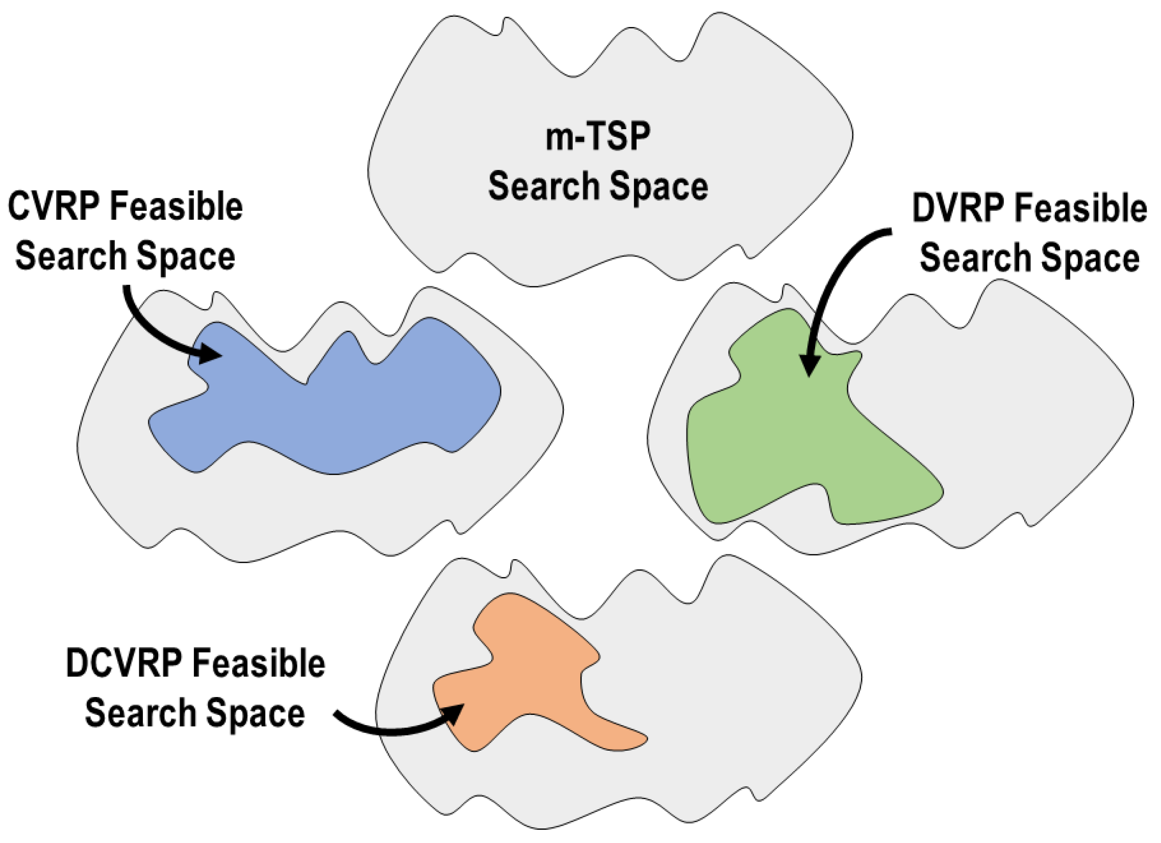
The competitive paradigm [4] has fostered development of many algorithms based only on good empirical performance results. The predominant approach is to argue that a new algorithm is better only because it achieves better results on some standard benchmark instances. The main weakness of this approach, when not accompanied by other methodologies, is that it does not help to understand why an algorithm works well and when it will not be suitable for a specific problem or instance. Fitness Landscape Analysis (FLA) generates an environment to address this deficiency. It aims not to design a new algorithm with better empirical performance, but to explain the behavior of an algorithm based on some properties of the fitness landscape on which it is executed. This is the approach we take in this paper. We aim to explore the impact of vehicle capacity and route duration constraints (see Figure 1) on the overall structure of the search space and on the performance of heuristic algorithms based on local search.

The literature on FLA for VRP is scarce. In particular, to the best of our knowledge, in the context of FLA, our previous research [5] presented the first article to explicitly analyze different levels of constraints in medium-size VRP instances. Other authors have studied the effect of constraints on small instances [6]. The paper analyzed different levels of vehicle capacity in CVRP and ways in which their impact on the search space can be studied with local measures of FLA. In the present paper we expand and complement these results by studying interactions of two VRP attributes (vehicle capacity and route duration constraints), and by using FLA measures of a more global character, as the Local Optima Network Analysis (LONA) measures. In LONA, characteristics of fitness landscapes are studied using a projection in a space formed by the local optima. Thus, the state space is reduced by moving from the solution level (micro scale) with a huge number of solutions to a reduced one (macro/global scale) composed only of local optima.

The paper is structured as follows: Section 2 presents the Mixed Integer Programming (MILP) formulations of the VRP variants studied in this research. Section 3 present some background on Fitness Landscape Analysis (FLA) and leading theories on the structure of fitness landscapes in combinatorial problems, especially from the point of view of Local Optima Network Analysis (LONA). Section 4 describes our experimental design aimed at understanding, with the help of LONA measures, performance of heuristics based on local search when applied to instances of VRP. Section 5 gives the results of Repeated Measures ANOVA applied to determine differences between variants and constraint levels in the measures obtained for LONA. Additionally, we present a bivariate analysis between LONA measures and the heuristic performance; Finally, we present some results related to estimating the difficulty of instances for local search algorithms based on LONA measures and some trends discovered in the data. Section 6 gives a brief discussion of the main contributions of the paper, which include the following:

• To explain the effect of increasing the constraint levels for vehicle capacity and route duration attributes using LONA measures.
• To explore the effect of vehicle capacity and route duration constraints in a Multi-Attribute Vehicle Routing Problem case (DCVRP).
• To predict the difficulty of VRP instances to be solved by local search algorithms using LONA measures.

2. Integer Linear Programing Formulations

Consider the classical Traveling Salesman Problem (TSP) in its multiple-salesmen version (m-TSP) [1], where each customer must be visited exactly once, using one vehicle k of the fleet K of independent vehicles that are available at the central depot. Let V denote the set of points of interest: customers $i\in \{1,2,\cdots ,n\}$ and the central depot 0. The objective is to perform the visits with the minimum total distance travelled, where $c_{i,j}\ge 0$ denotes the distance between the points of interest i and j. In the instances that we study, the distance matrix c is symmetric and corresponds to the Euclidean distances between points on the plane. Binary decision variables $x_{ijk}$ indicate that the point of interest j is visited immediately after i by vehicle k if $x_{ijk}=1$, and otherwise if $x_{ijk}=0$. The following gives one possible formulation of m-TSP.

$$\mathrm{Minimize}\sum _{k\in K}\sum _{i,j\in V}{c}_{i,j}{x}_{i,j,k}$$

(1)

subject to:

$$\begin{array}{cc}\hfill \sum _{i\in V}\sum _{k\in K}{x}_{i,j,k}=1& \forall j\in V\backslash \left\{0\right\}\end{array}$$

(2)

$$\begin{array}{cc}\hfill \sum _{i\in V}{x}_{i,h,k}=\sum _{j\in V}{x}_{h,j,k}& \forall h\in V\backslash \left\{0\right\},k\in K\end{array}$$

(3)

$$\begin{array}{cc}\hfill \sum _{j\in V\backslash \left\{0\right\}}{x}_{0,j,k}=1& \forall k\in K\end{array}$$

(4)

$$\begin{array}{cc}\hfill \sum _{i,j\in S}{x}_{i,j,k}\le \left|S\right|-1& \forall k\in K,S\subseteq V\backslash \left\{0\right\}:\left|S\right|\ge 2\end{array}$$

(5)

$$\begin{array}{cc}\hfill x_{i,j,k}\in \{0,1\}& \forall i,j\in V,k\in K\end{array}$$

(6)

The objective function (1) minimizes the total cost. Expressions (2) ensure that each customer is visited exactly once by a vehicle. Constraints (3) mean that vehicle k leaves customer h if and only if vehicle k arrives at customer h. Constraints (4) indicate that each vehicle leaves the depot exactly once. In (5), sub-tour elimination constraints are applied: Vehicle k does not cycle among the customers in S (with no visit to the central depot). Finally, constraints (6) ensure the nature of the decision variables.

Capacitated Vehicle Routing Problem (CVRP) is one of the most extensively studied extensions of m-TSP, in which each customer has a demand $d_i$ and each vehicle has a limited capacity Q. Thus, CVRP adds to the m-TSP formulation the constraints (7) that ensure that the vehicle capacity is not exceeded on any route [7].

$$\sum _{i\in V\backslash \left\{0\right\}}{q}_i\sum _{j\in V}{x}_{ijk}\le Q,\forall k\in K$$

(7)

Another common variant of VRP, Distance-constrained Vehicle Routing Problem (DVRP), has a constraint on route duration. This constraint implies that vehicles cannot take routes that exceed a total distance L. The formulation presented by Christofides et al. [7] adds the following constraint to the m-TSP:

$$\sum _{i,j\in V}{c}_{ij}{x}_{ijk}\le L,\forall k\in K$$

(8)

If the restrictions on vehicle capacity (7) and route duration (8) are added simultaneously to the m-TSP formulation, the problem is referred to as Distance-constrained and Capacitated Vehicle Routing Problem (DCVRP).

3. Background on Fitness Landscape and Local Optima Network Analysis

For ease of presentation, let us focus in the general descriptions that follow on the case of local search used for maximization problems. Given an instance of a problem, let X be its set of solutions, also called the solution space. Let f be the objective function of the problem, also called its fitness function. Finally, let N be the neighborhood function defined by the local operator used for local search, i.e., a solution y belongs to the neighborhood $N\left(x\right)$ of a solution x if and only if y can be obtained from x by a single application of the local operator. Putting these three together, the triplet $(X,N,f)$ is the fitness landscape of the instance [8]. The notion of a fitness landscape is based on a metaphor commonly used to describe the dynamics of evolutionary algorithms. It considers the solution space together with the neighborhood function to define the search space, over which a landscape surface is defined by the fitness function (height of the solution).

Fitness landscape analysis has been used in different contexts and purposes, from explaining the behavior of algorithms to automated algorithm selection and configuration. Malan et al. [9,10] have conducted two comprehensive reviews of different techniques developed to study fitness landscapes. Contrasting the reviews indicates an evolution of the field from theoretical to more application-focused approaches. Among the types of FLA applications found in the literature, we would like to highlight the following:

• Algorithm performance prediction. Generally, the behavior of a metaheuristic is unpredictable, i.e., we have no formal guarantees on its performance, and it is challenging to predict it when applied to a specific instance. Thus, FLA can be helpful when searching for patterns or general characteristics of problems or instances that can be used as input for performance prediction.
• Understanding complex problems. The approach is based on characterizing problems based on features measured in the underlying fitness landscapes. The central hypothesis motivating this approach is that algorithms or sets of algorithms can have similar behavior on similar problems. Various combinatorial problems, including the VRP family, have been studied under this approach.
• Automated algorithm selection and configuration. Two important tasks are complementary to the analysis of performance of an algorithm: (1) selection of the best algorithm to solve a problem, and (2) selection of the values of the parameters used in a given algorithm. Both propose to search for the best alternative to improve algorithmic performance for solving a given problem. Either approach can benefit from the knowledge that can be extracted from FLA.

Some recent works on Fitness Landscape Analysis can be found in [11,12,13,14].

In this context, the approach of Local Optimal Network Analysis (LONA) is highlighted by Malan [10], as it focuses on the global structure of landscapes and could help understand the behavior of local-search-based algorithms. Malan emphasizes that the broad field of practical application and the evolution of LONA have made it one of the most widely used FLA techniques.

3.1. Local Optima Network Analysis

3.1.1. Representation and Local Operator

For Vehicle Routing Problems, several encodings of solutions are used in search algorithms. The Delimiters representation, one of the most commonly used in the literature, corresponds directly to a set of k individual routes. For a problem with $\left|K\right|$ vehicles, this representation considers an array that contains one substring per trip and $\left|K\right|+1$ copies of the depot used as trip delimiters [15]. For example, the solution $\left[0120340\right]$ represents two routes: In the first, the route starts from the depot, then visits customers one and two, to end at the central depot; In the second, the route starts from the depot to then sequentially visit customers three and four, and conclude at the depot. Note that, as in the three-index-based VRP Mixed Integer Linear Programming (MILP) formulations, the routes/vehicles are distinguishable. Similarly, it is essential to recognize the relationship between the feasible search space, i.e., the search space restricted to feasible solutions, obtained with the Delimiters representation and the set of feasible solutions for the MILP formulations for all variants presented in the paper.

The Delimiters representation supports the application of the original operators developed for TSP and their modifications for VRP. In this context, a specific local operator defines the neighborhood $N\left(x\right)$ associated to a solution x. The function N maps any solution $x\in X$ to the set $N\left(x\right)$ of solutions that can be obtained from x by a single application of the local operator. 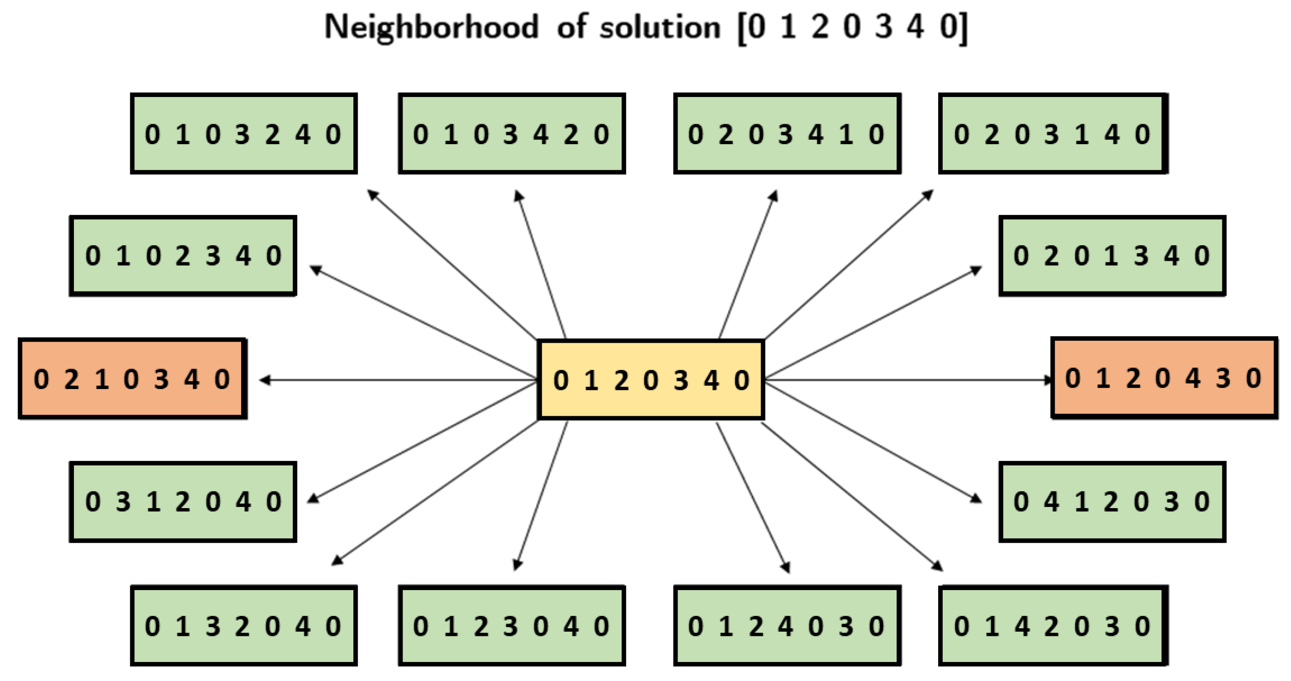If $y\in N\left(x\right)$, then y is a neighbor of the solution x. One of the most common local operators for the VRP is Relocate, which consists of removing a client from its current position and placing it in another. This movement is executed within the same route (intra-route) or between two different routes (inter-route). For more details, Braysy and Gendreau [16] present a review of the main local operators for VRP.

For this article, consider that the solutions of the VRP variants are encoded under the Delimiters representation, and the construction of new solutions is only performed by applying the Relocate operator (Figure 2).

3.1.2. Adjacency of Basins of Attraction

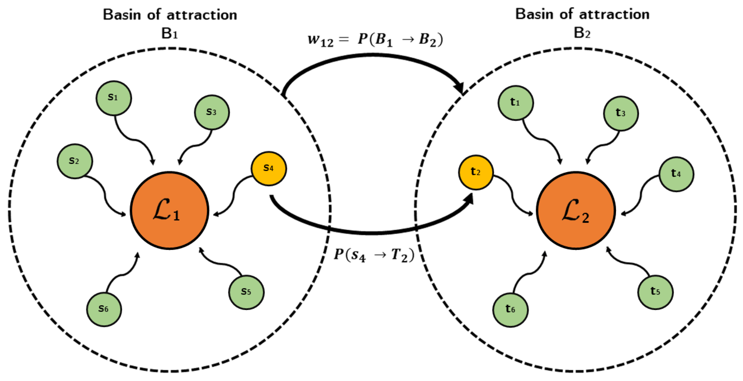
Consider an instance of a maximization problem that has n local optima ${\mathcal{L}}_1,{\mathcal{L}}_2,\cdots ,{\mathcal{L}}_n$. The basin of attraction $b_i$ of each local optimum ${\mathcal{L}}_i$ is defined as $b_i=\{s\in X|h\left(s\right)={\mathcal{L}}_i\}$, where h is an operator that associates a local optimum $h\left(s\right)$ to every solution s. For example, it is common to consider that $h\left(s\right)$ is the fixed point obtained by iteratively applying a hill-climbing algorithm starting from s until reaching convergence. The local optima network of this instance is defined as a weighted graph $G=(V,E)$, where the vertex set V is the set of local optima, and the set of edges E represents the adjacency of the corresponding basins of attraction.

There are two main ways of defining adjacency of basins of attraction described in the literature:

• Basins-transitions requires a complete analysis of the basins of attraction $b_i$ of each local optimum ${\mathcal{L}}_i$. To exemplify, consider two basins of attraction $b_1$ and $b_2$, as shown in Figure 3, corresponding to the local optima ${\mathcal{L}}_1$ and ${\mathcal{L}}_2$, respectively. Likewise, note that the solutions s reach the local optimum ${\mathcal{L}}_1$ by applying the hill-climbing algorithm, just as the solutions t reach ${\mathcal{L}}_2$. Note that both solutions s and t belong to the solution space S, and that the basins of attraction $b_i$ generate a partition over S such that: $S={\bigcup }_{i\in LO}{b}_i$ and $\forall i\in S,$$\forall i\ne j,b_i\cap b_j=Ø$.

The arc $e_{1,2}$ from the local optimum ${\mathcal{L}}_1$ to ${\mathcal{L}}_2$ exists if and only if there exist $s\in b_1$ and $t\in b_2$ such that $t\in N\left(s\right)$. In this case, the transition probability of passing from a solution $s_i\in b_1$ to a solution $t_k\in b_2$ is ${\displaystyle P(s_i\to t_k)=\frac{1}{\left|N\right(s_i\left)\right|}}$ if $t_k\in N\left(s_i\right)$, and otherwise $P(s_i\to t_k)=0$. Moreover, the probability $P(s_i\to b_2)$ of transition from a solution $s_i$ to the basin of attraction $b_2$ is computed by summing up the individual transition probabilities of $s_i$ with each solution belonging to $b_2$. Finally, the weight $w_{1,2}$ of the arc $e_{1,2}$ is the average transition probability to $b_2$ of the solutions in $b_1$.

2.

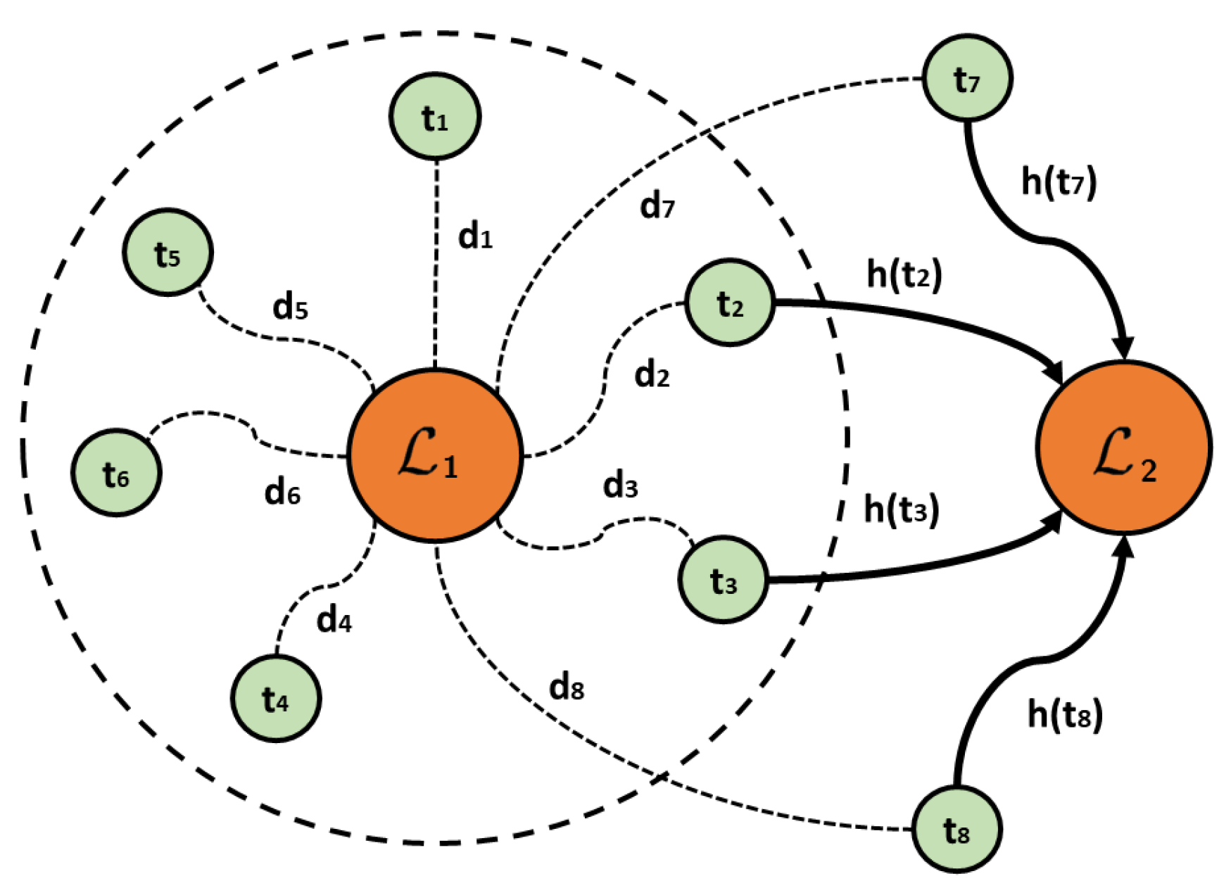
Escape-edges is based on the distance between each pair of local optima. This new way of establishing the adjacency relationship between local optima was proposed to solve the problem of producing very dense networks that required exhaustive sampling of the basins of attraction. The weights $w_{ij}$ based on Escape-edges do not require a complete calculation of the basins of attraction [17]. The weights are defined according to a distance function d (minimum number of moves between two solutions) and a positive integer $D>0$. The edge $e_{ij}$ between ${\mathcal{L}}_i$ and ${\mathcal{L}}_j$ exists only if there exists a solution t such that $d(t,{\mathcal{L}}_i)\le D$ and $h\left(t\right)={\mathcal{L}}_j$. The weights $w_{ij}$ are established by counting the number of solutions that are in the basin of attraction of ${\mathcal{L}}_j$ and at a distance less than or equal to D from ${\mathcal{L}}_i$. The number of solutions that satisfy this condition is normalized by the total number of solutions at a distance less than or equal to D from ${\mathcal{L}}_i$ (regardless of whether they belong to the basin of attraction of ${\mathcal{L}}_j$). Figure 4 presents a schematic of the relationship between local optima using transitions based on Escape-edges.

Local Optima Network Analysis (LONA) is a topic in the literature on Fitness Landscape Analysis (FLA) of combinatorial problems that has started to be studied only recently. The problem that has been studied with LONA techniques the most is the NK model. It was used by Ochoa et al. [18] to introduce LONA, and has been studied later for further advances in the development of this tool. In the case of the Quadratic Assignment Problem, Chicano et al. [19] used LONA to predict the performance of search algorithms. With the same motivation of performance prediction, Pavelski et al. [20] used LONA to study two Iterated Greedy algorithms for the Flow Shop Scheduling problem. Chicano et al. [21] proposed the same for the MAX-3SAT problem. In the context of VRP, Ochoa et al. [22] performed a mapping of the global structure for TSP, showing that the difficulty of the search is related to the presence of multiple funnels in the landscape. Additionally, they reported high levels of neutrality. For VRP variants and practical uses of LONA, Lipinski et al. [23] present an evolutionary algorithm for solving the Inventory Routing Problem (IRP), which includes an improvement mechanism based on Simulated Annealing that consists of calculating the transition probabilities obtained with LONA and using them to guide the search.

4. Methods

This section presents the main aspects of the experimental design we use for studying different VRP variants under multiple constraint levels: (a) construction of instances for each problem, (b) creation of local optima networks, (c) computation of LONA measures, (d) computation of measures related to the difficulty in local search, and (e) analysis of relationships between the LONA measures and the difficulty of local search.

4.1. Instance Creation

To analyze the role of constraints, we create new experimental instances based on 61 base instances taken from the literature. They are selected among the base instances used in our previous study [5] by the criterion of having at most 60 nodes. For each base instance, we create a feasibility sample of ${10}^5$ m-TSP solutions where each Delimiter representation is chosen uniformly at random, with the depot 0 repeated $k-1$ times, where k is the number of vehicles. The sample thus obtained is used to compute four constraint levels for each restriction (vehicle capacity and route duration) as described in the following:

• For CVRP, for each base instance, we create an experimental instance at 4 levels: Level 0 where all m-TSP solutions are feasible; Level 1 in which 75% of m-TSP solutions are feasible; Level 2 such that 50% of m-TSP solutions are feasible; and Level 3 where 25% of m-TSP solutions are feasible. For each base instance, we choose the minimum capacity for which the required proportion of the respective feasibility sample is feasible for CVRP.
• For DVRP, we proceed like for CVRP, only considering restrictions on route durations instead of vehicle capacities. We also create experimental instances at 4 levels: Level 0 where all solutions are feasible for DVRP, Level 1 in which 50% of the solutions are feasible), Level 2 such that 30% of the solutions are feasible, and Level 3 where 10% of the solutions are feasible.
• For the DCVRP case, we create only one experimental instance for each base instance. We set both the vehicle capacity and the route duration at the value that comes from the corresponding Level 3. Note that, unlike the cases of CVRP and DVRP in which the proportion of feasible solutions is pre-set, in DCVRP experimental instances this proportion changes from one to another.

From the formal point of view, an m-TSP instance considers only the locations of the customers (or the distances between them) and the number of vehicles. For CVRP, the customer demands and the vehicle capacity are incorporated. In DVRP, we add the maximum route length. Finally, for DCVRP, the features of DVRP and CVRP are incorporated together. However, Level 0 experimental instances for CVRP and DVRP based on a fixed base instance have the same feasible solutions with the same value of the objective function, in spite of formally corresponding to different instances (of different problems). Thus, they yield the same fitness landscape. Adopting the point of view of fitness landscapes, such two experimental instances are considered the same for our analysis. So, based on 61 base instances, we create the following: 61 experimental instances for Level 0, 366 experimental instances for Levels 1, 2, and 3 of CVRP and DVRP, and 61 experimental instances for DCVRP. In total, we get 488 experimental instances.

We create several datasets to achieve the research objectives: The main is the MAVRP dataset [24] containing all the measurements taken on the local optima network and the local search behavior for each one of the 488 experimental instances. The CVRP dataset is obtained from the MAVRP dataset by considering only the 244 experimental instances relevant for analyzing CVRP: Levels 0 through 3 for CVRP. In an analogous way, the DVRP dataset considers the 244 experimental instances relevant for DVRP. Finally, the DCVRP dataset is based on 183 experimental instances: Level 3 for CVRP and DVRP, and the DCVRP experimental instances.

4.2. Local Optima Network Construction

4.2.1. Nodes: Local Optima

For each experimental instance, we consider a random feasible solution sample $\mathcal{SP}$ of ${10}^3$ solutions where each Delimiter representation is chosen uniformly at random, with the depot 0 repeated $k-1$ times, where k is the number of vehicles. However, we keep the solution only if it is feasible for the experimental instance. Each element of the feasible solution sample is used as the initial solution for the First-Improvement hill-climbing algorithm (Algorithm 1) to obtain the corresponding local optimum. We use $LO\left(\mathcal{SP}\right)$ to denote the local optima sample, the set of local optima thus obtained.

Algorithm 1 First-Improvement Hill-Climbing

procedure First-Improvement Hill-Climbing     $x\leftarrow$ initial solution     while x is not a Local Optimum do         $x^{\prime }\leftarrow$ random solution from $\mathcal{N}\left(x\right)$         if $f\left(x^{\prime }\right)<f\left(x\right)$ then            $x\leftarrow x^{\prime }$         end if     end while   end procedure

4.2.2. Edges: Relocate Distance

Most local operators that have been defined in the literature on local-search-based algorithms for VRP are inspired by those used for TSP [16]. The majority of them are symmetric, i.e., if a solution y can be obtained by one application of the local operator to a solution x, then the same holds in the opposite direction. And it is the case for the Relocate operator considered in this research.

Each local operator is associated to a notion of distance. Given two solutions x and y, the corresponding distance $d(x,y)$ is the minimum number of applications of the local operator necessary to transform x into y. In other words, computing $d(x,y)$ corresponds to computing a shortest path from x to y in the corresponding search space.

For many local operators, the corresponding distances in the TSP search space can be computed efficiently (e.g., such is the case for the Relocate and Exchange operators), which results in their wider use. But in some cases computing the corresponding distance is NP-hard (e.g., it holds for the distance based on 2-Opt). The reader is referred to the survey by Schiavinotto and Stützle [25] for more details (therein, Relocate, Exchange and 2-Opt are called insert, interchange and 2-edge-exchange, respectively). These complexity results can be easily adapted to the versions of these operators for m-TSP, thus computing the distance in a m-TSP space is polynomial for Relocate and Exchange, whereas it is NP-hard for 2-Opt.

Constraining the search space tends to make computing the distance harder. For example, computing a shortest path between two solutions of TSP in the search space generated by 2-Opt is “only” NP-complete when any solution can be visited along the way. Adding a restriction that only TSP routes of duration at most a certain constant K can be visited along the way makes the problem of computing a shortest path PSPACE-hard. This can be seen with a simple reduction from the Hamiltonian Cycle Reconfiguration problem based on 2-Opt, that was proved by Takaoka [26] to be PSPACE-complete. Thus computing the 2-Opt distance in DVRP is PSPACE-hard.

Up to out knowledge, no results on the complexity of reconfiguration for Hamiltonian Cycle (or other VRP variants) with other local operators have been published. Nevertheless, we believe that computing the distances based on Relocate or Exchange in the solution space of DVRP, CVRP or DCVRP is at least NP-hard. This intuition comes from the fact that even reconfiguration problems based on very simple optimization problems tend to be hard. For example, the Shortest Path problem in general unweighted graphs can be solved in linear time (for example, using Breadth-First Search), but the Shortest Path Reachability problem (its reconfiguration version) is PSPACE-complete event when limited to unweighted graphs of bounded bandwidth [27]. For this reason, we limit ourselves to computing the distances between solution in the underlying m-TSP space even when working with DVRP, CVRP or DCVRP.

In this research, we analyze search spaces based on the Delimiters representation and the Relocate operator. Sörensen and Schittekat [15] described in depth the use of the Relocate Distance based on the Delimiters representation for VRP. Consequently, for each experimental instance, we built the corresponding local optima network as follows:

• We take the corresponding local optima sample $LO\left(\mathcal{SP}\right)$ and construct a complete graph using every local optimum ${\mathcal{L}}_i$ as vertex $v_i$ and every pair of local optima $(\mathcal{L}i,{\mathcal{L}}_j)$ as edge $e_{ij}$. Then, we calculate the Relocate Distance $d({\mathcal{L}}_i,{\mathcal{L}}_j)$ for every pair of local optima.
• We delete every edge $e_{ij}$ for which $d({\mathcal{L}}_i,{\mathcal{L}}_j)>D$. The parameter D is set to the percentile 25 (first quartile) of all the distances computed in the step 1.

Note that the local optima network is undirected, because the distances between the local optima are symmetric.

4.3. Local Optima Network Analysis: Measures

4.3.1. Measure 1: Density

The Density measure presented in Equation (9) is defined as the ratio of observed edges to the number of possible edges for a given network. Let $\tau$ denote the order of a network, which refers to the number local optima. The number of all possible edges for an undirected network of order $\tau$ is $\tau (\tau -1)/2$. Let $\epsilon$ be the number of edges in the network. Then, Density $DS$ can be expressed as:

$${\displaystyle DS=\frac{2\epsilon }{\tau (\tau -1)}}$$

(9)

4.3.2. Measure 2: Transitivity

Transitivity, also known as Clustering Coefficient is a measure of the tendency of the nodes to cluster together. Perfect transitivity implies that, if local optimum ${\mathcal{L}}_1$ is connected (through an edge) to local optimum ${\mathcal{L}}_2$, and ${\mathcal{L}}_2$ is connected to local optimum ${\mathcal{L}}_3$, then ${\mathcal{L}}_1$ is connected to ${\mathcal{L}}_3$ as well. The Clustering coefficient T of a network is the average clustering coefficient $T_i$ for all local optima ${\mathcal{L}}_i$ in the network; Thus, the computation of T is as follows:

$$T=\frac{{\displaystyle \sum _{i=1}^{\tau }{T}_i}}{\tau }\mathrm{with}{T}_i=\frac{2Tr\left({\mathcal{L}}_i\right)}{deg\left({\mathcal{L}}_i\right)(deg\left({\mathcal{L}}_i\right)-1)},\forall i\in \{1,2,..,\tau \}$$

(10)

$Tr\left({\mathcal{L}}_i\right)$ is the number of triangles through local optimum ${\mathcal{L}}_i$ and $deg\left({\mathcal{L}}_i\right)$ is the degree of $\mathcal{L}$. $T=1$ implies perfect transitivity, i.e., a network whose connected components are all cliques. $T=0$ implies no triangles (transitive relations) in the network.

4.3.3. Measure 3: Assortativity

Assortativity measures the tendency of similar local optima to be grouped. In this work, we measure Assortativity based on node degree $deg\left({\mathcal{L}}_i\right)$ of each local optimum ${\mathcal{L}}_i$. Let $P=\{p_0,p_1,..,p_k\}$ be the degrees of the corresponding local optima in the network. Then, we define the following parameters:

• Mixing matrix$M_{p_u,p_v}$ represents the number of edges from nodes with degree $p_u$ to nodes with degree $p_v$.
• Degree correlation matrix$c_{p_u,p_v}$ represents the probability of finding nodes with degrees $p_u$ and $p_v$ as the two ends of an edge selected at random. Thus, ${\displaystyle c_{p_u,p_v}=\frac{M_{p_u,p_v}}{\epsilon }}$.
• Degree probability$q_{p_u}$ is the probability that there is a node with degree $p_u$ at the end of the randomly selected edge. Thus, ${\displaystyle q_{p_u}=\sum _{p_v}^P{c}_{p_u,p_v}}$.

The Assortativity can be described using the Degree Correlation Coefficient A proposed by Newmann (citar), that is defined as:

$$A=\sum _{p_u\in P}\sum _{p_v\in P}\frac{p_u{p}_v(c_{p_u,p_v}-q_{p_u}{q}_{p_v})}{{\sigma }^2}\mathrm{with}{\sigma }^2=\sum _{p_v\in P}{p}_v^2{q}_{p_v}-{\left(\sum _{p_v\in P}{p}_v{q}_{p_v}\right)}^2$$

(11)

Hence, A is the Pearson correlation coefficient between the degrees found at the two end of the same edge. For $A>0$ the network is assortative, for $A=0$ the network is neutral and for $r<0$ the network is disassortative.

4.3.4. Measure 4: Distance Ratio

The Distance Ratio estimates the closeness between local optima. For this, we calculate the median distance ($med\left(d\right)$) between the local optima and normalize using the diameter of the search space (equal to the number of customers $\left|V\right|-1$). Thus, networks constructed from different instances of the VRP are comparable. Therefore, the Distance Ratio (DR) computation is as follows:

$$DR=\frac{med\left(d\right)}{\left|V\right|-1}$$

(12)

Consequently, the closer DR is to zero, the closer the local optima of the network tend to be to each other.

4.3.5. Measure 5: Quality of Local Optima Sample

The Hill-Climbing Gap (HC-Gap) measure explores the quality of the local optima sample. We use the Lin–Keninghan–Helgsaun (LKH) algorithm and extensions [28] to estimate the global optimum for each experimental instance (the best of ten runs). The solution obtained with LKH on m-TSP, CVRP, and DCVRP instances offers a sufficiently good (potentially optimal) benchmark to measure the quality of other solutions. The benchmark results presented in the cited reports indicate that the LKH algorithm achieved the best-known or new best solutions for 96.85%, 72.88%, and 81.81% of m-TSP, CVRP and DCVRP instances tested, respectively. Moreover, the experiments presented by Helgsaun cover computationally more challenging instances than those used in this research. The computation of the Gap measure (%) relates the median fitness value of the local optima sample computed with First-Improvement Hill-Climbing ($med\left(f_{\mathcal{L}}\right)$) and the best fitness value of LKH solutions ($f_{LKH}$) using the following definition:

$$HC-Gap=100\times \frac{med\left(f_{\mathcal{L}}\right)-f_{LKH}}{f_{LKH}}$$

(13)

Thus, better quality solutions have a HC-Gap(%) close to zero.

4.3.6. Measure 6: Number of Steps to Local Optimum

The Number of steps to local optimum $S{T}_i$, executed when applying First-Improvement Hill-Climbing, estimates the closeness between local optima ${\mathcal{L}}_i$ and their respective starting points $S{P}_i({\mathcal{L}}_i=HC\left(S{P}_i\right))$. To compute the Steps measure for an experimental instance, we use the median $med\left(ST\right)$, over the feasible solution sample $\left(SP\right)$, of the number of steps performed by the local-search-based algorithm to reach the respective local optimum. Similarly to the Distance Ratio measure, the number of steps is adjusted considering the diameter of the search space in the respective instance. So we get the following formula:

$$Steps=\frac{med\left(ST\right)}{\left|V\right|-1}$$

(14)

Consequently, the closer Steps is to zero, the closer the local optima of the network tend to be to their respective starting points.

4.3.7. Measure 7: Dispersion

The Dispersion measures the variability of fitness values of the local optima in the network. We use the Dispersion Coefficient $DC$ based on the coefficient of variation. The DC is the ratio between the standard deviation $stddev\left(f_{\mathcal{L}}\right)$ and the mean $\overline{f_{\mathcal{L}}}$ of the fitness in the local optima sample. The coefficient of variation is applicable in our research because it is dimensionless (i.e., independent of the measurement unit) and is, therefore, comparable between experimental instances.

$$DC=\frac{stddev\left(f_{\mathcal{L}}\right)}{\overline{f_{\mathcal{L}}}}$$

(15)

Hence, when $DC$ is close to zero, the local optima tend to have similar fitness values.

4.4. Performance Measure: Difficulty for Local Search

The Simulated-Annealing Gap (SA-Gap) measure explores the performance of local search algorithms. As we did for computing the HC-Gap, we use the Lin–Keninghan–Helgsaun (LKH) algorithm and extensions to compute the SA-Gap measure (%). The measure relates the median fitness value of twenty runs computed with Simulated Annealing ($med\left(f_{\mathcal{SA}}\right)$) and the best fitness value of LKH solutions ($f_{LKH}$) using the following definition:

$$Gap=100\times \frac{med\left(f_{\mathcal{SA}}\right)-f_{LKH}}{f_{LKH}}$$

(16)

Thus, a SA-Gap(%) close to zero implies a better algorithmic performance.

We generate an initial solution for SA from a permutation of the customers chosen uniformly at random (TSP solution space), by applying a Split algorithm [5,29]. Then, with each move, a neighboring feasible solution is chosen—as is usual in SA algorithms for VRP. We propose an SA parametrization that uses an initial temperature $T=1000$, and the temperature varies across the iterations using a linear cooling schedule with a fixed cooling rate t = 0.9 [30]. For each temperature, the algorithm performs ${\left|V\right|}^2$ iterations.

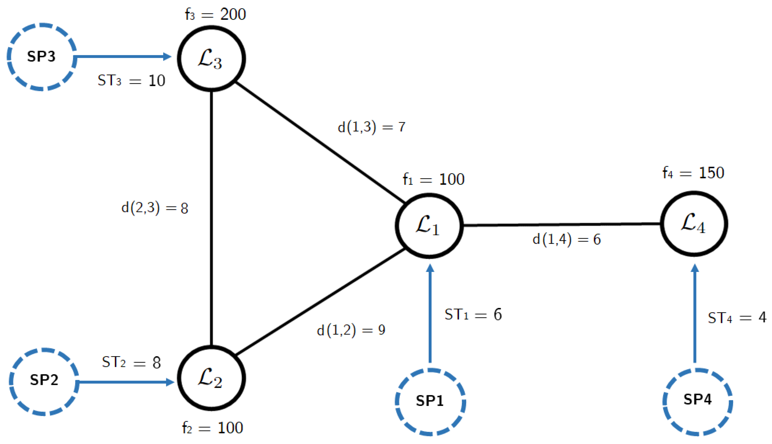
4.5. An Example of LONA and Performance Measures

Consider the local optima network presented in Figure 5, which is based on a local optima sample of $({\mathcal{L}}_1$, ${\mathcal{L}}_2$, ${\mathcal{L}}_3$, ${\mathcal{L}}_4)$ obtained from a feasible solution sample of $(S{P}_1$, $S{P}_2$, $S{P}_3$, $S{P}_4)$. The local optima network has edges: $\left(\right({\mathcal{L}}_1$, ${\mathcal{L}}_2)$, $({\mathcal{L}}_1,$${\mathcal{L}}_3)$, $({\mathcal{L}}_1,$${\mathcal{L}}_4),$$({\mathcal{L}}_2,$${\mathcal{L}}_3\left)\right)$. It is obtained for a VRP instance with ten customers.

The fitness levels of the local optima are $f_{\mathcal{L}}=(50,100,200,150)$, representing the node weights; and the respective edges have weights $d=(9,7,6,8)$ determined by the relocate distance between the corresponding local optima, as shown in Figure 5. Moreover, the median fitness value of twenty runs computed with Simulated Annealing is $f_{\mathcal{SA}}=95$. Thus, the LONA and Performance measures would be calculated as follows:

• Density (DS): The number of arcs that could exist in the network is six, equivalent to ${\displaystyle \frac{\tau (\tau -1)}{2}}$. In the network shown in Figure 5, only four of the six possible arcs exist, so the network density is $DS=4/6=0.667$.
• Transitivity (T): The transitivity coefficient corresponds to the fraction of triads that are closed. In the above example, for instance, there are five triads: one centered at ${\mathcal{L}}_2$, one at ${\mathcal{L}}_3$, and three at ${\mathcal{L}}_1$. Three of them are closed triads (centred in ${\mathcal{L}}_1$, ${\mathcal{L}}_2$ and ${\mathcal{L}}_3$, respectively), and two are open (both centred in ${\mathcal{L}}_1$). Hence the transitivity coefficient is $T=3/5=0.6$
• Assortativity (A): To calculate the assortative coefficient, it is necessary to calculate the degree of each node and relate it to adjacent ones (see

  Table 1. Degree of each pair of adjacent nodes in the example.

  ${\mathcal{L}}_{\mathit{i}}$	${\mathcal{L}}_1$	${\mathcal{L}}_1$	${\mathcal{L}}_1$	${\mathcal{L}}_2$	${\mathcal{L}}_2$	${\mathcal{L}}_3$	${\mathcal{L}}_3$	${\mathcal{L}}_4$
  ${\mathcal{L}}_j$	${\mathcal{L}}_2$	${\mathcal{L}}_3$	${\mathcal{L}}_4$	${\mathcal{L}}_1$	${\mathcal{L}}_3$	${\mathcal{L}}_1$	${\mathcal{L}}_2$	${\mathcal{L}}_1$
  $deg\left({\mathcal{L}}_i\right)$	3	3	3	2	2	2	2	1
  $deg\left({\mathcal{L}}_j\right)$	2	2	1	3	2	3	2	3

  ). In this case, the relationship between the degrees of neighboring nodes is inversely proportional, indicating a disassortative network ($A=-0.714$).
• Distance Ratio (DR): The distances between local optima that are presented in the example are $d({\mathcal{L}}_1,{\mathcal{L}}_2)=9$, $d({\mathcal{L}}_1,{\mathcal{L}}_3)=7$, $d({\mathcal{L}}_1,{\mathcal{L}}_4)=6$ and $d({\mathcal{L}}_2,{\mathcal{L}}_3)=8$. In that context, the median of the distances is 7.5. Furthermore, the representation of the solutions for the VRP instance for which the local optima network was constructed has a search space diameter of ten ($\left|V\right|-1$), considering that the instance has ten customers. Thus, the distance ratio $DR=7.5/10=0.75$.

The local search measures for the examples are:

• Quality of Local Optima Sample (HC-Gap): The fitness of the local optima are $f_{LO}=(100,100,200,150)$. Therefore, the median $med\left(f_{LO}\right)=125$. If the best solution of the LKH algorithm is $f_{LKH}=90$, then the $Gap=38.8\%$.
• Steps to Local Optima (Steps): The number of steps from the starting points (SP) to the local optima (LO) are $S{T}_1=6$, $S{T}_2=8$, $S{T}_3=10$ and $S{T}_4=4$. So the median $median\left(ST\right)=7$. Similar to the distance ratio, it is adjusted using the search space diameter. For this network the measure $Steps=0.7$.
• Dispersion Coefficient (DC): The local optima network has a standard deviation of the fitness of 40.82 and a mean of 150. Therefore, the dispersion coefficient $DC=0.272$.
• Performance Measure (SA-Gap): The median fitness value of Simulated Annealing is $f_{\mathcal{SA}}=95$ and the best solution of the LKH algorithm is $f_{LKH}=90$, then the $SA-Gap=5.55\%$.

4.6. Guidelines to Analyze Local Search Performance Based on Local Optima Network Analysis

Here we present our guidelines for analyzing the performance of local search (exemplified by SA) in VRP using LONA. For this research, the main objectives are:

• To determine whether measures based on information obtained from LONA can be useful to detect differences between VRP instances. The differences are studied using the CVRP, DVRP and DCVRP datasets.
• To understand the relationship that exists between pairs of LONA measures. We seek to describe changes in the direction and strength of associations between variables when exploring search spaces at different levels of constraint, both for individual attributes (CVRP and DVRP) and the multi-attribute case (DCVRP).
• To explore whether LONA measures are related with the behavior observed in local search algorithms.

The main steps of the research methodology are as follows:

• Preliminary analysis of local optima networks: To determine the differences between the VRP instances under study, we perform an analysis based on Repeated Measures ANOVA to detect significant differences in the LONA measures. This procedure is performed between variants (Multi-Attribute Perspective) and between constraint levels (Single-Attribute Perspective).
  • Single-Attribute Perspective: We use the CVRP and DVRP datasets independently, emphasizing differences in LONA measures between constraint levels.
  • Multi-Attribute Perspective: We use the DCVRP dataset, emphasizing the differences in LONA measures between the individual attributes of distance or capacity (Level 3) with those obtained when both are studied together.
• Correlation analysis: We use the Spearman Rank Correlation coefficient [31] to analyze the strong monotonic correlations between the LONA measures and whether these correlations hold between variants and constraint levels. Thus, we have a first approach to evaluate the effect that the restrictions have on the relationships between the measures we use. Therefore, this is an exploratory step in the study of the behavior of the LONA measures. We study the correlations in the CVRP and DCVRP datasets at each constraint level. In addition, we present the Spearman Rank Correlations obtained using the DCVRP dataset.
• Prediction of Difficulty for Local Search: Finally, we use the method of Logistic Regression to predict the difficulty of the instances using LONA measures. For this task, we propose a discretization of the performance measures in the CVRP, DVRP and DCVRP datasets. We split the instances in each one of these datasets into two equal-sized classes, based on the local search measures: Low (≤$median$) and High (>$median$). These categories let us capture the performance behavior and explore the underlying patterns associated with the LONA measures. We apply Logistic Regression over each dataset and extract the performance evaluation metrics using a re-sampling technique. For each one among the CVRP, DVRP and DCVRP datasets, we create 100 sample datasets that contain only one constraint level for each base instance. In this way, we create a Logistic Regression model for each sample dataset, and based on all the sample datasets, we obtain confidence intervals for the performance evaluation of the Logistic Regression used a method for classification [5].

5. Results

5.1. Preliminary Analysis of Local Optima Networks

The first objective is to understand the differences among the VRP variants considered in the research. In this context,

Table 2. Results for Repeated Measures ANOVA for LONA measures-Single-Attribute Perspective.

Measures	DVRP	CVRP
Density	×	×
Transitivity	×	×
Assortativity	×	✓
Distance Ratio	✓	×
Dispersion Coefficient	×	✓
Quality of Local Optima	✓	✓
Steps to Local Optima	✓	✓

and

Table 3. Results for Repeated Measures ANOVA for LONA measures—Multi-Attribute Perspective.

	DVRP	DVRP	CVRP
Measures	CVRP	DCVRP	DCVRP
Density	×	×	×
Transitivity	×	×	×
Assortativity	✓	✓	×
Distance Ratio	✓	✓	✓
Dispersion coefficient	✓	✓	✓
Quality of local optima	✓	✓	✓
Steps to Local Optima	✓	✓	✓

present the analysis based on Repeated Measures ANOVA on the single attribute datasets (CVRP and DVRP) and the multi-attribute dataset (DCVRP), respectively.

5.1.1. Single-Attribute Perspective

The analyses work with the following null ($H_0$) and alternative ($H_1$) hypotheses:

• $H_0$: The corresponding LONA measure at different constraint levels has the same population mean. Thus, for the CVRP and DVRP datasets, $H_0:{\mu }_{\mathrm{Level}0}$$={\mu }_{\mathrm{Level}1}$$={\mu }_{\mathrm{Level}2}$$={\mu }_{\mathrm{Level}3}$ for each measure.
• $H_1:$ At least one population mean is different from the rest.

We do these analyses to know if different constraint levels lead to significantly different values of LONA measures. If the Fisher-test is significant (✓), it implies that at least two groups among those compared are significantly different ($\alpha \le 0.05$); otherwise (×) there is no evidence of a significant difference between the groups. The results are shown in Table 2.

For the distance attribute (DVRP dataset), most LONA measures present no significant differences. However, there are differences in the Distance Ratio. The result indicates that when considering a more constrained landscape, the local optima tend to present a greater distance between them. On the other hand, the measures related to local search show significant differences in Quality of Local Optima and Steps to Local Optima. Note that the local search is performed on constrained landscapes, so the visited solutions must be feasible. We observe that, in a more constrained landscape, the local optimum reached by Hill-Climbing is closer to the starting point and the median quality of local optima is better. On the other hand, no significant difference is observed in the fitness dispersion; Dispersion Coefficient does not change between the different constraint levels.

On the other hand, the capacity attribute (CVRP dataset) has different results from those obtained for the distance attribute. For the LONA measures, Density and Transitivity of the network maintain the behavior observed for the distance attribute. However, we find significant differences concerning Assortativity. At this point, it is important to note that the networks present low Assortativity (mean $A=0.07$ at level 0 and $0.12$ at level 3 of the CVRP). That is, local optima with a similar degree tend to be more connected. Similarly, for the local search measures, the results for Quality of Local Optima and Steps to Local Optima are maintained. However, for the capacity attribute, there are significant differences in Dispersion Coefficient. Thus, the dispersion is slightly higher at higher constraint levels.

It is common for the datasets that we study that we observe no differences for Density and Transitivity, even when both types of constraints are involved. This indicates no significant differences in the number of edges or the tendency to cluster in the network. On the other hand, there are some differences in the distribution of local optima, both in Distance Ratio and Assortativity.

5.1.2. Multi-Attribute Perspective

The analyses work with the following null ($H_0$) and alternative ($H_1$) hypotheses:

• $H_0$: ${\mu }_{\mathrm{CVRP}\mathrm{Level}3}={\mu }_{\mathrm{DVRP}\mathrm{Level}3}$ and $H_1$: The population mean is different.
• $H_0$: ${\mu }_{\mathrm{DVRP}\mathrm{Level}3}$$={\mu }_{\mathrm{DCVRP}}$ and $H_1$: The population mean is different.
• $H_0$: ${\mu }_{\mathrm{CVRP}\mathrm{Level}3}={\mu }_{\mathrm{DCVRP}}$ and $H_1$: The population mean is different.

For the Multi-Attribute Perspective, we observe that for DVRP and CVRP, there are significant differences in the behavior observed for the LONA measures in DCVRP. The results imply a difference in the overall structure of the search space when distance and capacity attributes are considered simultaneously. The above is valid for all measures, except for network density and transitivity, in both CVRP and DVRP. Furthermore, in the case of CVRP, there are also no significant differences from DCVRP in network assortativity.

5.2. Correlation Analysis of LONA Measures

The previous subsection presents the univariate analysis of LONA. In contrast, here we seek to expand the research to a bivariate view. From this perspective, the use of Spearman Rank Correlation is proposed to quantify the relationship between pairs of measures without assuming linear behavior.

Table 4. Spearman Rank Correlation for LONA measures, comparison for the capacity attribute. Bold values denotes the coefficients that are significant at a $\alpha =0.05$.

Measure 1	Measure 2	MTSP	CVRP75	CVRP50	CVRP25	DCVRP
Quality of	Dispersion Coefficient	0.83	0.55	0.61	0.58	0.59
Local	Steps to Local Optima	0.24	0.28	0.34	0.42	0.43
Optima	Density	0.05	0.13	−0.12	−0.10	−0.18
Sample	Transitivity	−0.18	0.004	0.08	−0.09	−0.13
	Assortativity	−0.31	−0.24	−0.28	−0.46	−0.47
	Distance Ratio	0.46	0.73	0.67	0.71	0.77
Dispersion	Steps to Local Optima	−0.04	−0.10	0.07	0.10	0.16
Coefficient	Density	0.08	−0.08	−0.12	−0.21	−0.22
	Transitivity	0.06	0.20	0.28	0.34	0.35
	Assortativity	−0.09	−0.17	−0.18	−0.16	−0.23
	Distance Ratio	0.16	0.30	0.27	0.29	0.32
Steps to	Density	−0.31	0.03	−0.13	−0.10	−0.17
Local Optima	Transitivity	−0.16	0.10	0.23	0.08	0.11
	Assortativity	−0.38	−0.51	−0.67	−0.81	−0.81
	Distance Ratio	0.49	0.45	0.54	0.51	0.57
Density	Transitivity	0.31	0.27	0.43	0.37	0.41
	Assortativity	−0.24	0.10	0.02	0.05	0.08
	Distance Ratio	−0.05	0.14	−0.01	−0.09	−0.21
Transitivity	Assortativity	0.23	0.05	−0.19	−0.10	−0.08
	Distance Ratio	−0.64	−0.09	−0.02	0.25	−0.27
Assortativity	Distance Ratio	−0.56	−0.29	−0.40	−0.57	−0.59

and

Table 5. Spearman Rank Correlation for LONA measures, comparison for the distance attribute. Bold values denotes the coefficients that are significant at a $\alpha =0.05$.

Measure 1	Measure 2	MTSP	DVRP50	DVRP30	DVRP10	DCVRP
Quality of	Dispersion Coefficient	0.83	0.83	0.82	0.81	0.59
Local	Steps to local optima	0.24	0.23	0.26	0.28	0.43
Optima	Density	0.05	−0.18	−0.31	0.05	−0.18
Sample	Transitivity	−0.18	−0.30	−0.33	−0.08	−0.13
	Assortativity	−0.31	−0.15	−0.10	−0.24	−0.47
	Distance Ratio	0.46	0.46	0.47	0.50	0.77
Dispersion	Steps to local optima	−0.04	−0.06	−0.05	−0.03	0.16
Coefficient	Density	0.08	−0.18	−0.24	0.04	−0.22
	Transitivity	0.06	−0.13	−0.17	−0.02	0.35
	Assortativity	−0.09	0.07	0.10	−0.01	−0.23
	Distance Ratio	0.16	0.17	0.18	0.17	0.32
Steps to	Density	−0.31	−0.25	−0.34	−0.15	−0.17
local optima	Transitivity	−0.16	−0.20	−0.21	−0.02	0.11
	Assortativity	−0.38	−0.43	−0.41	−0.48	−0.81
	Distance Ratio	0.49	0.48	0.49	0.49	0.57
Density	Transitivity	0.31	0.33	0.38	0.33	0.41
	Assortativity	−0.24	−0.17	−0.12	−0.18	0.08
	Distance Ratio	−0.05	−0.09	−0.20	0.01	−0.21
Transitivity	Assortativity	0.23	0.44	0.43	0.32	−0.08
	Distance Ratio	−0.64	−0.72	−0.70	−0.50	−0.27
Assortativity	Distance Ratio	−0.56	−0.57	−0.45	−0.57	−0.59

show that Quality of Local Optima Sample has a moderately high and monotonically positive relationship with the Distance Ratio. Thus, the HC-Gap tends to be larger when the local optima are more distant. Moreover, we observe that this relationship is stronger at higher constraint levels.

Another aspect to mention is that Quality of Local Optima Sample has a moderately low and monotonically negative relationship with Assortativity. As with Distance Ratio, this behavior is stronger at higher levels of constraint for the capacity attribute. Local optima networks with more connections between local optima with a similar degree tend to produce a smaller HC-Gap.

Additionally, we observe that Dispersion Coefficient has a moderately high and monotonically positive relationship with Quality of Local Optima Sample. Thus, we observe a large HC-Gap when the variability in the fitness of the local optima is higher. The relationship between DC and HC-Gap is stronger in instances with lower constraint levels. Furthermore, the relationship is stronger for the distance attribute than for the capacity attribute.

The tables show a moderately positive Spearman Rank Correlation between Steps to Local Optima and Distance Ratio. Both measures focus on the number of moves; consequently, we expect that local optima networks with higher distances between local optima tend to force more hill-climbing movements to achieve the local optimum.

There also exists a significant negative relationship between Steps to Local Optima and the network’s Assortativity. These results show that in more assortative networks fewer steps are need to achieve the local optimum. The relationship is stronger in more constrained landscapes.

With DVRP and m-TSP, we observe that Distance Ratio has a moderate and negative correlation with Transitivity of the network, i.e., the greater the distance between the local optima, the lower the tendency to clustering. Furthermore, we note a moderate negative correlation between Assortativity and Distance Ratio for both the capacity and the distance attributes. It is important to note that the most significant correlations are associated with the distance between local optima.

5.3. Prediction of Difficulty for Local Search

The analysis is performed separately on CVRP, DVRP, and DCVRP datasets. As mentioned in the guidelines for the research, we propose to partition the fitness landscapes in each dataset into two equal-sized classes based on the average Gap obtained by SA: Low (≤median) and High (>median). The classes are created based on the performance of SA on all the instances in the respective dataset (without differentiating between occupancy rates, nor the instances selected in a particular sample dataset). SA-Gap is categorized as having a high Gap when it exceeds the Gap of 4.1% for CVRP, 6.2% for DVRP, and 4.4% for DCVRP.

Applying the re-sampling technique, we split each sample dataset into training (70% of the dataset) and test (30% of the dataset) sets. We use the training set to fit a Logistic Regression model and the test set to extract the classification metrics: Accuracy, F1 and ROC AUC scores. Furthermore, we build a confidence interval (95%) for the classification metrics using the results of the re-sampling process.

As shown in

Table 6. Classification summary for Logistic Regression to predict difficulty for local search.

Metric	CVRP	DVRP	DCVRP
Accuracy	0.775 ± 0.016	0.781 ± 0.016	0.731 ± 0.016
F1 Score	0.784 ± 0.017	0.798 ± 0.017	0.727 ± 0.019
Roc Auc Score	0.844 ± 0.015	0.846 ± 0.015	0.796 ± 0.015

, the LONA measures show promising results in predicting the difficulty of the instances. Furthermore, we observe that the classification metrics present better results when the attributes are studied individually, i.e., when the LONA measures describe either a CVRP or a DVRP search space. In contrast, there is a decrease in predictive power when both types of attributes are considered simultaneously.

The results suggest that the difficulty of the instance can be explained (to a great extent) by information obtained from a simple sampling method on local optima. As shown in

Table 7. Significance of the variables for Logistic Regression to identify difficulty of instances. Statistically significant variables ($\alpha =0.05$) are represented with (✓).

Measure	CVRP	DVRP	DCVRP
Density	×	×	×
Transitivity	×	✓	×
Assortativity	✓	✓	✓
Distance Ratio	✓	✓	✓
Dispersion Coefficient	✓	×	✓
Quality of local optima	✓	✓	✓
Steps to Local Optima	✓	✓	✓

, note that there are differences with respect to which variables are significant for each variant. However, the effect of some variables is cross-sectional for the variants studied, such as Distance Ratio, Assortativity, Steps to Local Optima, and Quality of Local Optima Sample. The main differences are associated with the presence or absence of capacity constraints. In the case of DVRP, the only additional variable that affects instance difficulty is related to Transitivity. That is the grouping of local optima that facilitates transitions between them. On the other hand, by including the capacity constraint, both in CVRP and DCVRP, Transitivity ceases to be significant, being replaced by Dispersion Coefficient, i.e., elements related to the variability in the fitness of local optima are incorporated.

6. Conclusions

The literature associated with Multi-Attribute Vehicle Routing Problems has been focused mainly on designing new algorithms. Consequently, little literature refers to the effect of constraints in a local search performed only on the feasible search space, considering that the local operators in use tend to be designed originally for the unconstrained search space. From our perspective, understanding the constraints’ impact on local search generates valuable information for constructing new and better algorithms, advancing toward understanding the patterns observed in the family of Vehicle Routing Problems.

Recently, the perspective of studying complex problems using Fitness Landscape Analysis has advanced toward understanding and describing the behavior of algorithms, performance prediction, and automation in algorithm selection and configuration. Thus, this paper provides new information about algorithmic behavior on constrained search spaces under different attributes. We present a disaggregated way to explore Distance-Constrained Capacitated Vehicle Routing Problems, studying them at different constraint levels for both attributes.

We present a methodology for constructing local optima networks based on the Relocate operator, which is widely used in algorithms that seek to solve Vehicle Routing Problems. So, we give a preliminary idea of the effect of constraints on local search, with comparisons to the unconstrained search space. Thus, we base our analyses on the m-TSP search space, although the local optima are found using the respective constrained search space.

Focused on studying the behavior of the search algorithm, we establish specific measures that are extracted from the construction of the local optima network. Thus, we determine that some measures such as Density and Transitivity, remain invariant to the constraint level and the interaction between attributes. On the other hand, in the distance attributes, a more constrained landscape tends to present a greater distance between local optima. This behavior is not observed in the capacity attribute. Likewise, in the capacity attribute, we observe that a more constrained scenario favors an assortative behavior between local optima, which is not observed in distance attribute. From the Quality of Local Optima Sample, both the MAVRP and the individual attributes show significant differences in the behavior in the face of more constrained scenarios and multi-attribute cases.

Additionally, we analyze the effectiveness of using LONA measures to predict instance difficulty. Using measures based on local optima samples can differentiate between instances with greater or lesser difficulty for Simulated Annealing. In addition, we show specific differences and similarities between the capacity and distance attributes. For both attributes, we find that the instance difficulty is related to certain common measures, such as the Distance Ratio, Quality of Local Optima Sample, Assortativity, and Number of Steps to Local Optimum. On the other hand, we show that the difficulty of the distance attribute is also related to the Transitivity measure. In contrast, the difficulty of the capacity attribute is related to the Dispersion Coefficient.

The analyses presented in this paper indicate that further study of the effect of constraints on Vehicle Routing Problems is required and that analyzing global measures of the landscape structure provides valuable information on the difficulty of the instance. It is important to note that the results of this paper are complementary to those presented in Muñoz-Herrera and Suchan [5], since: (1) We present different methods and techniques to study the impact of the global structure of the search space on the behavior of metaheuristic algorithms; (2) We present a multi-attribute approach, including vehicle capacity and route duration. These attributes have different impacts on the landscape structure. In that context, both types of constraints directly affect the assignment of customers to vehicles, however, the capacity constraints only affect the definition of the neighborhood of each solution. In contrast, distance constraints affect both the neighborhood and the fitness function.

Recent advances in Fitness Landscape Analysis, including our contributions to the study of Vehicle Routing Problems, suggest the following directions for future work: (1) Explore the relationship between FLA measures and other metaheuristic algorithms, including more complex local operators and different search mechanisms; (2) Study the landscape behavior of other common VRP attributes such as time windows, pickup and delivery, multiple depots, and split deliveries. An interesting perspective is to study the impact of constraints that affect the sequence of customer visits; (3) Establish the relationship between measures taken at the solution level (micro-scale), such as information, statistical, or feasibility measures, and those taken at the level of the local optima network (macro scale); (4) Study approximations to the distance measure in the constraint search space, under different local operators and representations, to complement the distance computed in the unconstrained search space. It is only natural to hypothesize that a good approximation could bring valuable additional information for the study of search algorithm performance.

In the last 15 years, advances in the methods related to Fitness Landscape Analysis have demonstrated their value in algorithm behavior description, performance prediction, and automation in algorithm selection and configuration. So, any advance in this area of knowledge will provide substantial improvements in the decision-making processes associated with the solution of complex optimization problems.