Abstract
This study investigates the solution of an ocean waste plastic management system model. The model is represented by a nonlinear system which is divided into three compartments: the waste plastic materials , marine debris , and the process of recycling . These compartments form a simulated model that is solved using two collocation techniques based on a shifted version of the Morgan-Voyce (MV) functions, while the first matrix collocation procedure is directly applied to the given model, in the second approach we fuse the technique of quasilinearization together with the shifted MV (SMV) collocation strategy. Moreover, we give the basic reproduction number and discuss the existence of equilibria and the local stability of equilibria are investigated. The basic definitions of the SMV polynomials are introduced and detailed convergence analysis of the related power series expansion in both weighted and norms are presented. Diverse numerical simulations are performed to prove the accurateness and effectiveness of the presented approaches and the results ate illustrated through tables and figures.
Keywords:
collocation points; convergent analysis; shifted Morgan-Voyce functions; ocean system; waste plastic management MSC:
65L60; 41A10; 35N70; 65L20
1. Introduction
Over time, people have been trying to introduce plastic waste into the marine and oceanic environment in several direct or indirect ways, damaging the ecosystem and also putting human lives at risk. With the lag-of control intervention of marine protection, most of the oceans all over the world are filled with a different form of plastic waste [1]. The increased rate of plastic use is referred to as the fact of being low in cost and better in performance compared to other natural materials pushing the world to increase the use of plastic and thus the increase of the produced waste flushing eventually to the oceans and increasing the risk [2]. The initial estimation of the annual plastic waste being delivered to the oceanic world was estimated in 2010 to be almost 100 million within 50 km of the coastal region, including approximately 240,000 microplastic materials which are considered a big threat to the environment. These microplastics affect both oceanic entities while digesting them and the possibility of releasing toxic metals that may harm marine ecology. About 54 parentages of the known marine species are estimated to be affected by this plastic waste according to [3]. The United Nations Environment Program (UNEP) issued a report on a global assessment of the effect of oceanic plastic waste and its effect on different marine species ranging from plankton, birds, mammals, and shellfish [4]. They issued a warning that every living creature in the ocean is affected by this plastic waste in one way or another, either by poisoning, starvation, or suffocation. The thrown plastic bottles manufactured from poly (ethylene terephthalate) (PET) in the ocean have been proved through several studies that they can be recycled after being found floating into the ocean but the missing part is the application of collection methods [5]. The presence of plastic waste in the ocean comes from the increasing demand for plastic use in several parts of multiple industries. The use of plastic, for example, in the medical field, can save human lives through the manufacturing of prostatic parts for people with disabilities. On the other side, the disadvantages of using a large amount of plastic also have a prominent part since plastic does not decompose easily in the environment and this may result in its accumulation in the Ocean exponentially [6]. The accumulative productivity of plastic exceeds more than 8 million tons per year and around 80 percent of this amount is dumped into the ocean illegally through countries from the Middle East and Asia [7]. With the rapid and increasing economy of these countries and with the lack of wastewater management systems, 16 out of the top 20 countries come from middle-income countries [8]. The overcome this crisis, countries have to come up with a plan to limit the amount of plastic waste dumped into their oceans to support marine protection. The “G20 Action Plan on Marine Litter” targets the limitation of such plastic garbage through some approaches depending on the circular economy. To find some solution to this problem, researchers have been trying to find some suitable ways to overcome this problem with the aid of mathematical modeling which may help in giving more understanding in dealing with such issues. For more details, the reader may refer to [9,10] and references therein.
Mathematical modeling for such problems gains over the past few years and increasing interest in these issues arising with the present need for efficient solutions. These models have many applications in different areas of science including physics, chemistry, biology, and earth since. These mathematical models have proven to be valuable tools for simulating several areas in biology. For example, Yoram et al. [11] have investigated the modeling of pancreatic cancer growth, suggesting some treatment strategies to encounter such a dangerous disease. In addition, the simulation of brain tumors and the immunotherapy effect on the glioma-immune interaction have been simulated by Khajanchi in [12] concluding reducing the growth of the glioma cell population and increasing the cell count of macrophages. Furthermore, some types of cancer such as bladder cancer have been analyzed, taking into account different treatments such as BCG immunotherapy as indicated by Lazebnik et al. [13]. In epidemiology, understanding the dynamics of diseases through mathematical modeling represents a critical factor in controlling these diseases. Gude et al. [14] developed a decision support system for detecting and understanding the COVID-19 virus through system dynamics. Shtilerman et al. [15] adapted a novel version of the Laplace method to predict the number of species in a cretin region. The effect of memory is witnessed while simulating these diseases and the use of fractional calculus helps in this regard. For example, Shaikh et al. [16] considered a fractional order definition of the with Mittag–Leffler kernel to simulate the HIV/AIDS model. The fractional-order HIV-1 infection of CD4+ T-cells considering the impact of antiviral drug treatment is investigated in [17]. For more details on the modeling of real life phenomenon, see [18,19,20,21,22] and references therein.
In this paper, we are concerned with the (local) stability properties and the simulation of a system describing the waste plastic management (WPM) in the ocean. The waste plastic management (WPM) includes three compartments: waste plastic material, marine debris, and reprocess (recycle). The amount (size) of each compartment at time is, respectively, denoted by , , and . The marine debris comes from the transformation of plastic waste. This process occurs at a bilinear incidence rate and it is added by per unit of time. The waste plastic is recycled directly at a rate , while an amount of of new waste plastic is reproduced per unit of time. The recycling rate of marine debris is , while recycled material may become waste again at the rate or may be lost from the system of plastic management at the rate . The transitions among compartments in the waste plastic management are shown in Figure 1.
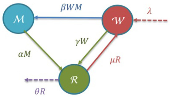
Figure 1.
Flow diagram of the waste plastic management.
Thus, the WPM is stated through the following three differential equations with quadratic nonlinearity system given by [23]
where . Along with (1), the given initial conditions are
In the model (1), the three constants are the initial amounts of the variables , , and at the beginning, which are non-negative.
In this work, we first analyze stability properties of the WPM system (1) from the viewpoint of dynamical system. To this end, the existence of two equilibria of this nonlinear dynamic systems are obtained in the first place. Then, we utilize the next-generation method to find the basic reproduction number of the system. Hence, by imposing some reasonable conditions on this number we prove that the given system is locally asymptotically stable at each equilibrium point.
To solve (1) numerically, we propose a novel collocation approach using a shifted version of the known Morgan-Voyce polynomials. Collocation techniques have been widely used through the use of different bases including Legendre, Chebyshev, Bernoulli, Bessel, Genocchi, Lucas, and Vieta–Fibonacci polynomials, see [24,25,26,27]. Each of these polynomials has its own set of parameters and orthogonality properties that help us to prove their convergence whenever they are used in the approximation procedures. In this paper, we investigate the application of the shifted Morgan-Voyce (SMV) polynomials for simulating system (1). The MV polynomials are related to the well-known Fibonacci polynomials and were first introduced in 1960 [28] and ever since the MV polynomials have been widely used for solving different real-life problems with complex geometry. For example, the MV polynomial has been used for simulating the delay integral differential equations in [29]. In addition, the authors in [30] adapted a matrix collocation technique with the aid of the MV polynomials for simulating the nonlinear ordinary differential equations with cubic and quadratic nonlinearity. To the best of our knowledge, this is the first attempt toward solving such a model by the shifted MV polynomials, and with the efficiency of the use of such polynomials, we were interested to see how this novel technique shall deal with such a problem. In order to get rid of the nonlinearity of WPM (1), we employ the quasilinearization method (QLM) combined to SMV collocation approach, which is more efficient than the direct approach. Another novelty of this paper is that the convergence analysis of SMV functions are established in two norms rigorously.
This content of this research paper is organized as follows: We introduce the details of the MV polynomials of the second kind in Section 2. Then, the uniform convergence analysis of SMV series is carried out. In Section 3, the direct SMV collocation approach is developed and then used to solve the presented model. Section 4 is devoted to the combined QLM-SMV approach based on the quasilinearization and collocation technique. The accuracy of the proposed techniques is tested through the calculation of the residual error analysis in Section 3 and Section 4. The numerical results are illustrated in Section 5. Furthermore, some comparisons are made with the outcomes of ode45 and the results of an available existing computational scheme. The conclusion of the study is summarized in Section 6. In Appendix A, we calculate the equilibrium points, the basic reproduction number and discuss the locally asymptotic stability of each equilibrium point.
2. The Shifted Morgan-Voyce Functions and Their Convergence Results
Here, in the first part, we review the definition of the original second-kind Morgan-Voyce (MV) functions and review some main properties of them. The shifted version of these polynomial is then introduced. The convergence analysis of shifted MV functions is established finally.
2.1. The Main Ingredients of Morgan-Voyce Functions: A Shifted Version
The second-kind of Morgan-Voyce (MV) polynomials are defined by [28,31]
for . For , we clearly obtain . By setting , we use the trigonometric relation to arrive at . In order to obtain the rest of MV polynomials for , it is sufficient to expand , which gives us the following recurrence
In addition, one may write them in an explicit representation form as
One can check that these polynomial functions are the (unique) solutions of the following differential equations
Let us derive the orthogonality property of the MV functions of the second kind. It is just mentioned in [31] that the set of MV functions are orthogonal with regard to for .
Lemma 1.
The set of MV polynomials are orthogonal with respect to weighting function on ,
Proof.
By utilizing the change of variable one can easily seen that and . Thus, we obtain . Thus, we have
We now simplify the terms and exploit the trigonometric relations to render
The result is obviously zero when we take . In contrast to this, for the result of integral is not zero and is equal to . Thus, the proof is completed. □
The locations of zeros of the second kind MV polynomial are determined in the following Lemma. They are all on , see [28].
Lemma 2.
The roots of of degree q are all distinct, real, and negative given by
In real applications, we are mainly interested in utilizing of the MV functions on an arbitrary interval . Therefore, the shifted MV polynomials are considered next:
Definition 1.
The shifted MV functions (SMVFs) on will be denoted by and are defined as
In the explicit form, they are given by
where .
According to (7), it is not a difficult task to prove that the set of shifted MV polynomials are orthogonal with regard to weight function . It is sufficient to utilize the change of variable (9) in the orthogonality condition (7). The resulting relation is
where represents the Kronecker delta function, which is if , and is zero otherwise. It is also interesting to specify the locations of zeros associated with SMV functions.The proof of the next result is given in Appendix B and is based on Lemma 2 and Definition 1.
Lemma 3.
All roots of the shifted MV functions are located inside defined by
where are given in (8). These points will be utilized as the collocation points in our algorithm, below.
Finally, let us consider the transformed SMV differential equation. Based on the given change of variable, the new equation can be obtained via (6) given by
2.2. Convergent and Error Analysis
Our goal now is to establish the convergence of the SMVFs of the second kind. Any function can be expressed as a linear of combination of SMVFs. Therefore, we write
By virtue of orthogonality relation (11), it is concluded that the coefficients , can be written in the form
In order to show that the series solution (13) is uniformly convergent, we need to estimate the coefficients . The following Theorem provides an upper bound for these coefficients.
Theorem 1.
Proof.
By utilizing the substitution , where in (14) one obtains
By using and the assumption on the second derivative we claim that
We now estimate the integral term in (18). By utilizing the change of variables , for we obtain
It can be clearly observed that for an odd , the value of integral is zero. On the other hand, for an even we have
An easy calculation shows that
Note that the inequality is true for all . Thus, we obtain
In practice, we take a finite series solution to approximate rather than an infinite series solution given in (13). This implies that we cut this series solution and take only SMVFs as
We proceed by defining the error between two consecutive approximations and . We will denote it by and is defined by
In addition, we use to denote the weighted norm on with regard to weight function . An error estimation for the error in the weighted norm is given in the next Theorem.
Theorem 2.
Under the assumptions of Theorem 1, the following error estimate his valid
where the constant C is defined in (15).
Proof.
According to the definition of error and (20) we obtain
It is now sufficient to use the orthogonality condition (11) and the result of Theorem 1 to obtain
□
Finding an upper bound for (global) error between the infinite series expansion of in (13) and its cut series solution in (20) is performed next. To this end, we define . We first prove the result in the weighted norm.
Theorem 3.
Proof.
Utilizing the orthogonality condition (11) reveals that
By employing the inequality (15) given in Theorem 3 to the former equality to obtain
Now, the well-known Integral Test from calculus gives us [32]
We finally insert the former inequality into (22). By taking the square root, the proof is accomplished. □
In order to obtain an error estimate for the global error (21) in the norm, the following Lemma is required.
Lemma 4.
The following upper bound for the SMV functions holds for all
Proof.
Here, represents the Chebyshev functions of the second kind. Furthermore, we know that [33]
Now the proof is straightforward by changing of variable and then taking the absolute values. □
Theorem 4.
3. The SMV Matrix Approach
We continue by writing the WPM system (1) in the following matrix form
Here, denotes the nonlinear term in (1) and we have utilized the following vectors and matrix
The aim is to approximate the unknown solutions as a combination of cutted SMV series solutions (20) with ()-terms. Thus, we have
Below, we seek the unknown coefficients for through a matrix collocation technique based on SMVFs. To proceed, we state the following Lemma, proof of which is straightforward.
Lemma 5.
Next Lemma provides a decomposition for the vector .
Lemma 6.
The vector of SMVFs can be decomposed as
where is the vector of shifted monomials and is an upper triangular matrix given by
Proof.
The proof is straightforward in view of relation (10) in Definition (1). It is sufficient to multiply the matrix by from the left. □
It should be noted that this matrix is non-singular as one can easily observe that . An immediate consequence of combining the results of two former Lemmas (two relations (27) and (28)) to arrive at
A simple calculation shows that
It follows that the derivatives of the cut series solutions in (29) can be written as
Lemma 7.
Proof.
To continue, one needs a set of collocation points on . One possible choice is to employ the roots of SMVFs given in (12). Clearly, we have unknowns for each solution in (26). Therefore, we consider the zeros of on . For convenience, we label these zeros as and will denote them by
The following result is obtained by placing the foregoing SMV nodes into the matrix form (25) of the WPM system (1) as
Lemma 8.
(b) Similarly, the matrix forms of relations (33) at the SMV nodes (34) are given by
where the matrix is defined by
Here, the matrices , the vector are already defined in (33).
In the next Lemma, we provide a matrix representation form for the nonlinear expression .
Lemma 9.
Proof.
The proof is relied on the following matrix representation
Now, it is sufficient to use the relations (26) for and . □
Ultimately, the so-called fundamental matrix equation will be constituted by placing the foregoing relations (35) and (37) into (36). It has the following form
where
It can be noticed that the former matrix Equation (39) is a nonlinear system comprising of unknowns for and to be found as the SMV coefficients. However, this nonlinear system is incomplete, since we have not yet taking the initial conditions (2) into account. Next, we will consider this task.
3.1. Converting the Initial Conditions into Matrix Form
Let us continue by entering the initial conditions (2) into the matrix Equation (39). First, we consider the matrix form (33) for the approximate solution . Now, it suffices to tend to obtain
Here, the constants and are known from (2). The replacement of three rows of matrix will be carried out next by the row matrices . The new fundamental matrix equation will be denoted by
Therefore, through solving the modified algebraic nonlinear system (40), we obtain the unknown SMV coefficients. The solution of this nonlinear system can be obtained utilizing any nonlinear solver such Newton type methods. After finding the vector , all unknowns , for , and as the coefficients in the expansion series (26) are determined. Thus, we obtain an approximate solution of model (1).
3.2. Error Estimation via REFs
As we mentioned earlier, it is very difficult to find the exact true solution of WPM system (1). This implies that one needs some alternative tools to measure the quality of approximate solutions proposed by our direct SMV collocation matrix method. One possible strategy is to estimate the achieved error via technique of residual error functions (REFs). So, it is sufficient to insert the -truncated series solutions (26) into the WPM system (1). Thus, we define the -truncated REFs related to (1) as
4. The Methodology of QLM-SMV
A description of the direct SMV-collocation approach applied to WPM system (1) is already conducted in the last section. However, a disadvantage of this approach is that we have to solve a non-linear system of equations. In fact, to gain more accuracy one needs to increase Q. In this case, the convergence of invoked non-linear algorithm usually does not takes place in a reasonable time or even we have not such convergence at all. As a remedy, one has to adopt the technique of quasi-linearization to convert the non-linear WPM system (1) into a family of linearized systems of equations. Starting from a rough first approximation, the method converges quadratically to the solution of the original problem (1).
Below, we will describe the main idea behind the quasilinearization method (QLM). Once the original non-linear model problem (1) is converted into a family of linear problems, we will employ the direct SMV matrix collocation procedure to each linearized equation. Below, this combined technique is called QLM-SMV. For more detailed information on QLM, we refer to [34,35,36].
Let the rough first approximation to is denoted by . The, the QLM for (42) reads
Note, along with former equations, we have the same initial conditions as (2). We also used the symbol to denote the corresponding Jacobian matrix. After some calculations, the applied QLM for the given model (42) has the following representation
where
According to (2), the supplemented initial conditions are given by
Now, we are in a position to solve the family of linearized Equation (43). In an analogue way as in the direct SMV matrix collocation procedure, we let the approximate solutions of this system can be expressed as a cut series with bases as
Concisely speaking, we now insert the SMV nodes (34) into (43). Utilizing the following matrix and vectors
and by using the relations (37) the following linear fundamental matrix equation is obtained
This can be equivalently rephrased as follows
Here, the matrices , , and are defined in (33) and
According to what we have discussed in the previous section, one requires to implement the initial condition in the matrix form and then enter into the fundamental matrix Equation (45). Let us the resulting modified system denoted by
By solving (46), we obtain the unknown coefficients for and . Note that in practice usually taking is sufficient to attain an accurate result as the solution obtained via direct SMV approach (40). However, the QLM-SVM technique is more efficient and consumes less computational time than the direct approach (40) as we show in the numerical section, below.
Similar to relations (41), the obtained approximate solutions (44) will be substituted into (1) to arrive at the following REFs
Note, these REFs can be used in the QLM-SMV approach to measure the accuracy of the obtained solutions of WPM system (1).
5. Numerical Experimental Results
Here, we intend to apply two proposed matrix algorithms based on SMVFs to the WPM system (1). In this respect, three set of parameters are considered to show the performance of these techniques. Various numerical simulations are performed to show the efficiency of the proposed collocation methods. The platform of simulations is Matlab software version 2021a.
The QLM parameter is chosen in the computational results, below. In the QLM-SVM, we use the initial approximation as the initial condition (2). A comparison with only available numerical model, i.e., the advanced numerical artificial neural network (ANN) technique described in [23]. As in [23], the following initial conditions in (2) are taken
We further use the Matlab function ode45 to validate our results.
Test 1.
To begin our computations, we let . Using the direct SMV collocation matrix technique we obtain
Similarly, by employing the QLM-SMV using iterations, the following approximate solutions are obtained on as
It can be readily seen that the coefficients of each pair of solutions are approximately coincided up to five or six digits. To further justify, we plot all the above approximations in Figure 2. We also validate our obtained results by comparing the solutions with the outputs of the well-known Matlab function, i.e., ode45 as shown in Figure 2.
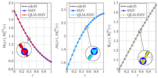
Figure 2.
Comparisons of numerical solutions obtained via SMV/QLM-SMV in Test Case 1 with .
The corresponding REFs corresponding to are visualized in Figure 3. Since the accuracy of both approaches are the same for different values of Q, we just consider the QLM-SMV and the related achieved REFs obtained via (47). Figure 3 displays the REFs for diverse values of . Let us compare our results in terms of the achieved errors in Test case 1 with the corresponding results obtained via ANN in [23]. In Figure 14a–c of [23], the absolute errors (AE) related to three solutions , , and were visualized. However, it is not known how the authors in [23] obtained such results. The achieved AE for these three solutions are in the ranges , , and , respectively. Obviously, our obtained results with are comparable with the outcomes of ANN. However, our method with simple implementation than ANN produces results within the desired level of accuracy by just increasing Q as shown in Figure 3.
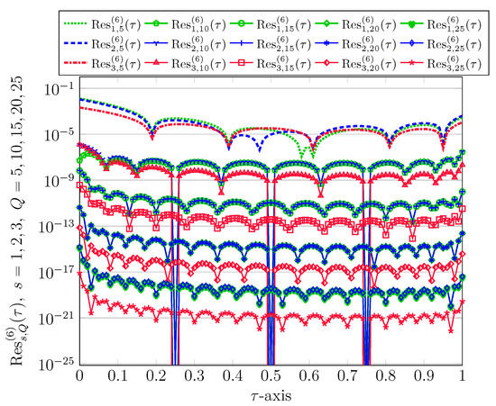
Figure 3.
Comparisons of achieved REFs via QLM-SMV in Test Case 1 with .
Besides the visualizations we have plotted in Figure 2 and Figure 3 for the first Test Case (1), we also report the numerical results together with related REFs in both SVM and QLM-SVM collocation techniques in Table 1, Table 2 and Table 3. Using , we tabulate the results related to of WPM system (1) in these tables. For comparisons, the outputs of ode45 are also given at some points . Obviously, our results are accurate enough and by increasing Q we obtain more accuracy as shown in the previous Figure 3 graphically.

Table 1.
The comparison of numerical results for in SMV/QLM-SMV procedure using in Test Case 1.
Table 2.
The comparison of numerical results for in SMV/QLM-SMV procedure using in Test Case 1.
Table 3.
The comparison of numerical results for in SMV/QLM-SMV procedure using in Test Case 1.
Again, we emphasize that the QLM-SMV technique is more efficient than SVM matrix method especially when Q is becoming large. To show an evidence, we measure the elapsed times needed to solve the fundamental matrix Equations (40) and (46). For , the required CPU time to solve it via SMV approach is s while the consumed time is only s when solving the () sequence of linear matrix equations via QLM-SMV. Obviously, the latter matrix collocation approach is effective about a factor of 20. This factor will be drastically increased by increasing the number of bases.
Test 2.
As the second test case, we consider the following parameters for the WPM system (1) taken from [23]
We take for this example. By utilizing the direct SVM collocation strategy we obtain the following approximate solutions
Figure 4 displays the graphics of the forgoing approximate solutions on the interval along with the related REFs namely for . Note also that we have plotted the related solutions obtained via ode45 to validate our results as show by dashed lines.
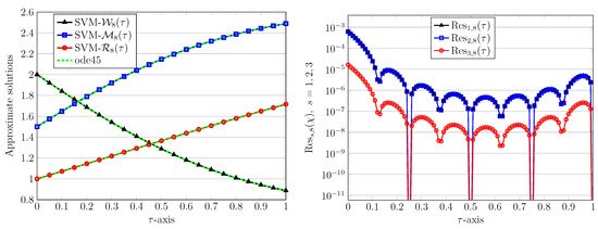
Figure 4.
Graphics of numerical solutions obtained via SMV technique (left) and related REFs (right) in Test Case 2 with .
The numerical convergence of the proposed collocation approaches is investigated next. For this purpose, we employ QLM-SMV with various . The results of REFs for these values are shown in Figure 5. It can be obviously observed that by increasing Q we obtain the desired level of accuracy. In an analogue way as in Test Case 1 we compare our results in terms of the achieved errors in Test Case 2 with the real outcomes obtained via ANN in [23]. In Figure 14a–c of [23], the reported AE associated with the three solutions , , and are in the ranges , , and , respectively. Consequently, our achieved REFs with are comparable with the those obtained by ANN. It can be seen from Figure 5 that we can gain more accurate results by increasing Q.
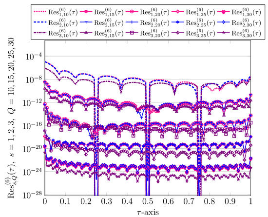
Figure 5.
Comparisons of achieved REFs via QLM-SMV in Test Case 2 with .
Some precise comparisons are also made in Table 4, Table 5 and Table 6 for the second Test Case. Similar to the previous example, we utilize here. The outcomes of the method ode45 are reported in these tables for validation. It should be noted that the maximum value of REFs is occurred at the initial conditions for all three solutions as one sees from the former figures.
Table 4.
The comparison of numerical results for in SMV/QLM-SMV procedure using in Test Case 2.
Table 5.
The comparison of numerical results for in SMV/QLM-SMV procedure using in Test Case 2.
Table 6.
The comparison of numerical results for in SMV/QLM-SMV procedure using in Test Case 2.
We next go beyond the unit interval and take a relatively large interval . The approximate solutions obtained by using the QLM-SMV and with bases are presented in Figure 6. Plotting further solutions obtained by ode45 show that our results are in good alignment with them. The related REFs are displayed in Figure 7. From the parameters given in the second test problem we find that the values of the basic reproduction number in (A4) and the second equilibrium point in (A3) become
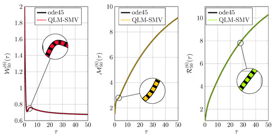
Figure 6.
Comparisons of numerical solutions obtained via QLM-SMV in Test Case 2 with .
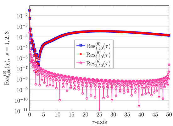
Figure 7.
Graphics of achieved REFs via QLM-SMV in Test Case 2 with .
By looking at the plots we can infer that the approximate solutions converge to the stable point as .
Let us finally investigate the effectiveness and high-order accuracy of our proposed QLM-SMV procedure through computing the errors in the norm. For a fixed d, we calculate the maximum values of the REF norm of the solutions , and by
for , where the REFs are defined in (47). To justify the theoretical findings and in order to the check the numerical order of convergence of the QLM-SMV, we compute the following expressions
The results of error norms and the related order of convergences for two Test Case 1 and 2 are tabulated in Table 7. Here, we have used and various , . By looking at Table 7, it can be seen that the behavior of the obtained order of convergences is exponentially similar. This confirms the high-order accuracy of the QLM-SMV approach.
Table 7.
The results of norms, the corresponding convergence rate in Test Case 1 and 2 using the QLM-SMV procedure with diverse Q and .
6. Conclusions
In this manuscript, we have described two accurate matrix collocation techniques based on the (novel) shifted Morgan-Voyce (SMV) functions to find the approximate solutions to a nonlinear system of differential equations arising in modeling of waste plastic management. From theoretical point of view, the existence and the stability properties of equilibrium points of the underlying system are investigated based on the basic reproduction number . From numerical perspectives, we first employ the SMV matrix collocation approach to solve this system accurately. In the second approach, we first convert the given nonlinear system into a family of linearized systems followed by applying the SMV collocation technique to them efficiently. Through a comprehensive error analysis we proved that the SMV expansion series is convergent in the weighted and norms. Numerical simulations using various model parameters are presented to show the accurateness as well as the effectiveness of the proposed collocation techniques. We compare our results with those obtained via ANN [23] to validate the accuracy of the proposed techniques. In conclusion, our second presented QLM-SMV technique produces comparable accurate results in comparison with the direct SVM approach. Furthermore, the calculations involved in QLM-SMV are simple, straightforward, and have a lower computation cost.
Author Contributions
Conceptualization, M.I., M.P. and W.A.; methodology, M.I. and M.P.; software, M.I.; validation, M.I., M.P. and W.A.; formal analysis, M.I. and M.P.; funding acquisition, M.I. and W.A.; investigation, M.I., M.P. and W.A.; writing—original draft preparation, M.I., M.P. and W.A.; writing—review and editing, M.I., M.P. and W.A. All authors have read and agreed to the published version of the manuscript.
Funding
This research received no external funding.
Institutional Review Board Statement
Not applicable.
Informed Consent Statement
Not applicable.
Data Availability Statement
No data was used for the research described in the article.
Acknowledgments
The authors would like to thank the anonymous Reviewers and Editor for providing helpful comments and suggestions which further improved this work.
Conflicts of Interest
The authors declare no conflict of interest.
Appendix A. Properties and Stability of the Model
In the part, we first derive the equilibrium points of the given WPM model (1). Hence, the basic reproduction number related to this system is obtained. Next, we investigate the stability of two equilibrium points and establish some results.
Appendix A.1. Equilibria and Basic Reproduction Number of the Model
The equilibria of the model (1) are obtained by solving the following equations:
The system has two solutions: When , the equilibrium is obtained as follows
and when , the equilibrium point is
The basic reproduction number can be obtained as dominant eigenvalue of the next generation matrix [37]. Using this method, we write the second equation in (A1) as
where and . By letting and , the basic reproduction number related to this model is given by
For the equilibrium in which , we have
Thus, we have if and only if . Hence, based on the former discussion we can state the following Lemma:
Lemma A1.
Model (1) has only the equilibrium (corresponding to ) when and it also has a unique equilibrium (corresponding to ) if .
Appendix A.2. Stability of the Model
For studying the local stability of the equilibria of the model (1), we consider the eigenvalues of the Jacobian matrix at each equilibrium point. The equilibrium is stable if and only if the eigenvalues of the related Jacobian matrix have negative real part. The Jacobian matrix of the model (1) at has the following representation
At equilibrium we have
and its eigenvalues are , which is negative if and only if . Other eigenvalues of are the eigenvalues of the following matrix
By the Routh–Hurwitz criterion [38], the real part of eigenvalues of matrix S are negative if and only if and . However, we have
Thus, all eigenvalues of have negative real part and stability of the model at is concluded.
Theorem A1.
At equilibrium we have and thus we obtain.
It can be easily seen that
The next observation is
Moreover, we have
Theorem A2.
Proof.
According to Routh–Hurwitz criterion [38], the roots of the characteristic polynomial of the Jacobian matrix J lie in the left half of the Cartesian plane if and only if , , and , where
From preceding calculations (A10) and (A11) for matrix in (A9) we observe clearly that and . Moreover, we have
Thus, the proof is completed. □
Appendix B
Proof of Lemma 3
On account of Lemma 2, the zeros of are denoted by . Therefore, we can express in terms of its roots as follows
It should emphasize that the leading coefficient of the original MV function is always one in accordance to their definition (5). Now, we use the change of variable (9) to arrive at
By equating the former equation to zero we find that the roots are for . Thus, the proof is complete. □
References
- Argüello, G. Marine Pollution, Shipping Waste and International Law; Routledge: London, UK, 2019. [Google Scholar]
- Dabrowska, J.; Sobota, M.; Swiader, M.; Borowski, P.; Moryl, A.; Stodolak, R.; Kucharczak, E.; Zieba, Z.; Kazak, J.K. Marine waste-sources, fate, risks, challenges and research needs. Int. J. Environ. Res. Public Health 2021, 18, 433. [Google Scholar] [CrossRef] [PubMed]
- Jambeck, J.R.; Geyer, R.; Wilcox, C.; Siegler, T.R.; Perryman, M.; Andrady, A.; Narayan, R.; Law, K.L. Plastic waste inputs from land into the ocean. Science 2015, 347, 768–771. [Google Scholar] [CrossRef] [PubMed]
- Murray, F.; Cowie, P.R. Plastic contamination in the decapod crustacean Nephrops norvegicus (Linnaeus, 1758). Mar. Pollut. Bull. 2011, 62, 1207–1217. [Google Scholar] [CrossRef] [PubMed]
- Ynet. The United Nations Environment Program Reports that 85 Percent of Ocean Debris is Plastic. 2021. Available online: https://t.ynet.cn/baijia/31615238.html (accessed on 20 November 2022).
- Almroth, B.C.; Eggert, H. Marine plastic pollution: Sources, impacts, and policy issues. Rev. Environ. Econ. Policy 2019, 13, 317–326. [Google Scholar] [CrossRef]
- Marks, D.; Miller, M.A.; Vassanadumrongdee, S. The geopolitical economy of Thailand’s marine plastic pollution crisis. Asia Pac. Viewp. 2020, 61, 266–282. [Google Scholar] [CrossRef]
- Sulis, G.; Sayood, S.; Gandra, S. Antimicrobial resistance in low-and middle-income countries: Current status and future directions. Expert Rev.-Anti-Infect. Ther. 2022, 20, 147–160. [Google Scholar] [CrossRef]
- Wu, H.H. A study on transnational regulatory governance for marine plastic debris: Trends, challenges, and prospect. Mar. Policy 2020, 136, 103988. [Google Scholar] [CrossRef]
- Zhang, C.; Guo, L.; Luo, Q.; Wang, Y.; Wu, G. Research on marine plastic garbage governance in Northwest Pacific Region from the perspective of cooperative game. J. Clean. Prod. 2022, 354, 131636. [Google Scholar] [CrossRef]
- Louzoun, Y.; Xue, C.; Lesinski, G.B.; Friedman, A. A mathematical model for pancreatic cancer growth and treatments. J. Theor. Biol. 2014, 351, 74–82. [Google Scholar] [CrossRef]
- Khajanchi, S. The impact of immunotherapy on a glioma immune interaction model. Chaos Solit. Fract. 2021, 152, 111346. [Google Scholar] [CrossRef]
- Lazebnik, T.; Aaroni, N.; Bunimovich-Mendrazitsky, S. PDE based geometry model for BCG immunotherapy of bladder cancer. Biosystems 2020, 200, 104319. [Google Scholar] [CrossRef]
- Gude, V. Modeling a decision support system for COVID-19 using systems dynamics and fuzzy inference. Health Inform. J. 2022, 28, 14604582221120344. [Google Scholar] [CrossRef] [PubMed]
- Shtilerman, E.; Thompson, C.J.; Stone, L.; Bode, M.; Burgman, M. A novel method for estimating the number of species within a region. Proc. Royal Soc. B Biol. Sci. 2014, 281, 20133009. [Google Scholar] [CrossRef] [PubMed]
- Shaikh, A.; Nisar, K.S.; Jadhav, V.; Elagan, S.K.; Zakarya, M. Dynamical behaviour of HIV/AIDS model using fractional derivative with Mittag-Leffler kernel. Alex. Eng. J. 2022, 61, 2601–2610. [Google Scholar] [CrossRef]
- Yüzbası, S.; Izadi, M. Bessel-quasilinearization technique to solve the fractional-order HIV-1 infection of CD4+ T-cells considering the impact of antiviral drug treatment. Appl. Math. Comput. 2022, 431, 127319. [Google Scholar] [CrossRef]
- Iqbal, Z.; Ahmed, N.; Baleanu, D.; Adel, W.; Rafiq, M.; Rehman, M.A.; Alshomrani, A.S. Positivity and boundedness preserving numerical algorithm for the solution of fractional nonlinear epidemic model of HIV/AIDS transmission. Chaos Solit. Fract. 2020, 134, 109706. [Google Scholar] [CrossRef]
- Elsonbaty, A.M.R.; Sabir, Z.; Ramaswamy, R.; Adel, W. Dynamical analysis of a novel discrete fractional SITRS model for COVID-19. Fractals 2021, 29, 2140035. [Google Scholar] [CrossRef]
- Baleanu, D.; Abadi, M.H.; Jajarmi, A.; Vahid, K.Z.; Nieto, J.J. A new comparative study on the general fractional model of COVID-19 with isolation and quarantine effects. Alex. Eng. J. 2022, 61, 4779–4791. [Google Scholar] [CrossRef]
- Aguiar, M.; Anam, V.; Blyuss, K.B.; Estadilla, C.D.; Guerrero, B.V.; Knopoff, D.; Kooi, B.W.; Srivastav, A.K.; Steindorf, V.; Stollenwerk, N. Mathematical models for dengue fever epidemiology: A 10-year systematic review. Phys. Life Rev. 2022, 40, 65–92. [Google Scholar] [CrossRef]
- Izadi, M.; Yüzbası, S.; Adel, W. Accurate and efficient matrix techniques for solving the fractional Lotka–Volterra population model. Phys. A 2022, 600, 127558. [Google Scholar] [CrossRef]
- AL-Nuwairan, M.; Sabir, Z.; Raja, M.A.Z.; Aldhafeeri, A. An advance artificial neural network scheme to examine the waste plastic management in the ocean. AIP Adv. 2022, 12, 045211. [Google Scholar] [CrossRef]
- Fathy, M.; El-Gamel, M.; El-Azab, M.S. Legendre–Galerkin method for the linear Fredholm integro-differential equations. Appl. Math. Comput. 2014, 243, 789–800. [Google Scholar] [CrossRef]
- Atta, A.G.; Youssri, Y.H. Advanced shifted first-kind Chebyshev collocation approach for solving the nonlinear time-fractional partial integro-differential equation with a weakly singular kernel. Comput. Appl. Math. 2022, 41, 381. [Google Scholar] [CrossRef]
- Adel, W.; Sabir, Z. Solving a new design of nonlinear second-order Lane–Emden pantograph delay differential model via Bernoulli collocation method. Eur. Phys. J. Plus. 2020, 135, 427. [Google Scholar] [CrossRef]
- Izadi, M.; Yüzbası, S.; Ansari, K.J. Application of Vieta-Lucas series to solve a class of multi-pantograph delay differential equations with singularity. Symmetry 2021, 13, 2370. [Google Scholar] [CrossRef]
- Swamy, M.N.S. Properties of the polynomials defined by Morgan-Voyce. Fibonacci Quart. 1966, 4, 73–81. [Google Scholar]
- Özel, M.; Tarakci, M.; Sezer, M. Morgan-Voyce polynomial approach for ordinary linear delay integro-differential equations with variable delays and variable bounds. Hacettepe J. Math. Stat. 2021, 50, 1434–1447. [Google Scholar]
- Tarakci, M.; Özel, M.; Sezer, M. Solution of nonlinear ordinary differential equations with quadratic and cubic terms by Morgan-Voyce matrix-collocation method. Turk J. Math. 2020, 44, 906–918. [Google Scholar] [CrossRef]
- Swamy, M.N.S. Further properties of Morgan-Voyce polynomials. Fibonacci Quart. 1968, 6, 167–175. [Google Scholar]
- Stewart, G.W. Afternotes on Numerical Analysis. SIAM 1996, 49, 157. [Google Scholar]
- Mason, J.; Handscomb, D. Chebyshev Polynomials; Chapman and Hall: New York, NY, USA; CRC: Boca Raton, FL, USA, 2003. [Google Scholar]
- Izadi, M. An approximation technique for first Painlevé equation. TWMS J. App. Eng. Math. 2021, 11, 739–750. [Google Scholar]
- Izadi, M.; Yüzbası, S.; Noeiaghdam, S. Approximating solutions of non-linear Troesch’s problem via an efficient quasi-linearization Bessel approach. Mathematics 2021, 9, 1841. [Google Scholar] [CrossRef]
- Izadi, M.; Srivastava, H.M. Generalized Bessel quasilinearlization technique applied to Bratu and Lane-Emden type equations of arbitrary order. Fractal Fract. 2021, 5, 179. [Google Scholar] [CrossRef]
- Van den Driessche, P.; Watmough, J. Reproduction numbers and sub-threshold endemic equilibria for compartmental models of disease transmission. Math. Biosci. 2002, 180, 29–48. [Google Scholar] [CrossRef] [PubMed]
- Ortega, J.M. Matrix Theory: A Second Course; Springer: New York, NY, USA, 2013. [Google Scholar]


Publisher’s Note: MDPI stays neutral with regard to jurisdictional claims in published maps and institutional affiliations. |
© 2022 by the authors. Licensee MDPI, Basel, Switzerland. This article is an open access article distributed under the terms and conditions of the Creative Commons Attribution (CC BY) license (https://creativecommons.org/licenses/by/4.0/).