Constructing a Linearly Ordered Topological Space from a Fractal Structure: A Probabilistic Approach

Abstract

Recent studies have shown that it is possible to construct a probability measure from a fractal structure defined on a space. On the other hand, a theory on cumulative distribution functions from an order on a separable linearly ordered topological space has been developed. In this paper, we show how to define a linear order on a space with a fractal structure, so that these two theories can be used interchangeably in both topological contexts.

1. Introduction

Fractal structures were introduced in [1] in order to study non-Archimedean quasimetrization, although they have a wide range of applications. Some of these applications can be found in [2] and include metrization, topological and fractal dimension, filling curves, completeness, transitive quasi-uniformities and inverse limits of partially ordered sets.

In recent studies, the authors proposed a way to construct probability measures on spaces with a fractal structure by taking advantage of its recursive nature. For this topic, we refer the reader to [3,4], although it is convenient to have a look at [5], which is about the completion of a space with a fractal structure, a key element in this construction. The idea is starting from a pre-measure defined on the elements of the fractal structure, or the topological structures induced by it, and looking for conditions so that methods on the construction of outer measures are used to build a probability measure on the original space as an extension of the pre-measure. An alternative way to relate probability measures with fractals can be found, for example, in [6], which deals with the calculation of the relative multifractal Hausdorff and packing dimensions of measures in a probability space.

On the other hand, in [7,8,9], the authors developed a theory about the cumulative distribution function of a probability measure on a linearly ordered topological space. More precisely, in [7], it is shown that the cumulative distribution function of a probability measure on a separable linearly ordered topological space satisfies some properties which are similar to those that are well-known in the classical theory (when working on the real line). Moreover, in that paper, a definition of the inverse of a cumulative distribution function is given for the case in which the space is compact, which can be used to generate samples of the distribution and to calculate integrals with respect to the measure. Next, in [8], it is proved that each cumulative distribution function on a separable linearly ordered topological space can be extended to the Dedekind–MacNeille completion of the space, where it does make sense to define its pseudo-inverse, even if the base space is not compact. Recall that, when working with probability measures on the reals, using a cumulative distribution function is quite handy when trying to describe the probability measure. Moreover, it is well known that in the classical theory of probability measures and cumulative distribution functions, there is a one-to-one relationship between these two mathematical tools (see [10]). Indeed, in [9], the authors showed that this relationship holds in the context of linearly ordered topological spaces, not only between a probability measure and its cumulative distribution function, but also between a probability measure and the pseudo-inverse of its cumulative distribution function. Cumulative distribution functions have also been used, in the most recent literature, to generate fuzzy numbers, for which we refer the reader to [11].

Now, once we know how to construct probability measures on a space with a fractal structure and have studied the whole theory on cumulative distribution functions when working on a separable linearly ordered topological space, the next step is trying to connect both theories. For example, in [12], it was shown that a cumulative distribution function can be constructed from the invariant Borel probability measure associated with the iterated function system of a Cantor set; see also ([3], Def. 4.12) in order to know how to construct a fractal structure on the attractor of an iterated function system. In Section 3, given a space with a fractal structure (and, more generally, an ultrametric space), we can define an order under some compatibility conditions such that the Borel $\sigma$-algebras of both topologies (the one given by the ultrametric and the one given by the order) coincide. In fact, that compatibility condition and the relationship between the topologies are given in Section 3.1. Indeed, in Section 3.2 and Section 3.3, we show two examples of linear orders that can be constructed and study their properties. Once we have a linear order on a space with a fractal structure, we show how a pre-measure and a cumulative distribution function can be related, so we study two situations. The first is when a cumulative distribution function of a probability measure is given. Then, it is shown how a pre-measure can be defined such that the cumulative distribution function of the corresponding probability measure is the original one (see Section 3.4). The second is when a pre-measure is given. Then, it is shown how the cumulative distribution function of the probability measure constructed from the pre-measure (following the procedure exposed in [3,4]) can be described in terms of the pre-measure defined on the fractal structure (see Section 3.5). This relationship allows to move between pre-measures and cumulative distribution functions, so researchers can use the tool that best suits their needs.

2. Preliminaries

2.1. Fractal Structures

While it is true that fractal structures were introduced in [1] for a topological space, we will work with its definition on a set instead of a topological space, as it has been previously used in other works.

First, recall that a cover ${\Gamma }_2$ is a strong refinement of another cover ${\Gamma }_1$, written as ${\Gamma }_2\prec \prec {\Gamma }_1$, if ${\Gamma }_2$ is a refinement of ${\Gamma }_1$ (that is, each element of ${\Gamma }_2$ is contained in some element of ${\Gamma }_1$), denoted by ${\Gamma }_2\prec {\Gamma }_1$, and for each $B\in {\Gamma }_1$, it holds that $B=\bigcup \{A\in {\Gamma }_2:A\subseteq B\}$. The definition of a fractal structure is as follows.

Definition 1.

A fractal structure on a set X is a countable family of coverings $\mathsf{\Gamma }=\{{\Gamma }_n:n\in \mathbb{N}\}$ such that ${\Gamma }_{n+1}\prec \prec {\Gamma }_n$. The cover ${\Gamma }_n$ is called the level n of the fractal structure.

A fractal structure induces a transitive base of a quasi-uniformity given by $\{U_{{\Gamma }_n}:n\in \mathbb{N}\}$, where $U_{\Gamma }=\{(x,y)\in X\times X:y\notin \bigcup \{A\in \Gamma :x\notin A\}\}$ for each cover $\Gamma$.

Now let $\mathsf{\Gamma }=\{{\Gamma }_n:n\in \mathbb{N}\}$ be a fractal structure on a set X. For each $n\in \mathbb{N}$, we define $U_{xn}=U_{{\Gamma }_n}\left(x\right)=X\setminus {\bigcup }_{x\notin A,A\in {\Gamma }_n}A$, $U_{xn}^{-1}=U_{{\Gamma }_n}^{-1}\left(x\right)={\bigcap }_{x\in A,A\in {\Gamma }_n}A$ and $U_{xn}^{*}=U_{xn}\cap U_{xn}^{-1}$.

Let $d:X\times X\to {\mathbb{R}}_0^{+}$ be a function on X, where ${\mathbb{R}}_0^{+}$ denotes, as usual, the set of non-negative reals. Next, we include some properties of d for any $x,y,z\in X$ in order to characterize different types of distance functions.

• $d(x,x)=0$.
• $d(x,z)\le d(x,y)+d(y,z)$.
• $d(x,y)=d(y,x)$.
• $d(x,y)=0$ implies that $x=y$.
• $d(x,y)=0=d(y,x)$ implies that $x=y$.
• $d(x,z)\le max\left\{d\right(x,y),d(y,z\left)\right\}$.

Definition 2.

From the previous conditions, it is possible to define different kinds of distance functions as follows:

• One can say d is a metric on X if $1,2,3$ and 4 are satisfied.
• One can say d is a pseudometric on X if $1,2$ and 3 are satisfied.
• One can say d is a quasi-metric on X if $1,2$ and 4 are satisfied.
• One can say d is a quasi-pseudometric on X if 1 and 2 are satisfied.
• One can say d is a $T_0$-quasi-metric on X if $1,2$ and 5 are satisfied.
• One can say d is a dissimilarity on X if 1 and 2 are satisfied.

Moreover, if one of the previous distance functions satisfies 6, it will be called non-Archimedean. A non-Archimedean metric is also called an ultrametric.

The non-Archimedean quasi-pseudometric $d_{\Gamma }$ induced by $\Gamma$ is defined by (see [1])

$$d_{\Gamma }(x,y)=\left\{\begin{array}{ccc}\frac{1}{2^n}\hfill & if& y\in U_{xn}\setminus U_{x,n+1}\\ \\ 1\hfill & if& y\notin U_{x1}\\ \\ 0\hfill & & \mathrm{otherwise}\end{array}\right.$$

We will denote it simply by d if there is no confusion on the fractal structure $\mathsf{\Gamma }$.

First, note that $B(x,\frac{1}{2^n})=U_{x,n+1}$ and, also, that d satisfies the inequality $d(x,z)\le max\left\{d\right(x,y),d(y,z\left)\right\}$ for each $x,y,z\in X$, which gives us that d is a non-Archimedean quasi-pseudometric. In addition, we can consider the conjugate quasi-pseudometric, $d^{-1}(x,y)=d(y,x)$, and the supremum pseudometric, $d^{*}(x,y)=max\{d(x,y),d(y,x)\}$, which is a non-Archimedean pseudometric (or ultrapseudometric).

2.2. Completion of a Fractal Structure

In [5], the authors showed how to construct the bicompletion of a space with a fractal structure using a sequence of the inverse limit of posets. Let $(X,\mathsf{\Gamma })$, suppose that X is $T_0$ with respect to $d_{\mathsf{\Gamma }}$, and consider the collection $G_n=\{U_{xn}^{*}:x\in X\}$, which is a partition of X for each $n\in \mathbb{N}$. Then, we can define the projection ${\rho }_n:X\to G_n$ by ${\rho }_n\left(x\right)=U_{xn}^{*}$ and the bonding maps ${\varphi }_n:G_{n+1}\to G_n$ given by ${\varphi }_n\left({\rho }_{n+1}\left(x\right)\right)={\rho }_n\left(x\right)$. We will denote the inverse limit by $\tilde{X}=\underleftarrow{\lim }{G}_n=\{(g_1,g_2,\dots )\in {\prod }_{n=1}^{\infty }{G}_n:{\varphi }_n\left(g_{n+1}\right)=g_n,\forall n\in \mathbb{N}\}$. Now, we can define an embedding from X into $\tilde{X}$ by $\rho :X\to \tilde{X}$ defined by $\rho \left(x\right)={\left({\rho }_n\left(x\right)\right)}_{n\in \mathbb{N}}$. Next, we recall (see [5]) how to extend a fractal structure on X to a fractal structure on $\tilde{X}$. For that purpose, we define $\tilde{A}=\{{\left({\rho }_n\left(x_n\right)\right)}_{n\in \mathbb{N}}\in \tilde{X}:x_n\in A\}$ and $\tilde{\mathsf{\Gamma }}=\{{\tilde{\Gamma }}_n:n\in \mathbb{N}\}$, where ${\tilde{\Gamma }}_n=\{\tilde{A}:A\in {\Gamma }_n\}$, and we have that $\tilde{\mathsf{\Gamma }}$ is a fractal structure on $\tilde{X}$ (see ([5], Prop 4.3)). We denote by $\tilde{d}=d_{\tilde{\mathsf{\Gamma }}}$ the non-Archimedean quasi-pseudometric induced by $\tilde{\mathsf{\Gamma }}$ on $\tilde{X}$ and define, for each $n\in \mathbb{N}$, ${\tilde{U}}_{xn}=\tilde{X}\setminus {\bigcup }_{x\notin \tilde{A},\tilde{A}\in {\tilde{\Gamma }}_n}\tilde{A}=U_{{\tilde{\Gamma }}_n}\left(x\right)$, ${\tilde{U}}_{xn}^{-1}=\{y\in X:x\in {\tilde{U}}_{yn}\}$ and ${\tilde{U}}_{xn}^{*}={\tilde{U}}_{xn}\cap {\tilde{U}}_{xn}^{-1}$.

Moreover, in order to simplify the notations, we will make the identifications $\rho \left(A\right)\equiv A$ for $A\subseteq X$, $\rho \left(x\right)\equiv x$ for $x\in X$, $\rho \left(X\right)\equiv X$, $\rho \left(U_{xn}\right)=U_{xn}$ for $x\in X$ and $n\in \mathbb{N}$ and so on. The next proposition gathers some relationships between elements of X and their extensions to $\tilde{X}$.

Proposition 1

([5], Prop. 4.4).

1. 

$\tilde{A}\cap X=A$ for each $A\in {\Gamma }_n$ and $n\in \mathbb{N}$.

2. 

$\tilde{A}={\mathrm{Cl}}_{{\tilde{\tau }}^{*}}\left(A\right)$ for each $A\in {\Gamma }_n$ and $n\in \mathbb{N}$.

3. 

${\tilde{U}}_{xn}\cap X=U_{xn}$ for each $x\in X$ and $n\in \mathbb{N}$.

4. 

${\tilde{U}}_{xn}^{-1}\cap X=U_{xn}^{-1}$ for each $x\in X$ and $n\in \mathbb{N}$.

5. 

${\tilde{U}}_{xn}^{*}\cap X=U_{xn}^{*}$ for each $x\in X$ and $n\in \mathbb{N}$.

Finally, it is proven that $(\tilde{X},{\tilde{d}}^{*})$ is the completion of $(X,d^{*})$ (in [5], Prop 5.2). If we take into account that a quasi-pseudometric d is said to be bicomplete if the pseudometric $d^{*}$ is complete, we obtain, as an immediate consequence of the previous result that $(\tilde{X},\tilde{d})$ is the bicompletion of $(X,d)$.

2.3. Linearly Ordered Topological Spaces

First, we recall the definition of a linear order and a linearly ordered topological space.

Definition 3

([13], Chapter 1). A partially ordered set $(P,\le )$ (that is, a set P with the binary relation ≤ that is reflexive, antisymmetric and transitive) is totally ordered if every $x,y\in P$ is comparable, that is, $x\le y$ or $y\le x$. In this case, the order is said to be total or linear.

For a further reference about partially ordered sets, see, for example, [14]. Moreover, ref. [15] is a useful reference about ordered sets.

Definition 4

([16], Section 1). A linearly ordered topological space is a triple $(X,\tau ,\le )$, where $(X,\le )$ is a linearly ordered set and where τ is the topology of the order ≤.

The definition of the order topology is as follows.

Definition 5

([17], Part II, 39). Let X be a set which is linearly ordered by <. We define the order topology τ on X by taking the subbase $\left\{\right\{x\in X:x<a\}:a\in X\}\cup \left\{\right\{x\in X:x>a\}:a\in X\}$.

Given a linear order ≤ on X, we define the next sets.

Definition 6.

Let $a,b\in X$ with $a\le b$. We define the set $]a,b]=\{x\in X:a<x\le b\}$. Analogously, we define $]a,b[,[a,b]$ and $[a,b[$. Moreover, $(\le a)$ is given by $(\le a)=\{x\in X:x\le a\}$. $(<a),(\ge a)$, and $(>a)$ are defined similarly.

Definition 7.

Let $a\in X$. We will also use $]a,\infty [$ and $[a,\infty [$ to denote $(>a)$ and $(\ge a)$, respectively. Similarly, $]-\infty ,a[$ and $]-\infty ,a]$ will also denote $(<a)$ and $(\le a)$, respectively.

Definition 5 suggests the next one.

Definition 8

([7], Prop. 11). Given $x\in X$, it is said to be a left-isolated (respectively right-isolated) point if $(<x)=\varnothing$ (respectively $(>x)=\varnothing$) or there exists $z\in X$ such that $]z,x[=\varnothing$ (respectively, there exists $z\in X$ such that $]x,z[=\varnothing$). Moreover, we will say that $x\in X$ is isolated if it is both right and left-isolated.

There exists an equivalence between the property of the second countable for $\tau$ and the countability of the set of isolated points.

Proposition 2

([7], Prop. 5). Let X be a linearly ordered topological space. X is second countable with respect to the topology τ if and only if X is separable and the set of points which are right-isolated or left-isolated is countable.

We also need to recall the definition of a convex set.

Definition 9

([16], Section 1). A subset $C\subseteq X$ is said to be convex in X if, whenever $a,b\in C$ with $a\le b$, $\{x\in X:a\le x\le b\}$ is a subset of C.

Proposition 3

([7], Cor. 1). Let X be a separable linearly ordered topological space and $A\subseteq X$ be a convex subset. Then, it holds that:

1. 

If there exist both minimum and maximum of A, then $A=[minA,maxA]$.

2. 

If there does not exist the minimum of A but it does its maximum, then there exists a decreasing sequence $a_n\in A$ such that $A={\bigcup }_{n\in \mathbb{N}}]a_n,maxA]$.

3. 

If there does not exist the maximum of A, but its minimum does exist, then there exists an increasing sequence $b_n\in A$ such that $A={\bigcup }_{n\in \mathbb{N}}[minA,b_n[$.

4. 

If there does not exist the minimum of A nor its maximum, then there exists a decreasing sequence $a_n\in A$ and an increasing one $b_n\in A$ such that $A={\bigcup }_{n\in \mathbb{N}}]a_n,b_n[$.

Proposition 4

([7], Prop. 6). Let $x\in X$. Then x is not left-isolated (respectively, right-isolated) if and only if there exists a monotone sequence which left τ-converges (respectively, right τ-converges) to x.

2.4. Cuts and the Dedekind–MacNeille Completion

First, we recall the definition of a complete lattice.

Definition 10

([18], Def. 8.1, Section 8.1). Let L be a partially ordered set. Then, L is called a lattice if and only if any two elements of L have a supremum and an infimum. L is called a complete lattice if and only if any subset of L has a supremum and an infimum.

Definition 11

([18], Defs. 2.16, 2.17). Let P be an ordered set and let $A\subseteq P$. Then:

1. 

l is called a lower bound of A if and only if we have $l\le a$ for each $a\in A$.

2. 

u is called an upper bound of A if and only if we have $u\ge a$ for each $a\in A$.

Definition 12.

Given an ordered set X and $A\subseteq X$, we denote by $A^l$ and $A^u$, respectively, the set of lower and upper bounds of A.

The Dedekind–MacNeille completion of X consists of all subsets $A\subseteq X$ for which ${\left(A^u\right)}^l=A$. Such subsets are called cuts. More formally, it can be defined as follows:

Definition 13

([18], Def. 8.21 Section 8.3). Let P be a partially ordered set. We define the Dedekind–MacNeille completion of P to be $DM\left(P\right)=\{A\subseteq P:A={\left(A^u\right)}^l\}$ ordered by inclusion; that is, given $A,B\in DM\left(X\right)$, it holds that $A\le B$ if and only if $A\subseteq B$. It is also referred to as the MacNeille completion or completion by cuts.

Theorem 1

([18], Th. 8.23). Let P be an ordered set. Then, $DM\left(P\right)$ is a complete lattice. Moreover, the map ${\varphi }_{DM}:P\to DM\left(P\right)$, which is defined by ${\varphi }_{DM}\left(p\right)=(\le p)$, is an embedding that preserves all suprema and infima that exist in P. Throughout what follows, we write $\varphi :={\varphi }_{DM}$ for simplicity.

See [19] for more reference about cuts and [13] for more about the Dedekind–MacNeille completion.

3. Constructing a Linearly Ordered Topological Space from a Fractal Structure

In this part of the work, we will show that given a space, X, with a fractal structure, we can define an order so that X becomes a separable linearly ordered topological space, where it does make sense regarding the theory that has been described in [7,8,9]. For that purpose, we will assume that $\mathsf{\Gamma }$ is a fractal structure on X, which is $T_0$ with respect to the induced quasi-pseudometric, d. The fact that X is $T_0$ with respect to d implies that $d^{*}$ is a metric (in fact, an ultrametric). In Section 3.1, we define a compatibility condition which the order must satisfy, so that the Borel sigma-algebra of the order topology coincides with the one given by the ultrametric generated by the fractal structure. Once we have defined the conditions on the order and proven the properties of it, we give two examples of orders: the first one consists of giving a way to construct a linear order from a Polish ultrametric space, that is, an ultrametric space which is complete and separable (note that the completion of a space with a fractal structure can be seen as a Polish ultrametric space when the space is $T_0$), and the second one is a case in which the order is total and its topology is the same as the one given by the ultrametric generated by the fractal structure (see Section 3.2 and Section 3.3). To end this section, we show that given a cumulative distribution function on a separable linearly ordered topological space (constructed from a fractal structure), we can define a pre-measure on the collection of balls given by the ultrametric (generated by the fractal structure) so that the corresponding probability measure (constructed by following the procedures on [3,4]) induces a cumulative distribution function that coincides with the original function (see Section 3.4). Moreover, given a probability measure (defined from a pre-measure) on a separable linearly ordered topological space (constructed from a fractal structure on it), it is possible to define a cumulative distribution function whose probability measure is the original one (see Section 3.5).

3.1. Defining an Order from an Ultrametric

In this subsection, we will assume that $(X,d)$ is a separable ultrametric space. The assumption of X being separable is essential since both theories we want to relate, the one on probability measures from pre-measures on spaces with a fractal structure and the one on cumulative distribution functions on linearly ordered topological spaces, require it. For example, in [3,4], the collection of balls of the same radius is supposed to be countable for each level of the fractal structure, which means that the ultrametric induced by the fractal structure is separable. These countable families make sense when we talk about the $\sigma$-additivity of the measure we define. On the other hand, the separability condition in [7,8,9] lets us consider sequences in order to prove several results. Given $x\in X$ and $n\in \mathbb{N}$, we will denote by $U_{xn}=\{y\in X:d(x,y)\le \frac{1}{2^n}\}$ the closed ball, with respect to the ultrametric d, centered at x with radius $\frac{1}{2^n}$. The collection of these balls will be denoted by $\mathcal{G}={\bigcup }_{n\in \mathbb{N}}{G}_n$, where $G_n=\{U_{xn}:x\in X\}$ for each $n\in \mathbb{N}$. Moreover, $\tau$ will be the topology of d.

Next, we collect some properties of an ultrametric space according to the notation we have just introduced and ([20], Ex. 2.1.15):

Proposition 5.

Let $(X,d)$ be an ultrametric space. Then:

1. 

A ball $U_{xn}$ has diameter at most $\frac{1}{2^n}$.

2. 

Every point of a ball is a center: that is, if $y\in U_{xn}$, then $U_{xn}=U_{yn}$ for each $x\in X$ and each $n\in \mathbb{N}$. Consequently, $G_n$ is a partition of X; that is, it covers X and, given $x,y\in X$, it follows that $U_{xn}=U_{yn}$ or $U_{xn}\cap U_{yn}=\varnothing$.

3. 

$U_{xn}$ is open and closed in τ for each $x\in X$ and $n\in \mathbb{N}$.

Note that, according to the previous properties, $G_{n+1}$ is a refinement of $G_n$ for each $n\in \mathbb{N}$.

We first give a condition that the order must satisfy.

Definition 14.

Let $(X,d)$ be a separable ultrametric space. An order is said to be ball-compatible or B-compatible if, given $x\le z$ and $n\in \mathbb{N}$, it holds that $U_{xn}=U_{zn}$ or $y\le t$ for each $y\in U_{xn}$ and each $t\in U_{zn}$.

Example 1.

Let $(X,d)$ be a separable ultrametric space such that d is Robinsonian. Recall, from [21], that the fact that d is Robinsonian means that X can be equipped with a linear order, ≤, such that $max\left\{d\right(x,y),d(y,z\left)\right\}\le d(x,z)$ for each $x,y,z\in X$ with $x\le y\le z$. Now, let $x,z\in X$ be such that $x\le z$ and consider $n\in \mathbb{N}$. Suppose that $U_{xn}\ne U_{zn}$ and consider $y\in U_{xn}$ and $t\in U_{zn}$. Then, $U_{yn}=U_{xn}$ and $U_{zn}=U_{tn}$. Now, suppose that $y>t$ and note that the following cases may happen:

• $z\ge y$. Since d is Robinsonian, and $y>t$, it holds that $max\left\{d\right(t,y),d(y,z\left)\right\}\le d(t,z)$, but since d is an ultrametric, we also have that $max\left\{d\right(t,y),d(y,z\left)\right\}\ge d(t,z)$, and the equality holds. Now, since $d(t,z)\le \frac{1}{2^n}$, then $d(y,z)\le \frac{1}{2^n}$ and, consequently, $U_{yn}=U_{zn}$, which lets us conclude that $U_{xn}=U_{zn}$, a contradiction.
• $y\ge z$ ($y\ne t$). Reasoning similarly to the previous case, and taking into account that $x\le z$, we have that $d(x,y)=max\left\{d\right(x,z),d(z,y\left)\right\}$, and, since $d(x,y)\le \frac{1}{2^n}$, we conclude that $d(x,z)\le \frac{1}{2^n}$, and, hence, $U_{xn}=U_{zn}$, a contradiction.

Definitely, in the case that $U_{xn}\ne U_{zn}$, we conclude that $y\le t$ for each $y\in U_{xn}$ and $t\in U_{zn}$. Hence, the linear order introduced by a Robinsonian ultrametric is B-compatible.

From now on, we will assume that $(X,d)$ is a separable ultrametric space and that ≤ is a B-compatible order.

Definition 15.

Let $A,B\subseteq X$. We say that $A<B$ if and only if $a<b$ for each $a\in A$ and each $b\in B$.

Next, we introduce a definition of order on $G_n$.

Definition 16.

Let $x,y\in X$ and $n\in \mathbb{N}$. We say that $x{\le }_{n}y$ if and only if $U_{xn}\le U_{yn}$. Analogously, we say that $x{<}_{n}y$ if and only if $U_{xn}<U_{yn}$.

From the previous definitions, the next result follows.

Proposition 6.

Let $x,y\in X$ then $x\le z$ if and only if $x{\le }_{n}z$ for each $n\in \mathbb{N}$.

Proof. 

$\Rightarrow )$ It follows from Definition 16.

$\Leftarrow )$ Let $x,z\in X$ be such that $x{\le }_{n}z$ for each $n\in \mathbb{N}$. Suppose that $x>z$. Then $z{\le }_{n}x$ for each $n\in \mathbb{N}$, which means that $U_{xn}=U_{zn}$ for each $n\in \mathbb{N}$. The last equality implies that $x=z$, which is a contradiction with the fact that $x>z$. Hence, $x\le z$. □

Corollary 1.

Let $x,y\in X$. Then, $x<z$ if and only if there exists $n\in \mathbb{N}$ such that $x{<}_{n}z$.

Proof. 

$\Leftarrow )$ It follows from Proposition 6.

$\Rightarrow )$ Suppose that $x{\ge }_{n}z$ for each $n\in \mathbb{N}$. Then, by Proposition 6, we have that $x\ge z$, which is a contradiction with the fact that $x<z$. Hence, there exists $n\in \mathbb{N}$ such that $x{<}_{n}z$. □

Remark 1.

Let $x,y\in X$.

1. 

If $x{\le }_{n}y$ for some $n\in \mathbb{N}$, then $x{\le }_{k}y$ for each $k\le n$.

2. 

If $x{<}_{n}y$ for some $n\in \mathbb{N}$, then $x{<}_{k}y$ for each $k\ge n$.

Indeed, the balls with respect to the ultrametric are convex according to the order, as the next result shows.

Proposition 7.

$U_{xn}$ is convex for each $x\in X$ and each $n\in \mathbb{N}$.

Proof. 

Let $x\in X$, $n\in \mathbb{N}$ and $a,b\in U_{xn}$ be such that $a\le b$, and let $y\in X$ be such that $a\le y\le b$. Then $a{\le }_{n}y{\le }_{n}b$, which means that $U_{an}\le U_{yn}\le U_{bn}$. Since $U_{an}=U_{xn}=U_{bn}$ due to the fact that $a,b\in U_{xn}$ (see Proposition 5 (2)), we conclude that $y\in U_{xn}$, and, consequently, $U_{xn}$ is convex. □

Now, we introduce some notations.

Definition 17.

${\tau }_o$ is the order topology on X given by ≤.

Recall, from Definition 5, that the order topology is given by the subbase $\left\{\right(<a):a\in X\}\cup \left\{\right(>a):a\in X\}$. Moreover, note that an open base of X with respect to ${\tau }_o$ is given by $\left\{\right]a,b[:a<b,a,b\in (X\cup \{-\infty ,\infty \}\left)\right\}$ (see Definition 7). We can prove that the elements in the open base and the subbase are, indeed, open sets with respect to the topology of the ultrametric.

Remark 2.

Let $a,b\in X$ with $a<b$; then, $]a,b[,(<b)$ and $(>a)$ are open in τ.

Proof. 

Let $a,b\in X$ with $a<b$, and let $x\in ]a,b[$. Then, there exists $n\in \mathbb{N}$ such that $a,b\notin U_{xn}$ and $a{<}_{n}x{<}_{n}b$, which means that $U_{xn}\subseteq ]a,b[$. Since $U_{xn}$ is an open set in τ (see Proposition 5 (3)), it follows that $]a,b[$ is a neighborhood of x with respect to τ. The proofs for $(<b)$ and $(>a)$ are similar. □

Moreover, the topology previously defined is related to the topology $\tau$ in the next sense.

Proposition 8.

One has ${\tau }_o\subseteq \tau$.

Proof. 

Remark 2 gives us that $]a,b[,(<b)$ and $(>a)$ are open sets in τ. That means that all the elements of the subbase that defined the order topology are contained in τ. Consequently, ${\tau }_o\subseteq \tau$. □

We obtain, as an immediate consequence, the following one.

Corollary 2.

$\sigma \left({\tau }_o\right)=\sigma \left(\tau \right)$, where $\sigma \left(\tau \right)$ and $\sigma \left({\tau }_o\right)$ are the Borel σ-algebras (generated by the open sets of X) with respect to τ and ${\tau }_o$, respectively.

Proof. 

$\subseteq )$ Indeed, this is true due to the fact that ${\tau }_o\subseteq \tau$ (see the previous proposition) means that $\sigma \left({\tau }_o\right)\subseteq \sigma \left(\tau \right)$.

$\supseteq )$ Let G be an open set in τ. Since X is separable with respect to d, we can write $G=\bigcup \{U_{xn}:x\in G,U_{xn}\subseteq G,n\in \mathbb{N}\}$, a countable union. Moreover, since $U_{xn}$ is convex for each $x\in X$ and $n\in \mathbb{N}$ by Proposition 7, $U_{xn}$ can be written as the countable union of sets of the form $[a,b],[a,b[,]a,b[$ or $]a,b]$ (see Definition 6). Indeed, recall, from Corollary 3 that each convex set can be expressed as the countable union of intervals. It is clear that $[a,b],]a,b[\in \sigma \left({\tau }_o\right)$, since they are, respectively, closed and open with respect to the order topology. Now, note that $]a,b]$ and $[a,b[$ can be written as the intersection of an open and a closed subset of X, so they both belong to $\sigma \left({\tau }_o\right)$. Hence, given $x\in X$ and $n\in \mathbb{N}$, $U_{xn}\in \sigma \left({\tau }_o\right)$ and, consequently, $G\in \sigma \left(\tau \right)$, which finishes the proof. □

Remark 3.

A function $F:X\to [0,1]$ is a cumulative distribution function with respect to τ if and only if it is a cumulative distribution function with respect to ${\tau }_o$.

Proof. 

Indeed, if F is a cumulative distribution function with respect to τ, then there exists a probability measure μ on the Borel σ-algebra of X (with respect to τ) such that $F=F_{\mu }$. What is more, since $\sigma \left(\tau \right)=\sigma \left({\tau }_o\right)$ (by the previous corollary), F is a cumulative distribution function with respect to ${\tau }_o$. □

3.2. Defining a Linearly Ordered Topological Space from a Polish Ultrametric Space

In this subsection, we define a linear order from a Polish ultrametric space, that is, an ultrametric space which is complete and separable. For that purpose, we first need to define an order on $G_n$. Note that $G_n$ is countable because $(X,d)$ is separable.

Definition 18.

We can enumerate $G_1=\{g_1,g_2,\dots \}$. Since each element of $G_1$ can be decomposed into a countable number of elements of $G_2$, we can write $g_i=g_{i1}\cup g_{i2}\cup \dots$ for each $g_i\in G_1$, and define the lexicographic order on $G_2$. Hence, we can enumerate $G_2$ by considering, first, the elements which are contained in $g_1$, then those which are contained in $g_2$, …. Recursively we define an order on $G_n$ for each $n\in \mathbb{N}$.

Given $n\in \mathbb{N}$, this order induces an order on X given by $x{\le }_{n}y$ if and only if $U_{xn}\le U_{yn}$. From that order, we define an order on X given by $x\le y$ if and only if $x{\le }_{n}y$ for each $n\in \mathbb{N}$.

Remark 4.

≤ is B-compatible.

Proof. 

Let $x,z\in X$ be such that $x\le z$, and consider $n\in \mathbb{N}$. By definition, it holds that $x{\le }_{n}z$. Suppose that $U_{xn}\ne U_{zn}$, and let $y\in U_{xn}$ and $t\in U_{zn}$. Let us prove that $y\le t$. It follows that $U_{yn}=U_{xn}$ and $U_{tn}=U_{zn}$ and, hence, $y{\le }_{n}t$ (since $x{\le }_{n}z$). If there exists $m>n$ with $t{<}_{m}y$, then it is clear that $t{<}_{k}y$ for each $k\ge m$ and $t{\le }_{k}y$ for each $k<m$ because of the relationship between the order ${\le }_{k+1}$ and ${\le }_k$ given by the lexicographic order. It follows that $t\le y$, but then $t{\le }_{n}y$, and, hence, $t{=}_{n}y$, so $U_{xn}=U_{yn}=U_{tn}=U_{zn}$, a contradiction. Therefore, $y{\le }_{m}t$ for each m, and, hence, $y\le t$. □

Example 2.

Let X be the Cantor set. As a topological space, this set is homeomorphic to the product of countably many copies of the space $\{0,1\}$, where we consider the discrete topology on each copy. Hence, this is the space of all sequences in two digits $\{\left(x_n\right):x_n\in \{0,1\},$ for $n\in \mathbb{N}\}$.

Now, define the ultrametric

$$d(x,y)=\left\{\begin{array}{ccc}\frac{1}{2^n}\hfill & \mathrm{if}& x_k=y_k \mathrm{and} x_{n+1}\ne y_{n+1} \mathrm{for} \mathrm{each} \le n\\ \\ 1\hfill & \mathrm{if}& x_1\ne y_1\end{array}\right.$$

Note that $(X,d)$ is complete and separable, so it is a Polish ultrametric space. Now, according to the previous definition, we can order the elements of $G_n$ as follows:

$G_1=\{g_0,g_1\}$, where $g_0=\left\{0\right\}\times \{0,1\}\times \{0,1\}\times \dots$ and $g_1=\left\{1\right\}\times \{0,1\}\times \{0,1\}\times \dots$

Now, we can write $G_2=\{g_{00},g_{01},g_{10},g_{11}\}$, where $g_{00}=\left\{0\right\}\times \left\{0\right\}\times \{0,1\}\times \dots$, $g_{01}=\left\{0\right\}\times \left\{1\right\}\times \{0,1\}\times \dots$, $g_{10}=\left\{1\right\}\times \left\{0\right\}\times \{0,1\}\times \dots$, $g_{11}=\left\{1\right\}\times \left\{1\right\}\times \{0,1\}\times \dots$

Proposition 9.

$(G_n,{\le }_n)$ is a well-ordered set (that is, it is a linear ordered set and each subset has a minimum).

Proof. 

Note that ${\le }_n$ is a linear order on $G_n$ for each $n\in \mathbb{N}$, which follows from the fact that the elements in $G_n$ are enumerated according to the lexicographic order.

Let us prove that each nonempty subset of $G_n$ has a minimum for each n.

It is clear, by construction, that any subset of $G_1$ has a minimum, since we have started by enumerating $G_1$.

Reasoning by induction, we now suppose that there exists the minimum of each subset of $G_n$. Next, we show that, given $A\subseteq G_{n+1}$ with $A\ne \varnothing$, there exists the minimum of A in $G_{n+1}$. Indeed, let $B=\{U_{xn}:U_{x,n+1}\in A\}$. By the induction hypothesis, we have the existence of the minimum of B in $G_n$. Let $x\in X$ be such that $U_{xn}$ is the minimum of B in $G_n$ (note that, in particular, $U_{x,n+1}\in A$). Let $\{x_i:i\in I\}\subseteq X$, where $I\subseteq \mathbb{N}$, be such that $U_{xn}={\bigcup }_{i\in I}{U}_{x_i,n+1}$. By definition of the order on $G_{n+1}$, the set $C=\{U_{x_i,n+1}:i\in I\}$ is well ordered in $G_{n+1}$. Moreover, $C\cap A\ne \varnothing$ (since $U_{x,n+1}\in A\cap C$), and the minimum of C is a lower bound of A (since, otherwise, $U_{xn}$ is not the minimum of B). It follows that the minimum of $A\cap C$ is the minimum of A. □

Next, we recall a theorem which is useful to prove the next results.

Theorem 2

([22], Th. 4.3.9). A metric space X is complete if and only if for every decreasing sequence of nonempty closed subsets of X, $\left(F_n\right)$, with $F_{n+1}\subseteq F_n$ for each $n\in \mathbb{N}$, and $diam\left(F_n\right)\to 0$, there is a point $x\in X$ such that $x\in {\bigcap }_{n\in \mathbb{N}}{F}_n$.

Proposition 10.

Let $\left(x_n\right)$ be a sequence of points of X such that $x_{n+1}\in U_{x_{n}n}$. Then, there exists $x\in X$ such that ${\bigcap }_{n\in \mathbb{N}}{U}_{x_{n}n}=\left\{x\right\}$ and $U_{x_{n}n}=U_{xn}$.

Proof. 

Let $\left(x_n\right)$ be a sequence of points of X such that $x_{n+1}\in U_{x_{n}n}$ for each $n\in \mathbb{N}$. Then $U_{x_{n+1},n+1}\subseteq U_{x_{n}n}$ for each $n\in \mathbb{N}$. Since, by Proposition 5 (1), $diam\left(U_{x_{n}n}\right)\le \frac{1}{2^n}\to 0$, then, by Theorem 2, there exists $x\in {\bigcap }_{n\in \mathbb{N}}{U}_{x_{n}n}$. Hence, $U_{xn}=U_{x_{n}n}$. Suppose that there exists $y\in X$ such that $y\in {\bigcap }_{n\in \mathbb{N}}{U}_{x_{n}n}$. Then $d(x,y)\le \frac{1}{2^n}\to 0$, which means that $y=x$. Consequently, $\left\{x\right\}={\bigcap }_{n\in \mathbb{N}}{U}_{x_{n}n}$. □

Corollary 3.

Let $x\in X$. Then $\left\{x\right\}={\bigcap }_{n\in \mathbb{N}}{U}_{xn}$.

Proof. 

It immediately follows from the previous proposition. □

Lemma 1.

Let $A\subseteq X$. Then:

1. 

A has an infimum.

2. 

A has a supremum or $supA=\infty$. We say that $supA=\infty$ if for each $x\in X$, there exists $y\in A$ such that $y>x$ (that is, A does not have an upper bound).

Proof. 

• By Proposition 9, there exists the minimum of each subset of $G_n$ with the order ${\le }_n$, so let $M_n=min\{U_{an}:a\in A\}$, where the minimum is considered in $(G_n,{\le }_n)$. Note that $M_{n+1}\subseteq M_n$ for each $n\in \mathbb{N}$, so it follows, by Proposition 10, that there exists $m\in X$ such that $\left\{m\right\}={\bigcap }_{n\in \mathbb{N}}{M}_n$ and $U_{mn}=M_n$ for each $n\in \mathbb{N}$. Since $M_n=min\{U_{an}:a\in A\}$ in $G_n$, it holds that $M_n{\le }_n{U}_{an}$ for each $a\in A$, which gives us that $m{\le }_{n}a$ for each $a\in A$ and each $n\in \mathbb{N}$ or, equivalently, $m\le a$ for each $a\in A$; that is, m is a lower bound of A. Suppose that there exists $b\in X$ such that $m<b\le a$ for each $a\in A$; then, there exists $n\in \mathbb{N}$ such that $m{<}_{n}b{\le }_{n}a$ for each $a\in A$, but this is a contradiction with the definition of $M_n$. Consequently, m is the infimum of A.
• Let $A\subseteq X$ with $A\ne \varnothing$. Consider the set $Y=\{y\in X:y\ge x,\forall x\in A\}$. By the previous item, we have that there exists the infimum of Y or $Y=\varnothing$. Hence, we distinguish two cases:

  (a)

  Suppose that $Y=\varnothing$; then, $supA=\infty$.

  (b)

  Now, suppose that $Y\ne \varnothing$, and let $m=infY$. Then, a standard argument can be used to prove that m is the supremum of A.

□

The next result immediately follows from the previous lemma.

Remark 5.

Let X be a linearly ordered topological space with respect to the order given in Definition 18. Then, the Dedekind–MacNeille completion of X satisfies:

1. 

$DM\left(X\right)=\varphi \left(X\right)\cup \left\{X\right\}$ if $supX=\infty$. Note that, indeed, $DM\left(X\right)$ is the one-point compactification of $\varphi \left(X\right)$.

2. 

$DM\left(X\right)=\varphi \left(X\right)$ (or, equivalently, $(X,{\tau }_o)$ is compact) if $supX\ne \infty$.

Proposition 11.

$(X,\le )$ is a totally ordered set with a bottom. If d is totally bounded, then it also has a top.

Proof. 

Note that X is totally ordered under ≤, which follows from Remark 1 and the fact that ${\le }_n$ is a total order on $G_n$ for each $n\in \mathbb{N}$.

Given $n\in \mathbb{N}$, let $M_n$ be the minimum of $G_n$. By Proposition 10, there exists $a\in X$ such that $a={\bigcap }_{n\in \mathbb{N}}{M}_n$. It easily follows that a is the bottom of X.

Finally, note that d is totally bounded if and only if $G_n$ is finite for each $n\in \mathbb{N}$. In this case, we can define $M_n$ as the maximum of $G_n$ for each $n\in \mathbb{N}$. By Proposition 10, there exists $b\in X$ such that $b={\bigcap }_{n\in \mathbb{N}}{M}_n$. It easily follows that b is the top of X. □

Proposition 12.

Let $x\in X$. Then $U_{xn}=[a,b|$, where $a=min{U}_{xn}$, $b=sup{U}_{xn}$, and | means [ or ].

Proof. 

Note that there always exists the minimum of $U_{xn}$ for each $x\in X$ and $n\in \mathbb{N}$ by Proposition 9. Indeed, that proposition lets us claim that there exists the minimum of $U_{xn}$ in $G_m$ for each $m\in \mathbb{N}$. Let $M_m$ be the minimum of $U_{xn}$ in $G_m$. Then, by Proposition 10, there exists $m\in X$ such that $m={\bigcap }_{m\ge n}{M}_m$. Note that m is the minimum of $U_{xn}$ with respect to the order ≤. Moreover, Lemma 1 gives us the existence of the supremum of $U_{xn}$ for each $x\in X$ and $n\in \mathbb{N}$. We define $a=min{U}_{xn}$ and $b=sup{U}_{xn}$ (note that b can be infinite), and now we show that $[a,b[\subseteq U_{xn}\subseteq [a,b]$:

• On the one hand, let $y\in [a,b[$ be such that $y\notin U_{xn}$. Then, $y{\ne }_{n}x$, so the following hold:
  • Suppose that $y{<}_{n}x$. In this case, y is a lower bound of $U_{xn}$, which implies that $y\le inf{U}_{xn}=a$. Since $y\ne a$ (since $y{\ne }_{n}x$ and $a{=}_{n}x$), it holds that $y<a$, which is a contradiction with the fact that $y\in [a,b[$.
  • Suppose that $y{>}_{n}x$. In this case, y is an upper bound of $U_{xn}$, which implies that $y\ge sup{U}_{xn}=b$, which is a contradiction with the fact that $y\in [a,b[$.
  Therefore, we have that $[a,b[\subseteq U_{xn}$.
• On the other hand, it is clear that $U_{xn}\subseteq [a,b]$.

We conclude that $U_{xn}=[a,b|$. □

Lemma 2.

Let $x\in X$.

1. 

If x is a non-left-isolated point such that $x=min{U}_{xm}$ for some $m\in \mathbb{N}$, then there exists $n\ge m$ such that $U_{xn}$ does not have an immediately previous element in $G_n$.

2. 

If $x=max{U}_{xn}$ for some $n\in \mathbb{N}$, then x is right-isolated.

Proof. 

Let $x\in X$.

• Suppose that, for each $n\ge m$, there exists the element immediately before $U_{xn}$. Let $U_{x_{n}n}$ be the set immediately before $U_{xn}$ for each $n\ge m$, and consider $x_i=x_m$ for $i\le m$. Then, by Proposition 10, there exists $z\in X$ such that $\left\{z\right\}={\bigcap }_{n\in \mathbb{N}}{U}_{x_{n}n}\in X$ and $U_{zn}=U_{x_{n}n}$. Note that $z<x$. What is more, $]z,x[=\varnothing$. Indeed, if there exists $y\in X$ such that $z<y<x$, then there exists $n\ge m$ such that $U_{zn}{<}_n{U}_{yn}{<}_n{U}_{xn}$, which is a contradiction with the fact that $U_{zn}=U_{x_{n}n}$ is the element immediately before $U_{xn}$ in $G_n$. Consequently, x is left-isolated.
• Let $x=max{U}_{xn}$ for some $n\in \mathbb{N}$, and suppose that x is not right-isolated. Then $]x,z[\ne \varnothing$ for each $z\in X$ with $z>x$. Let y be the minimum of the element immediately after $U_{xn}$ in $G_n$. It holds that $]x,y[\ne \varnothing$, but this is not possible, since $x=max{U}_{xn}$ and y is the minimum of the element immediately after $U_{xn}$.

□

Proposition 13.

If $\left(x_n\right)$ is right ${\tau }_o$-convergent to x, then $x_n\stackrel{\tau }{\to }x$.

Proof. 

Let $x\in X$ and $\left(x_n\right)$ be a sequence of points of X such that $x_n\stackrel{{\tau }_o}{\to }x$ with $x\le x_n$. We distinguish two cases depending on whether x is the supremum of $U_{xn}$ or not:

• Suppose that there exists $n\in \mathbb{N}$ such that $x=sup{U}_{xn}$. It follows that $x=max{U}_{xn}$. By Lemma 2 (2), we have that x is right-isolated. Now, let b be the minimum of the element immediately after $U_{xn}$ in $G_n$. It holds that $]x,b[=\varnothing$. Therefore, there exists $n_0\in \mathbb{N}$ such that $x_m=x$ for each $m\ge n_0$. Consequently, $x_n\stackrel{\tau }{\to }x$.
• Suppose that $x\ne sup{U}_{xn}$ for each $n\in \mathbb{N}$, and let $b_n=sup{U}_{xn}$. Then, $x<b_n$ for each $n\in \mathbb{N}$. Now, let $n\in \mathbb{N}$. Since $x_n\stackrel{{\tau }_o}{\to }x$, there exists $n_0\in \mathbb{N}$ such that $x<x_m<b_n$ for each $m\ge n_0$, which means that $x_m\in U_{xn}$ for each $m\ge n_0$ and, consequently, $x_n\stackrel{\tau }{\to }x$.

□

Corollary 4.

$\left(x_n\right)$ is a sequence that right ${\tau }_o$-converges to x if and only if $\left(x_n\right)$ is right τ-convergent to x.

Proof. 

It immediately follows from the previous proposition and the fact that ${\tau }_o\subseteq \tau$ (see Proposition 8). □

Proposition 14.

Let $f:X\to [0,1]$ be a monotonically non-decreasing function. Then f is right τ-continuous if and only if f is right ${\tau }_o$-continuous.

Proof. 

It immediately follows from Corollary 4. □

Recall from [7] that, given the cumulative distribution function of a probability measure on a separable linearly ordered topological space, X, it is monotonically non-decreasing, $supF\left(X\right)=1$, $infF\left(X\right)=0$ if there does not exist the minimum of X, and it is also right ${\tau }_o$-continuous. What is more, under some assumptions given in [9], a function satisfying these properties is the cumulative distribution function of a certain probability measure. Hence, the previous proposition allows us to consider, indistinctly, the topology of the order or the one given by the ultrametric in order to have the right continuity of a cumulative distribution function.

3.3. Herrlich’s Construction

In this subsection, we see how to define another order from an ultrametric. Refs. [23,24] are good references for this topic. Before defining the order, we give a concept that will be essential in the construction made next.

Definition 19.

A total order on X is discrete if all points of X are isolated.

Let $(X,d)$ be a separable ultrametric space. Since d is separable, $G_n$ is countable for each $n\in \mathbb{N}$. $G_1$ can be discretely ordered. Indeed, if $G_1$ is finite, then we are finished. If $G_1$ is not finite, let ≺ be the usual order over $Z=\{-\frac{1}{n}:n\in \mathbb{N}\}\cup \{\frac{1}{n}:n\in \mathbb{N}\}$. The fact that $G_1$ is countable lets us define a bijection $f:G_1\to Z$. Moreover, $U_{x_{n_1}1}{\le }_1{U}_{x_{n_2}1}$ if and only if $f\left(U_{x_{n_1}1}\right)⪯f\left(U_{x_{n_2}1}\right)$. Thus, we have shown that $G_1$ is discretely ordered. Since $G_1$ can be decomposed into a countable number of elements in $G_2$, we can write $g_i=g_{i1}\cup g_{i2}\cup \dots$ for each $g_i\in G_1$. What is more, we can give a discrete order for the elements of $G_2$ which are contained in $g_i$ by taking advantage of the order on Z. Indeed, we can define the lexicographic order on $G_2$. Roughly speaking, according to that order, an element $g_{ij}$ is less than $g_{ik}$ if, following the enumeration, $g_{ij}{\le }_2{g}_{ik}$. Recursively we define a discrete order on $G_n$ for each $n\in \mathbb{N}$.

The next step is defining a linear order on X such that ${\tau }_o=\tau$. For this purpose, given $x\in X$, we first consider a point $a\in U_{xn}$ that, once we have constructed the order, is the minimum of $U_{xn}$. Since $U_{xn}$ can be decomposed into a countable union of elements in $G_{n+1}$, we order those elements such that a belongs to the first element of them. For the rest of elements in the subdivision, we choose a point that, after constructing the order, will be the minimum of the element where we have considered it. Analogously, we proceed to define the maximum of $U_{xn}$. We proceed recursively to define the order ≤ in X.

Remark 6.

≤ is B-compatible.

Proof. 

The proof is similar to the one described in Remark 4. □

Proposition 15.

$(X,\le )$ is a totally ordered set with a bottom and a top.

Proof. 

Indeed, it is clear that $(X,\le )$ is totally ordered if we take into account the previous construction. Moreover, the minimum of the first element in $G_1$ is the minimum of X with the order. The maximum of the last element in $G_1$ is the maximum of X. □

Proposition 16.

Let $x\in X$. Then $U_{xn}=[a,b]$, where $a=min{U}_{xn}$ and $b=max{U}_{xn}$.

Proof. 

It immediately follows from the way we have defined the order on X. □

Corollary 5.

Let $x\in X$ and $n\in \mathbb{N}$. If $a,b\in X$ are such that $[a,b]=U_{xn}$, then a is left-isolated, and b is right-isolated.

Proof. 

Let $x\in X$ and $n\in \mathbb{N}$, and consider $U_{yn}$ and $U_{zn}$ as the previous and the following elements to $U_{xn}$. By Proposition 16, we can write $U_{yn}=[a_1,b_1]$ and $U_{zn}=[a_2,b_2]$. Consequently, $]b_1,a[=\varnothing$ and $]b,a_2[=\varnothing$, which imply that a is left-isolated and b is right-isolated. □

Proposition 17.

${\tau }_o=\tau$.

Proof. 

According to Proposition 8, we have that ${\tau }_o\subseteq \tau$. Now, given $x\in X$ and $n\in \mathbb{N}$, suppose that $U_{yn}$ and $U_{zn}$ are, respectively, the previous and the following elements to $U_{xn}$. By Proposition 16, we can write $U_{yn}=[a_1,b_1]$ and $U_{xn}=[a,b]$ and $U_{zn}=[a_2,b_2]$. Consequently, $U_{xn}=]b_1,a_2[$, which gives us that $\tau \subseteq {\tau }_o$. □

3.4. Defining a Probability Measure from a Cumulative Distribution Function

Let $\mathsf{\Gamma }$ be a fractal structure on X which is $T_0$ with respect to the induced quasi-pseudometric, d, and for which $G_n$ is countable for each $n\in \mathbb{N}$. Denote by $d^{*}$ the ultrametric induced by the fractal structure and consider a B-compatible order in $d^{*}$. For example, Section 3.2 and Section 3.3 can be used to construct such an order. With the aim of using the order of Section 3.2, the ultrametric is required to be complete, so the order must be defined on the completion $\tilde{X}$ of X, from the (complete) ultrametric ${\tilde{d}}^{*}$ induced by the fractal structure. Then we restrict the order from $\tilde{X}$ to X. If we are working with the order of Section 3.3, we can define the order both from $d^{*}$ on X or from ${\tilde{d}}^{*}$ on $\tilde{X}$ (which is usually more convenient). Note that, since the order is B-compatible, it is equivalent to define the order on $\tilde{X}$ and to define it on ${\tilde{G}}_n=\{{\tilde{U}}_{xn}^{*}:x\in X\}$ for each $n\in \mathbb{N}$, which is equivalent to define it on $G_n=\{U_{xn}^{*}:x\in X\}$ for each $n\in \mathbb{N}$. It follows that for $x,y\in X$, $x\le y$ if and only if $U_{xn}^{*}{\le }_n{U}_{yn}^{*}$ for each $n\in \mathbb{N}$. Once we have defined the order, we can consider a probability measure and its cumulative distribution function, F, on the linearly ordered topological space. The goal of this subsection is to define a pre-measure from F, such that it can be extended, by following the procedures in [3,4], to a probability measure such that its cumulative distribution function is F.

Definition 20.

Let Γ be a fractal structure on X, μ a probability measure on X and $F:X\to [0,1]$ its cumulative distribution function defined with respect to the order defined from $d^{*}$ (following the procedures in the previous subsections). Let us define the pre-measure ${\omega }_F:\mathcal{G}\to [0,1]$ by ${\omega }_F\left(U_{xn}^{*}\right)=supF\left(U_{xn}^{*}\right)-inf{F}_{-}\left(U_{xn}^{*}\right)$.

Remark 7.

Note that if the order is defined by using the order of Section 3.3, and $a=min{U}_{xn}^{*}$ and $b=max{U}_{xn}^{*}$, then ${\omega }_F\left(U_{xn}^{*}\right)=F\left(b\right)-F_{-}\left(a\right)$.

The following results follows from the convexity of $U_{xn}^{*}$ (Proposition 7) and Proposition 3 (4).

Lemma 3.

Let $x\in X$ and $n\in \mathbb{N}$. Then, there exists $a_m,b_m\in U_{xn}^{*}$ such that $a_{m+1}\le a_m$ and $b_m\le b_{m+1}$ for each $m\in \mathbb{N}$ and $U_{xn}^{*}={\bigcup }_{m\in \mathbb{N}}[a_m,b_m]$.

Proposition 18.

Let $x\in X$ and $n\in \mathbb{N}$. Then, ${\omega }_F\left(U_{xn}^{*}\right)=\mu \left(U_{xn}^{*}\right)$.

Proof. 

Let $\left(a_m\right)$ and $\left(b_m\right)$ be as in Lemma 3. Note that, by Lemma 3, $U_{xn}^{*}={\bigcup }_{m\in \mathbb{N}}[a_m,b_m]$, and hence, by the continuity of the measure $\mu$ from below, it follows that $F\left(b_m\right)-F_{-}\left(a_m\right)=\mu \left([a_m,b_m]\right)\to \mu \left(U_{xn}^{*}\right)$.

On the other hand, note that $supF\left(U_{xn}^{*}\right)={sup}_{m}F\left(b_m\right)={\lim }_{m}F\left(b_m\right)$ and $inf{F}_{-}\left(U_{xn}^{*}\right)={inf}_m{F}_{-}\left(a_m\right)={\lim }_m{F}_{-}\left(a_m\right)$, so ${\omega }_F\left(U_{xn}^{*}\right)=supF\left(U_{xn}^{*}\right)-inf{F}_{-}\left(U_{xn}^{*}\right)={\lim }_m(F\left(b_m\right)-F_{-}\left(a_m\right))=\mu \left(U_{xn}^{*}\right)$. □

From the previous proposition and [4] (Prop. 3.40), we obtain the following.

Corollary 6.

The probability measure ${\mu }_{{\omega }_F}$, defined by the pre-measure ${\omega }_F$, agrees with μ on the Borel σ-algebra of X.

We can apply this theory to the classical theory of cumulative distribution functions as shown in the next example.

Example 3.

On $\mathbb{R}$, consider the natural fractal structure $\mathsf{\Gamma }=\{{\Gamma }_n:n\in \mathbb{N}\}$, where ${\Gamma }_n=\{[\frac{k}{2^n},\frac{k+1}{2^n}]:k\in \mathbb{Z}\}$ for each $n\in \mathbb{N}$. Let $d^{*}$ be the ultrametric induced by Γ on $\mathbb{R}$. Note that the usual order is B-compatible with $d^{*}$, so we will use it in this example. Let $F:\mathbb{R}\to [0,1]$ be a classical cumulative distribution function. Note that if $x\in \{\frac{k}{2^n}:k\in \mathbb{Z}\}$, then $U_{xn}^{*}=\left\{x\right\}$, so ${\omega }_F\left(U_{xn}^{*}\right)=F\left(x\right)-F_{-}\left(x\right)$. In the other case, $U_{xn}^{*}=]\frac{k}{2^n},\frac{k+1}{2^n}[$ for some $k\in \mathbb{Z}$ and, in this case, ${\omega }_F\left(U_{xn}^{*}\right)=F_{-}\left(\frac{k+1}{2^n}\right)-F\left(\frac{k}{2^n}\right)$. By the previous corollary, it holds that F is the cumulative distribution function of the probability measure defined from the pre-measure ${\omega }_F$.

Next, we show an example of order defined by taking into account Herrlich’s construction (Section 3.3).

Example 4.

Consider the natural fractal structure on $\mathbb{R}$. Thus, we define $\mathsf{\Gamma }=\{{\Gamma }_n:n\in \mathbb{N}\}$, where ${\Gamma }_n=\left\{\left[\frac{k}{2^{n-1}},\frac{k+1}{2^{n-1}}\right]:k\in \mathbb{Z}\right\}$ for each $n\in \mathbb{N}$.

Note that $U_{x1}^{*}=\left\{x\right\}$ for each $x\in \mathbb{Z}$ and $U_{x1}^{*}=\left]\lfloor x\rfloor ,\lfloor x\rfloor +1\right[$ for each $x\in \mathbb{R}\setminus \mathbb{Z}$, where $\lfloor x\rfloor$ is the floor function; that is, the largest integer not greater than x.

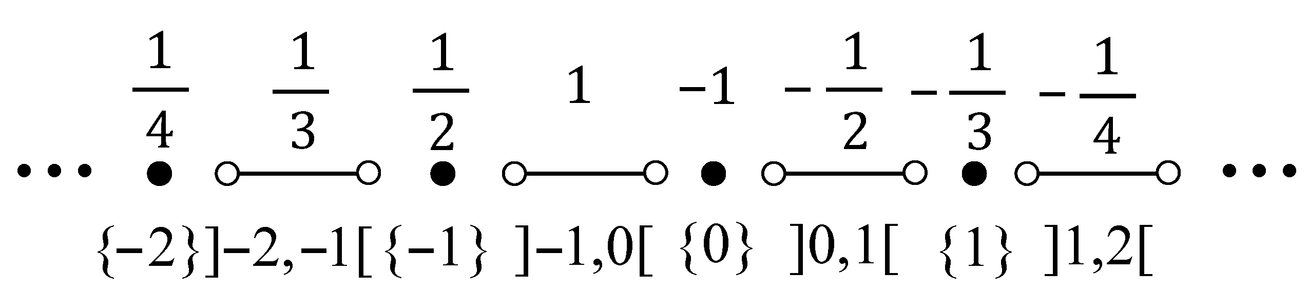
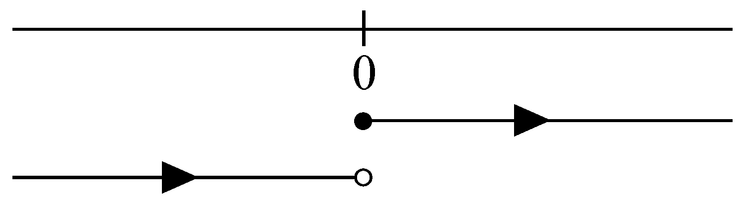
Now, we define the bijection $f:G_1\to Z=\{-\frac{1}{n}:n\in \mathbb{N}\}\cup \{\frac{1}{n}:n\in \mathbb{N}\}$ such that

$$f\left(U_{x1}^{*}\right)=\left\{\begin{array}{ccc}-\frac{1}{2x+1}\hfill & \mathrm{if}& x\in \mathbb{N}\cup \left\{0\right\}\\ -\frac{1}{2(\lfloor x\rfloor +1)}\hfill & \mathrm{if}& x\in [0,\infty [\setminus \mathbb{N}\\ -\frac{1}{2x}\hfill & \mathrm{if}& x\in {\mathbb{Z}}^{-}\\ -\frac{1}{2\lfloor x\rfloor +1}\hfill & \mathrm{if}& x\in ]-\infty ,0[\setminus \mathbb{Z}\end{array}\right.$$

The previous bijection assigns the elements in Z to each $U_{x1}^{*}$, as Figure 1 shows.

Now, if we consider the usual order on Z, it induces an order on $G_1$. Moreover, observe that each $g_i\in G_1$ is decomposed into a finite number of elements in $G_2$. For example, note that $U_{x1}^{*}=U_{x2}^{*}$ for each $x\in \mathbb{Z}$, while $U_{x1}^{*}$ gives us the collection $\left\{\left]\frac{\lfloor x\rfloor }{2},\lfloor x\rfloor +\frac{1}{2}\right[,\left\{\lfloor x\rfloor +\frac{1}{2}\right\},\left]\lfloor x\rfloor +\frac{1}{2},\frac{\lfloor x\rfloor +1}{2}\right[\right\}$ in $G_2$ otherwise. Since that collection is finite, it is discretely ordered with the usual order, and, hence, $G_2$ is ordered with the lexicographic order as explained previously. Therefore, if we list the elements of each $G_n$ according to the order, we have that:

$$G_1=\left\{\left\{0\right\},]0,1[,\left\{1\right\},\dots ,\left\{-1\right\},]-1,0[\right\}$$

$$G_2=\left\{\left\{0\right\},\left]0,\frac{1}{2}\right[,\left\{\frac{1}{2}\right\},\left]\frac{1}{2},1\right[,\left\{1\right\},\dots ,\{-1\},\left]-1,-\frac{1}{2}\right[,\left\{-\frac{1}{2}\right\},\left]-\frac{1}{2},0\right[\right\}$$

$$⋮$$

From that order, we can define a linear order on the completion of the space, $\tilde{\mathbb{R}}$, following Section 3.3, whose topology we denote by ${\tau }_o$. For that, we have to adequately choose the minimum and maximum of each ${\tilde{U}}_{xn}^{*}$. For example, for $]0,1[$, the minimum is the point $\left(\right]0,\frac{1}{2^{n-1}}\left[\right)\in \tilde{\mathbb{R}}$, and the maximum is the point $\left(\right]1-\frac{1}{2^{n-1}},1\left[\right)\in \tilde{\mathbb{R}}$; this is similarly true in the other cases. Note that $0\in U_{0n}^{*}$ and ${\left(\left]-\frac{1}{2^{n-1}},0\right[\right)}_{n\in \mathbb{N}}$ are, respectively, the minimum and the maximum of $\tilde{\mathbb{R}}$.

According to Proposition 17, it follows that ${\tau }_o={\tau }_{{\tilde{d}}^{*}}$ in $\tilde{\mathbb{R}}$. What is more, we can restrict the topology given by the ultrametric in the completion of the original space, and it holds that that restriction gives us the topology of the ultrametric in $\mathbb{R}$. Indeed, it is true due to [5] (Prop. 4.4.10). Figure 2 shows the linear order induced on $\mathbb{R}$ by the order we have defined on $G_n$ for each $n\in \mathbb{N}$.

Note that 0 is the minimum of X with respect to the order and that points which are located on the left of this point in $\mathbb{R}$ are greater than those which are on the right (if we consider the usual order).

In fact, note that since the order is B-compatible, we can forget about the definition of the order on the completion $\tilde{\mathbb{R}}$, since we can define it just from the orders given in each $G_n$, as explained at the beginning of this subsection.

Once we have defined the order according to Herrlich’s construction and the natural fractal structure on $\mathbb{R}$, we consider the cumulative distribution function of a probability measure defined on $\mathbb{R}$ with respect to the usual order. Let us denote that cumulative distribution function by F. Then, the cumulative distribution function given by the new order that we have defined on $\mathbb{R}$ (from the fractal structure), which we can denote by $F_o$, is defined by

$$F_o\left(x\right)=\left\{\begin{array}{ccc}F\left(x\right)-F_{-}\left(0\right)\hfill & \mathrm{if}& 0\le x<\infty \\ F\left(x\right)+1-F_{-}\left(0\right)\hfill & \mathrm{if}& -\infty <x\le 0\end{array}\right.$$

3.5. Defining a Cumulative Distribution Function from a Probability Measure

Now, we study the inverse relationship. If we have defined a probability measure (from a pre-measure satisfying the mass distribution conditions, which can be seen in ([3], Section 3)) on a space with a fractal structure, how can we describe the cumulative distribution function of that probability measure?

Let $\mathsf{\Gamma }$ be a fractal structure on X, and define an order as in the previous subsection. Let $\omega :\mathcal{G}\to [0,1]$ be a pre-measure satisfying the mass distribution conditions such that it induces a probability measure $\mu$ on X, as described in [3,4]. The goal of this subsection is to give a description of the cumulative distribution function of the probability measure $\mu$ in terms of the pre-measure $\omega$.

Given $n\in \mathbb{N}$, let us define $F_n:X\to [0,1]$. Given $x\in X$, then $F_n\left(x\right)$ is defined as $F_n\left(x\right)={\sum }_{y\le x}\omega \left(U_{yn}^{*}\right)$, where the sum is on elements of $G_n$, so $\omega \left(U_{yn}^{*}\right)$ only appears once for each element $U_{yn}^{*}\in G_n$, not for each point $y\in X$.

Finally, $F:X\to [0,1]$ is defined by $F\left(x\right)={\lim }_{n\to \infty }{F}_n\left(x\right)$ for each $x\in X$.

Proposition 19.

F is the cumulative distribution function of the probability measure μ.

Proof. 

Let $F_{\mu }$ be the cumulative distribution function of the probability measure $\mu$. Next, we prove that $F_{\mu }=F$.

Let $x\in X$.

Claim.$(\le x)={\bigcap }_{n\in \mathbb{N}}{\bigcup }_{y\le x}{U}_{yn}^{*}$, where the union is on elements of $G_n$.

It is obvious that $(\le x)\subseteq {\bigcap }_{n\in \mathbb{N}}{\bigcup }_{y\le x}{U}_{yn}^{*}$.

On the other hand, let $z\in {\bigcap }_{n\in \mathbb{N}}{\bigcup }_{y\le x}{U}_{yn}^{*}$. Given $n\in \mathbb{N}$, it follows that $z\in {\bigcup }_{y\le x}{U}_{yn}^{*}$, so there exists $y\le x$ such that $z\in U_{yn}^{*}$. Then $U_{zn}^{*}=U_{yn}^{*}{\le }_n{U}_{xn}^{*}$, and hence $z{\le }_{n}x$. It follows that $z{\le }_{n}x$ for each $n\in \mathbb{N}$ and, hence, $z\le x$, so $z\in (\le x)$. Therefore, the claim is proved.

From the claim and the continuity of the measure from above, it follows that $F_{\mu }\left(x\right)=\mu (\le x)={\lim }_{n\to \infty }\mu \left({\bigcup }_{y\le x}{U}_{yn}^{*}\right)$. Now, given $n\in \mathbb{N}$, note that ${\bigcup }_{y\le x}{U}_{yn}^{*}$ is a union of mutually disjointed sets, and, hence, $\mu \left({\bigcup }_{y\le x}{U}_{yn}^{*}\right)={\sum }_{y\le x}\mu \left(U_{yn}^{*}\right)={\sum }_{y\le x}\omega \left(U_{yn}^{*}\right)=F_n\left(x\right)$.

Therefore, $F_{\mu }\left(x\right)={\lim }_{n\to \infty }\mu \left({\bigcup }_{y\le x}{U}_{yn}^{*}\right)={\lim }_{n\to \infty }{F}_n\left(x\right)=F\left(x\right)$. □

Next, we give an example of the order in Section 3.2.

Example 5.

Let $X={\mathbb{N}}^{\mathbb{N}}$ with the fractal structure given by $\mathsf{\Gamma }=\{{\Gamma }_n:n\in \mathbb{N}\}$, where ${\Gamma }_n=\{\left\{m_1\right\}\times \cdots \times \left\{m_n\right\}\times \mathbb{N}\times \mathbb{N}\times \cdots :(m_1,\dots m_n)\in {\mathbb{N}}^n\}$. Let $x=(x_1,x_2,\dots )\in X$. Then $U_{xn}^{*}=\left\{x_1\right\}\times \cdots \times \left\{x_n\right\}\times \mathbb{N}\times \cdots$ for each $n\in \mathbb{N}$. Note that $d^{*}$ is complete. The order given in Section 3.2 is defined as follows: in $G_n$, define the lexicographic order, that is, $U_{xn}^{*}{\le }_n{U}_{yn}^{*}$ if and only if $x_1<y_1$ or ($x_1=y_1$ and $x_2<y_2$) or …or ($x_1=y_1$, $x_2=y_2$,…$x_{n-1}=y_{n-1}$ and $x_n\le y_n$). Then, the order is defined by $x\le y$ if and only if $x{\le }_{n}y$ for each $n\in \mathbb{N}$.

Consider on X the pre-measure $\omega :\mathcal{G}\to [0,1]$ defined as follows: in $G_1$, the mass is distributed by $\omega \left(U_{x1}^{*}\right)=\frac{1}{2^{x_1}}$ for each $x=(x_1,x_2,\dots )\in X$. Note that the sum of the pre-measure of all the elements of $G_1$ is 1. In $G_2$, given $U_{x1}^{*}\in G_1$, note that $U_{x1}^{*}=\bigcup \{U_{y2}^{*}:y_1=x_1,y_2\in \mathbb{N}\}$. Then we distribute the mass of $U_{x1}^{*}$ (which is $\frac{1}{2^{x_1}}$) in a similar way: $\omega \left(U_{x2}^{*}\right)=\frac{1}{2^{x_1}{2}^{x_2}}$. In general, we can define $\omega \left(U_{xn}^{*}\right)=\frac{1}{2^{x_1}{2}^{x_2}\dots 2^{x_n}}$ for each $x=(x_1,x_2,\dots )\in X$ and each $n\in \mathbb{N}$.

Since $d^{*}$ is complete, then ω defines a probability measure μ on the Borel σ-algebra of $(X,d^{*})$. The cumulative distribution function of μ is given in Proposition 19 as follows.

Given $x=(x_1,x_2,\dots )\in X$, note that $F_1\left(x\right)={\sum }_{i=1}^{x_1}\frac{1}{2^i}=1-\frac{1}{2^{x_1}}$, $F_2\left(x\right)=(1-\frac{1}{2^{x_1-1}})+\frac{1}{2^{x_1}}(1-\frac{1}{2^{x_2}})=1-\frac{1}{2^{x_1}}-\frac{1}{2^{x_1+x_2}}$, and, in general, $F_n\left(x\right)=(1-\frac{1}{2^{x_1-1}})+\frac{1}{2^{x_1}}(1-\frac{1}{2^{x_2-1}})+\cdots +\frac{1}{2^{x_1+\cdots +x_{n-1}}}(1-\frac{1}{2^{x_n}})=1-\frac{1}{2^{x_1}}-\frac{1}{2^{x_1+x_2}}-\cdots -\frac{1}{2^{x_1+x_2+\cdots +x_n}}$.

Then, $F\left(x\right)={\lim }_{n\to \infty }{F}_n\left(x\right)=1-{\sum }_{i=1}^{\infty }\frac{1}{2^{x_1+x_2+\cdots +x_i}}$.

4. Conclusions

This paper serves as a meeting point between the theory on generating probability measures from fractal structures and the one on cumulative distribution functions on separable linearly ordered topological spaces, both developed previously by the authors. First of all, we see how to define a linear order from a space with a fractal structure under a compatibility condition which lets us ensure that the Borel $\sigma$-algebra of the order topology meets the one generated by the topology of the ultrametric induced by the fractal structure. From this connection, we show two examples of linear orders: one that starts from a Polish ultrametric space (note that the completion of a space with a fractal structure is a Polish ultrametric space when working with the ultrametric on the completion and under the assumptions made of the space being $T_0$ and the collection of balls being countable) and another one which is, indeed, a total order with a bottom and a top for which both topologies coincide. Finally, the previous theory and examples let us prove that we can relate the concepts of pre-measure, probability measure and cumulative distribution function as follows. On the one hand, from a cumulative distribution function on a linearly ordered topological space (constructed from a fractal structure), we can define a pre-measure from the collection of balls given by the ultrametric induced by the fractal structure such that its extension is the probability measure whose cumulative distribution function is the original function. On the other hand, given a probability measure on a linearly ordered topological space (which has been constructed from a fractal structure), its cumulative distribution function can be described from a pre-measure defined on the collection of balls given by the ultrametric induced by the fractal structure. This work lets researchers work in the ideal context under their interest when having to treat with these elements of measure theory. Indeed, for authors it is possible to look for applications of both theories by choosing the best context (linearly ordered topological space or fractal structures) in future works.

References

1. Arenas, F.G.; Sánchez-Granero, M.A. A characterization of non-archimedeanly quasimetrizable spaces. Rend. Istit. Mat. Univ. Trieste Suppl. 1999, 30, 21–30. [Google Scholar]
2. Sánchez-Granero, M.A. Fractal structures, in: Asymmetric Topology and its Applications. Quad. Mat. 2012, 26, 211–245. [Google Scholar]
3. Gálvez-Rodríguez, J.F.; Sánchez-Granero, M.A. Generating a probability measure on the completion of a fractal structure. Results Math. 2019, 74, 1–22. [Google Scholar] [CrossRef]
4. Gálvez-Rodríguez, J.F.; Sánchez-Granero, M.A. Generating a probability measure from a fractal structure. Results Math. 2020, 75, 1–28. [Google Scholar] [CrossRef]
5. Gálvez-Rodríguez, J.F.; Sánchez-Granero, M.A. Completion of a fractal structure. Quaest. Math. 2017, 40, 679–695. [Google Scholar] [CrossRef]
6. Li, Z.; Selmi, B. On the multifractal analysis of measures in a probability space. Ill. J. Math. 2021, 65, 687–718. [Google Scholar] [CrossRef]
7. Gálvez-Rodríguez, J.F.; Sánchez-Granero, M.A. The distribution function of a probability measure on a linearly ordered topological space. Mathematics 2019, 7, 864. [Google Scholar] [CrossRef] [Green Version]
8. Gálvez-Rodríguez, J.F.; Sánchez-Granero, M.A. The distribution function of a probability measure on the Dedekind-MacNeille completion. Topol. Appl. 2019, 275, 107010. [Google Scholar] [CrossRef]
9. Gálvez-Rodríguez, J.F.; Sánchez-Granero, M.A. Equivalence between distribution functions and probability measures on a LOTS. Filomat 2021, 35, 4657–4671. [Google Scholar] [CrossRef]
10. Chung, K.L. A Course in Probability Theory; Academic Press: San Diego, CA, USA, 2001. [Google Scholar]
11. Souliotis, G.; Alanazi, Y.; Papadopoulos, B. Construction of Fuzzy Numbers via Cumulative Distribution Function. Mathematics 2022, 10, 3350. [Google Scholar] [CrossRef]
12. Byars, A.; Camrud, E.; Harding, S.N.; McCarty, S.; Sullivan, K.; Weber, E.S. Sampling and interpolation of cumulative distribution functions of Cantor sets in [0, 1]. Demonstr. Math. 2021, 54, 85–109. [Google Scholar] [CrossRef]
13. Roman, S. Lattices and Ordered Sets; Springer: Irvine, CA, USA, 2008. [Google Scholar]
14. Dushnik, D.; Miller, E.W. Partially ordered sets. Amer. J. Math. 1941, 63, 600–610. [Google Scholar] [CrossRef]
15. Bridges, D.S.; Mehta, G.B. Representations of Preferences Orderings; Springer: Berlin/Heidelberg, Germany, 1995. [Google Scholar]
16. Lutzer, D.J. On generalized ordered spaces. Diss. Math. 1971, 89, 42. [Google Scholar]
17. Steen, L.A.; Seedbach, J.A. Counterexamples in Topology; Springer: New York, NY, USA, 1978. [Google Scholar]
18. Schröder, B. Ordered Sets: An Introduction; Springer: Boston, MA, USA, 2003. [Google Scholar]
19. MacNeille, H.M. Partially ordered sets. Trans. Amer. Math. Soc. 1937, 42, 416–460. [Google Scholar] [CrossRef]
20. Edgar, G.A. Measure, Topology, and Fractal Geometry; Springer: New York, NY, USA, 1990. [Google Scholar]
21. Gaba, Y.U.; Künzi, H.-P.A. Splitting metrics by T0-quasi-metrics. Topol. Appl. 2015, 193, 84–96. [Google Scholar] [CrossRef]
22. Engelking, R. General Topology, Revised and Completed Edition, Sigma Series in Pure Mathematics, Volume 6; Heldermann Verlag: Berlin, Germany, 1989. [Google Scholar]
23. Herrlich, H. Ordnungsfähigkeit total-diskontinuierlicher Räume. Math. Ann. 1965, 159, 77–80. [Google Scholar] [CrossRef]
24. Solofomananirina Tiantsoa, F.M. Studies on Ultraquasi-Pseudometrics and Orderings. Master’s Thesis, University of Cape Town, Cape Town, South Africa, 2018. [Google Scholar]
Figure 1. Bijection between G 1 and Z.
Mathematics 10 04518 g001
Figure 2. Linear order induced by the fractal structure Γ in R .
Mathematics 10 04518 g002
Publisher’s Note: MDPI stays neutral with regard to jurisdictional claims in published maps and institutional affiliations.