TALI: An Update-Distribution-Aware Learned Index for Social Media Data

Abstract

In the growing mass of social media data, how to efficiently extract the collection of interested concerns has become a research hotspot. Due to the large size and regularity of social media data, traditional indexing techniques are not applicable. Our “Learned Index”, which is a part of social media intelligence solutions, uses mathematical principles to summarize the laws from the data. It predicts the location of the data by learning the mathematical properties of the data distribution to build the model. Although existing methods over single dimension and multi-dimension such as setting gaps are proposed to further optimize the performance of index, they do not consider the update-distribution of data. In this paper, we propose an update-distribution-aware learned index for social media data (TALI) to support update operations and handle the data sliding. In TALI, underlying data are learned through machine learning models, and a recursive hierarchical model is built. It also learns the update-distribution of data to adjust the size of each leaf node. Thus, it can more effectively support all kinds of operations in databases due to the decrease of the leaf nodes’ sliding. In addition, TALI uses the model-based insertion method for bulkload and query, resulting in a small prediction error. Thus, exponential search is used to perform secondary lookup to improve query efficiency. Experiments were tested and compared on four realistic and synthetic social media datasets. Through extensive experiments, TALI performed better than the existing state-of-the-art learned index with less space occupancy on four realistic and synthetic social media datasets.

1. Introduction

Social Media data come in many forms: Social networking sites, Blogs, Wikis, Reviews, Social bookmarking sites, News portals, and Multimedia sharing websites [1]. The Social Media data extraction and analysis are important as it helps with grabbing the ever-expanding user generated content that companies are interested in for product or service reviews, feedback, complaints, trend watching, and more. It also includes fetching and analysis of specific tweets, followings, likes, updates, group discussions, posts, and so on. Social network community discovery and influence analysis [1], maximal cliques detection and management [2] in social Networks, Knowledge Discovery [3] in Social Networks, and predictive routing scheme [4] for Social Networks are so meaningful that research on social network analysis also flourishes precisely. 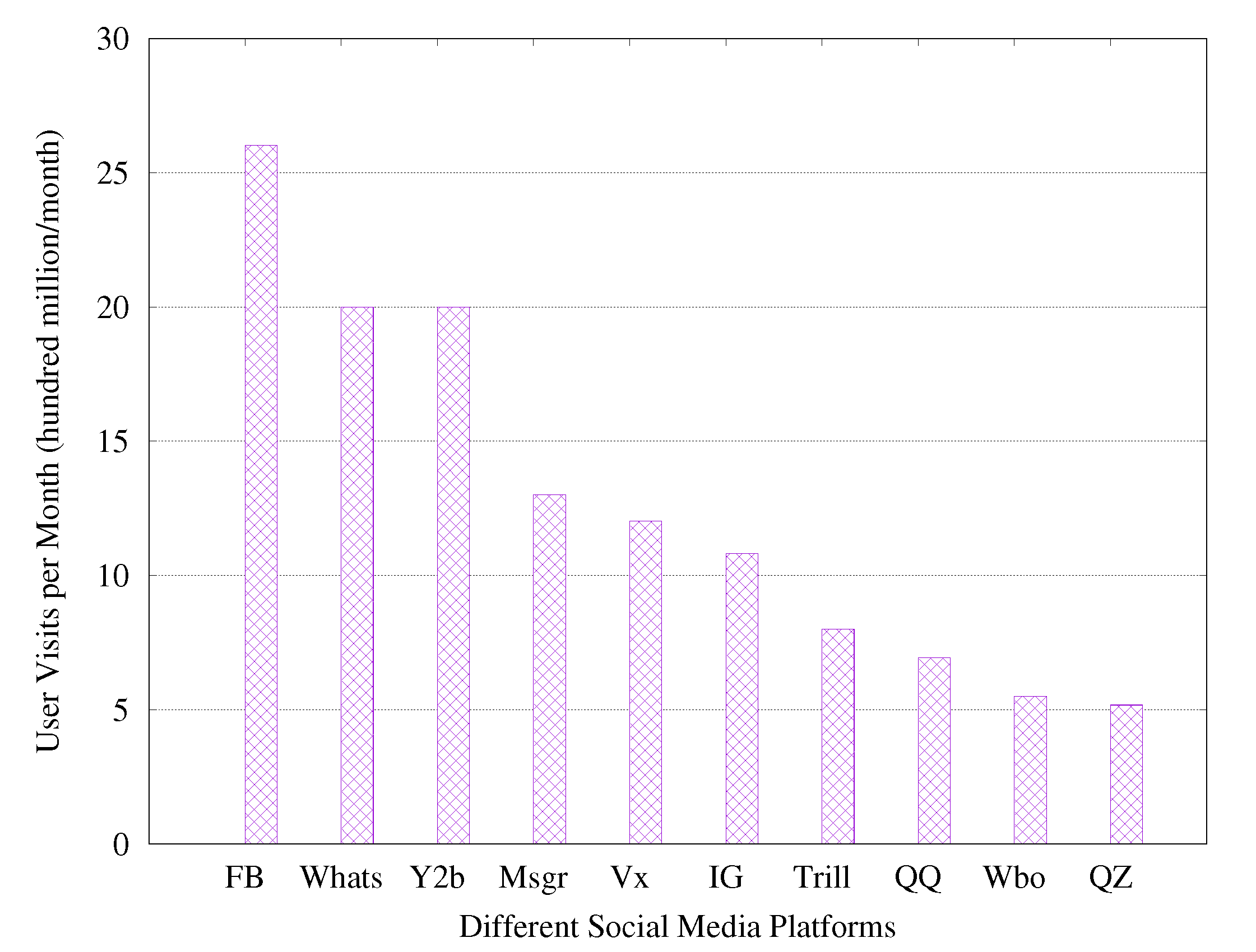As shown in Figure 1, hundreds of millions of users are accessing different social media every moment. In addition, social media data are becoming more and more regular due to the lifestyle of people. For example, people always take the same route to work and always log on to entertainment websites after work. How to use the regularity of social media data to achieve efficient indexing has become a new research problem. Mathematical theories such as linear algebra, probability and statistics, and optimization methods are widely used in the field of AI to express the structure, distribution and update characteristics of data. Therefore, the concept of learned index has been proposed to offer a new direction on indexing with the distribution characteristics of the data. Given a key value, determining the location of the key through the ML model and secondary search is a query operation. An insert operation is given a key to find its corresponding position and insert it into the specified position. For example, in social media databases, a relevant index can be built based on the distribution of user IDs. The user’s login to his account can be regarded as performing a query operation; whenever a new user registers an account, it represents an insert operation to be performed. With the development of social media, it is increasingly difficult for traditional indexes to efficiently process huge social media data. Many studies address the data updates by avoiding the impact of partially contiguous regions (Definition 1, Section 2). However, these learned indexes are limited by the large amount of repeatedly growing data. On the one hand, as a large amount of data are inserted, the distribution of data is becoming increasingly difficult to fit. On the other hand, these learned indexes do not exploit the feature of updating data. For example, users always log in to their accounts after work in the evening.

In this work, to solve the problem of updating social media data, we propose an Update-Distribution-Aware Learned Index for Social Media Data (TALI). To solve the update problem, TALI assumes that the mathematical properties of the data—the update distribution—is known. TALI can change the capacity of nodes according to the data update rule. Other indexes, however, are underutilized the update-distribution to improve performance. TALI dynamically allocates space via learning data and update distribution. Therefore, it could avoid overheads brought by allocating and removing space.

The rest of this paper is organized as follows: Section 2 introduces the background for learned index and related definition. Section 3 expounds the key insight and operations of TALI. Section 4 displays the experiment setup, datasets, and experimental results. Section 5 discusses the related work and results. In addition, finally, we conclude the paper in Section 6.

2. Background and Definition

Index is an indispensable component in the database system. There are rich studies on the traditional index to address different problems. With the development of the ML, a learned index is applied to handling one-dimensional and multi-dimensional problems.

2.1. Traditional Index

Various indexes have been proposed over the last several decades. B-Tree [5] and its variants are fundamental index structures in the modern database system to support database operations. The hash [6] index has been proposed to effectively support point query with hash function. LSM-tree [7] is a hierarchical, ordered, disk-oriented data structure. ART [8] is an adaptive radix tree for efficient indexing in main memory with little storage footprint. Specifically, B+Tree is a dynamic height-balanced tree which is a variant of B-Tree. It provides efficient support for all kinds of index operations. However, all these traditional index structures underutilize the distribution of data to improve the performance of the index.

2.2. Static Learned Index

Many studies advanced new index structures including one-dimensional and multi-dimensional based on ML. RMI [9] first learns the distribution of the data and utilizes CDF to build models to predict the position of keys based on the spline index, which uses spline interpolation to fit data and employs a radix tree and radix table to index data in RS [10]. Pavo [11] proposes a new unsupervised learning strategy to construct the hash function. Flood [12] first proposes a learned multi-dimensional index which chooses optimal layouts and learns query workloads distribution to improve performance. There are two index structures in  [13], which automatically optimize its structure to address data skewed. ZM [14] tunes each partitioning technique to accelerate the index. The ML-index [15] is a multi-dimensional index which partitions the data and proposes a new offset scaling method to transform the point to one-dimensional.

Although these indexes utilize the distribution of data to further improve query performance, all these index structures do not effectively support updatable operations which are necessary in the database and could seriously influence the performance of index.

2.3. Updatable Learned Index

To address the problem of update, [16] uses GA and PMA [17], two layouts to set gaps for inserting to accelerate update performance. In [18], B+Tree leaf nodes are replaced with a piecewise linear model to compress index size. The work [19], which uses a greedy streaming algorithm rather than a greedy algorithm to obtain the optimal piecewise linear model to index data. To achieve real-time update, extra Overflow Array (OFA) is proposed in [20]. The research [21] utilizes a learned index to improve traditional B+Tree performance. XIndex [22] is an index structure which considers the concurrency. Learned index in variable-length string key workloads is effectively achieved in  [23]. The work [24] is a learned index with a previous bloom filter and a post bloom filter. There is a method to eliminate the drift in [25]. LIPP [26] is an index which finishes precise prediction by three item types and the conflict algorithm. The research [27] uses ML models to generate searchable data layout in disk pages for an arbitrary spatial dataset.

Although these index structures support updatable operations, they all underutilize the update-distribution of data. Therefore, in this paper, a new insight is described: learning the update-distribution to lookup and inserting more effectively.

2.4. Related Definition

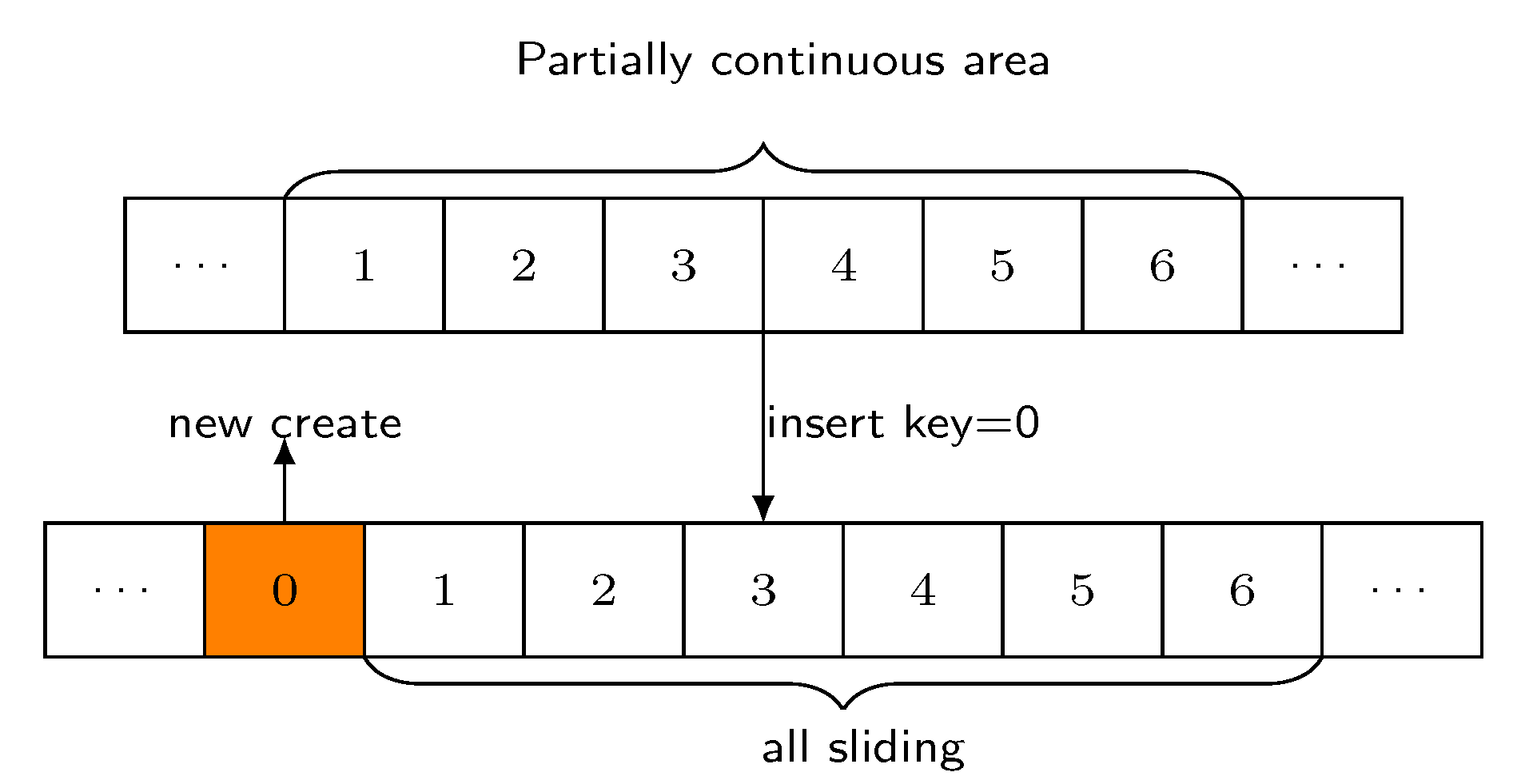
Definition 1. 

Partially continuous area. A partially continuous area is an array of closely linked data. Inserting a key may shift most or even all of these data to finish the operation, as shown in Figure 2.

3. The TALI Index

The TALI takes advantage of two main insights. Firstly, it proposes an approach to accelerate lookup and insert, since inserting a key may cause massive data sliding, which will lead to the actual position being far away from the predicted position in ALEX. The TALI index is presented to reduce the number of sliding by learning the update-distribution of data. Secondly, three hyper-parameters min_num, max_num, and density are defined at each leaf node for better index performance. While maintaining the bound and precision, we go for a smaller number of models. To accomplish robust search and insert performance, an adaptive RMI structure is adopted according to different workloads. The overall design structure of TALI can be seen in Figure 3.

3.1. Overview

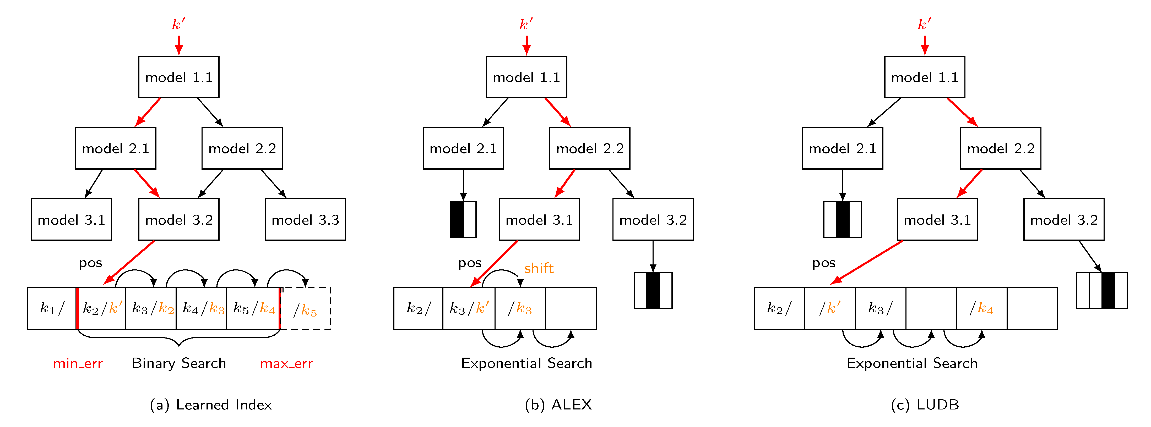
TALI is an in-memory, learning update-distribution, updatable learned index. Compared with a typical B+Tree, TALI stores two or four 8-byte values rather than an array of keys and values in each node. Therefore, TALI has a smaller index size and storage footprint. Furthermore, TALI bases on trained models to predict the position of a key rather than a lot of comparisons and branches. The method can improve search performance because it can directly locate the leaf node of predicted position. While locating the predicted position, TALI uses an exponential search from a predicted position instead of binary search within page size such as B+Tree. If a key needs to be inserted, RMI must create a new array which equals the length of the old array, add one, and shift massive data to create a position. As more keys are inserted, the models will be seriously inaccurate. The cost of insertion will be extremely expensive, and the performance of the insertion will be much lower.

Secondly, TALI adopts a node per leaf like ALEX instead of a single sorted array in a static Learned Index. As is described just now, if a key will be inserted, RMI must create a new array whose length is equal to the old array plus one. Since the array is single without a gap, it must copy all elements to the new array and shift data to make a position (Figure 4a). In the worst case, inserting a key needs to shift all elements. However, TALI adopts a node per leaf with some gaps. Hence, it does not create a new array but only shifts a little data to insert a key (Figure 4c). Therefore, the approach increases insert performance and flexibility as a new element is inserted. In addition, TALI uses model-based insertion to dynamically insert elements. This method utilizes models to predict the position at which the key should be inserted, which improves the insert performance since it decreases the model’s prediction error effectively.

Compared with ALEX, TALI reduces the data sliding by learning update-distribution. Unlike ALEX, which sets gaps only based on initialized data, the bound is broken frequently with more and more elements being inserted. Then, a lot of split and expansion will be implemented and generally shift elements to make an inserted position if a key is inserted (Figure 4b). TALI learns the update-distribution of data to predetermine some gaps for insert keys while bulk loading. It can enhance insert performance because it reduces the split and rewrite time of each node. If a $k_4$ will be inserted after insert $k^{\prime }$ ALEX must expand the node and rewrite keys, TALI can directly insert into its reserved position, as shown in Figure 4b,c. If the model is very accurate, it only needs O(1) to insert. Furthermore, TALI sets a minimum and maximum value to bind the number of each node. It can lessen the number of model nodes to obtain a smaller index size and storage footprint.

3.2. Index Structure

In this section, the two methods LUD and LUDB are introduced. The section also discusses their ideas, implementation process, and related query and update operations.

3.2.1. LUD

To achieve update operations and reduce the data sliding to improve the performance of search and insert keys, TALI first proposes the LUD (Learn Update Distribution) method. It adopts adaptive RMI like ALEX to support insertion effectively, and uses the insight of predetermined gaps to decrease partially continuous areas. As is displayed in Figure 4b, if a conflict occurs on a position which equals 2, ALEX must move nearly all elements to make a gap to finish insertion. This process critically influences the performance of insert operations. Therefore, LUD proposes to reduce the number of nodes splitting, expansion, and predetermined gaps for inserting elements via learning the update-distribution of data. Then, calculate the sum of initial keys and inserting keys. According to the value of allocating corresponding space, this strategy amortizes the cost of shifting data for each insertion. If all the nodes are processed, the merge algorithm will be implemented, based on the merged cost which is less than the cost of nodes and merged in a bottom-up order.

However, the performance of LUD gradually decreases as the inserted data increases. This is due to the fact that, if a node is inserted with a lot of keys, the capacity of the node is too large based on the LUD method. While inserting massive keys in this node, there will be a large number of partially continuous areas which decrease the performance of LUD. Although the performance of LUD gradually decreases, it also achieves slightly higher performance than ALEX as we described in Section 4.

3.2.2. LUDB

To handle the problem of LUD, LUDB (Learn Update Distribution with Bound) is proposed. It also adopts a similar algorithm to LUD. However, when LUDB obtains the number of inserting keys via learning the update-distribution of data and calculates the sum of initial and inserting keys, it does not directly allocate corresponding space according to the sum rather than setting a fixed boundary to limit the capacity of the node. When the sum of initial keys and inserting keys are calculated, LUDB first judges whether the value violates the boundary. If it is violated, the value is too large to allocate space based on the sum, and the capacity of the node equals initial keys divided by initial density. Otherwise, LUDB allocates space based on the sum as described in Section 3.3.

If all the nodes are processed, the merge algorithm will be implemented. This is the second idea of LUDB, which sets the minimum amount of data. To a certain degree, the method can decrease the index size and space occupation. If the count of the node is less than the min_value, the performance of search and insert will not be improved obviously. At the same time, this method can limit the number of models. Therefore, LUDB can spend negligible time cost obtaining a smaller index size. This strategy achieves better index performance to a certain extent.

As for a lookup operation, LUDB first locates the corresponding leaf and then predicts its position based on the model. While finding the predicted position, use an exponential search to locate the actual position of element. It also implements range scan by two point queries. For insert operation, utilize a point query to find the actual insert position first. Then, it judges whether it violates the max_bound or not, if the insert operation violates the boundary of the segment to which the key belongs, moving some other keys to adjacent segments until all segments are violated if inserting a key, implementing an expansion algorithm.

3.3. Bulk Load

To bulk load and build the index, we learn that the CDF is a part of the dataset and build a temporary root model, which outputs a CDF in the range [0, 1] by Equations (1)–(3) to first divide the range of different linear functions based on fixed fanouts. Then, recursively bulk the load based on fanout:

$$a=\frac{1}{max\_key-min\_key}$$

(1)

$$b=-\frac{1}{max\_key-min\_key}\times min\_key$$

(2)

$$y=a\times x+b$$

(3)

where $max\_key$ and $min\_key$ represent the maximum and minimum value of key array, respectively, x represents the input key, and y represents the corresponding position, × represents multiplication, + represents an addition operation, − represents a subtraction operation, and a and b represent sloop and intercept, respectively.

Then, the parameter of each linear function is computed according to Equations (4)–(6), and the number of elements will be inserted:

$$\widehat{{\beta }_1}=\frac{{\sum }_1^n(x_i-\frac{1}{n}{\sum }_1^n{x}_i)(y_i-\frac{1}{n}{\sum }_1^n{y}_i)}{{\sum }_1^n{(x_i-\frac{1}{n}{\sum }_1^n{x}_i)}^2}$$

(4)

$$\widehat{{\beta }_0}=\frac{1}{n}\sum _1^n{y}_i-\widehat{{\beta }_1}\times \frac{1}{n}\sum _1^n{x}_i$$

(5)

$$\widehat{y}=\widehat{{\beta }_0}+\widehat{{\beta }_1}\times x$$

(6)

where $x_i$ and $y_i$ represent each key and the position of the key, respectively; n represents the number of keys and ${\sum }_1^n$ represents sum operation, × represents multiplication, $\widehat{{\beta }_1}$ and $\widehat{{\beta }_0}$ represent sloop and intercept, respectively. x represents the given key and $\widehat{y}$ represents the predicted position. + represents an addition operation, and − represents a subtraction operation.

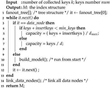
According to CDF, the best fanout tree is built which stores used nodes. Meanwhile, LUDB is based on the cost of each node to decide whether it belongs to a model node or a data node. If the node is a model node, the above process will be executed again. Otherwise, the number of this node and insert keys are calculated. The above process is cyclically executed until each leaf node is small enough. The above procedure is listed in Algorithm 1.

Algorithm 1: Bulkload(k,n).

3.4. Learn Update Distribution

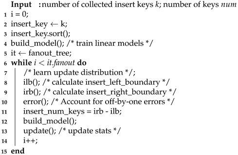
The main insight of this paper is learning the update-distribution of data to reserve gaps in predicted leaf nodes for inserting keys. In Algorithm 2, the Learn Update Distribution algorithm is used as is described to achieve the operation. Firstly, the keys which will be inserted to sort out are collected. Then, use the model and best fanout tree as is described in Section 3.3 to calculate the number of inserting keys in each node. The insert_left_boundary is calculated by Equation (7):

$$ilb=\left\{\begin{array}{cc}0,\hfill & i=0\hfill \\ level[i-1].irb,\hfill & otherwise\hfill \end{array}\right.$$

(7)

where i represents the position of a node in a level of the fanout tree, $ilb$, $irb$ represent the insert_left_boundary and insert_right_boundary, respectively. $level[i-1]$ represents the previous node in this level.

In addition, calculate the insert_right_boundary by Equation (8), and the number of inserting keys equals insert_right_boundary minus insert_left_boundary:

$$irb=\left\{\begin{array}{cc}\left(\right(i+1)-b)/a-k,\hfill & i\ne fanout-1\hfill \\ \left(\right(i+1)-b)/a-k-1,\hfill & i=fanout-1\hfill \end{array}\right.$$

(8)

where $fanout$ represents the number of fanout in this level. a and b represent slope and intercept, respectively, k represents the first key in the insert array, / represents a division operation, + represents an addition operation, and − represents a subtraction operation.

Algorithm 2: TALI(k,n).

While the current node is the first node in this level, the insert_left_boundary equals 0; otherwise, it equals the insert_right_boundary of the previous node. In addition, if the node is the last node in the fanout tree level, the insert_right_boundary equals min between inserting number and calculating the value based on Equation (8). Otherwise, it equals the first value, which is more than the first key of the next node. Note that there may be errors caused by floating-point precision issues, Therefore, LUDB has an extra step to correct the error.

If all data nodes are calculated, then LUDB builds models according to Equations (4)–(6) and allocates space size according to the number of the data node keys and inserting keys as is described in Section 3.3. When the above process is finished, it updates stats at last.

It is important that, if the inserting keys are massive, the overhead that calculates all the elements belonging to each node is expensive. In addition, the entire number of keys and inserting keys in the node are possibly more than the predetermined threshold. To address the problem, LUDB samples a part of the data to estimate the number and set a suitable capacity if there are too many inserting keys. The approach not only decreases the bulk load time but also achieves better index performance.

3.5. Query Operation

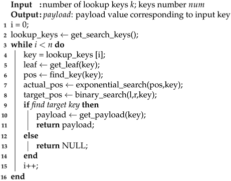
To look up a given key, LUDB starts from the root model of the index structure, and the model is used to compute the leaf node to which the query key belongs. The position of the target key is predicted based on the leaf model. If the given key is located, return its payload; otherwise, return nullptr.

According to the root model the leaf node can be located; then, judge whether the node includes the given key. If the maximum key is less than the given key, the next node of current node will be judged until the given key is found in the range of a node. Otherwise, if the minimum key is also more than the given key, the previous node of the current node will be judged until the correct leaf node is located. Then, predict the position of the given key based on the model of leaf node. If the predicted position is more than the data capacity or less than 0, this represents that the given key is not found. Otherwise, an exponential search will be executed from the predicted position until a key not less than or more than the given key is found. Next, a binary search to locate the first position greater than the key between the position of a given key and the key searched for by exponential search.

Finally, LUDB judges whether the position returned by binary search is the position of the given key. If the key equals the given key, this represents that the given key is found; then, find the corresponding payload of the key and return it. The above procedure is listed in Algorithm 3.

Algorithm 3: Point_Query(k,n).

3.6. Insert Operation

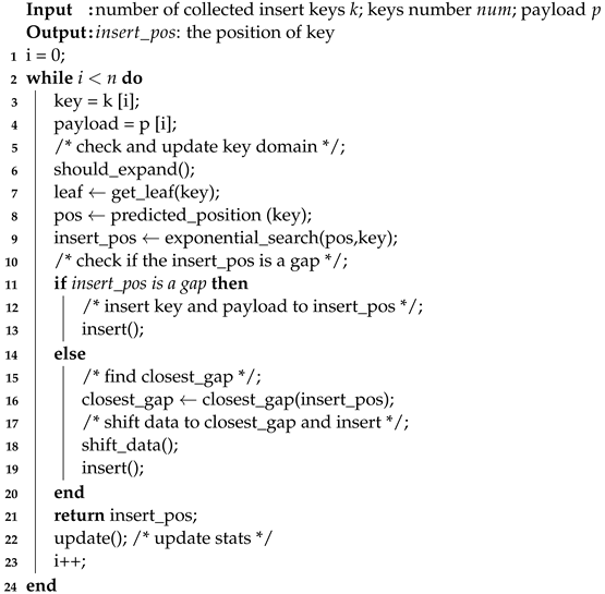
Insert operation is indispensable in database engines to achieve data access dynamically. Inserting a given key, the leaf node is located first according to the root model, and find the target leaf node which includes the given key by comparing the leaf node with its next or previous node. After the target leaf node is found, the position of the given key is predicted by the model of the target leaf node. In addition, then use an exponential search to narrow the range from the predicted position. In the smaller range, use a binary search to locate the precise insert position.

When the precise insert position is located, check whether this insert operation violates the bound of its segment. If this insert does not violate the bound, check whether the inserted position is a gap. If the inserted position is a gap, insert the key to the position directly and update stats. Otherwise, find the closest gap and shift some data to keep a monotonic ascending order. Then, the given key can be inserted into the gap which is created by shifting data.

Otherwise, if inserting a key in this segment violates the bound, shift the maximum key in the current segment to the next segment until no segments will be violated. Then, the given key can be inserted into the inserted position, and the stats are updated. If the boundary of all the segments are violated, expand the node and then rewrite elements and finish the insert operation.

The procedure of inserting the key is described in Algorithm 4. Note that the index may also shift a little data because LUDB does not predetermine inserting gaps in each node due to the capacity bound of each node. However, compared with ALEX, the amount of shifting data is low since LUDB learns the update distribution of data. Therefore, the insert time of LUDB is less than ALEX. Related experimental results will be shown in Section 4.

Algorithm 4: Insert_Operation(k,n,p).

3.7. Other Operations

Delete: Delete operation includes deleting a single key and deleting a range of keys. Deleting a given key LUDB first needs to locate the position of the key by a point query. If the deleted key is found, delete the value and free up the space. Then, judge whether, after deleting a key, the gaps violate the maximum bound. If it violates the bound, we contract the array and copy the data to a new array; otherwise, delete it directly. In addition, delete a range of keys that needs to execute two point queries like range query. Delete from the start key until reaching the position of the end key and updating stats.

Rewrite: If updating the corresponding payload of a key, LUDB first should locate the position of the key by a point query. Then, find the corresponding payload and modify it; stats are updated at last.

Split: If the key cannot be inserted due to massive costs caused by shifting data, then split the current node into two nodes and train its model. Finally, link the data nodes and insert again.

Expand: If the key cannot be inserted due to insertion, a key will violate the maximum bound, expand the node, and copy data to a new array. Then, update the slope and intercept of a new node according to the expand factor.

Contract: If deleting a key violates the maximum value of gaps, LUDB first judges whether a lot of keys will be inserted into the current node. If massive keys are inserted, change the capacity of the node based on the bulk load algorithm described in Algorithm 1. Otherwise, contract and update the slope and intercept of the new node according to the contract factor.

4. Evaluation

In this section, the experiment setup and four datasets used are described. Then, we describe the detailed results such as throughput, index size, average lookup time, average insert time, average sliding per insert, scalability, latency, and lifetime in four workloads. In addition, present the results that compare LUDB with RMI, B+Tree, LIPP, and ALEX in different datasets and workloads. LUDB learns the update distribution of the data to decrease the amount of shifting data and present a merge and contract algorithm to reduce the index size. Therefore, LUDB beats other index structures in different datasets and workloads:

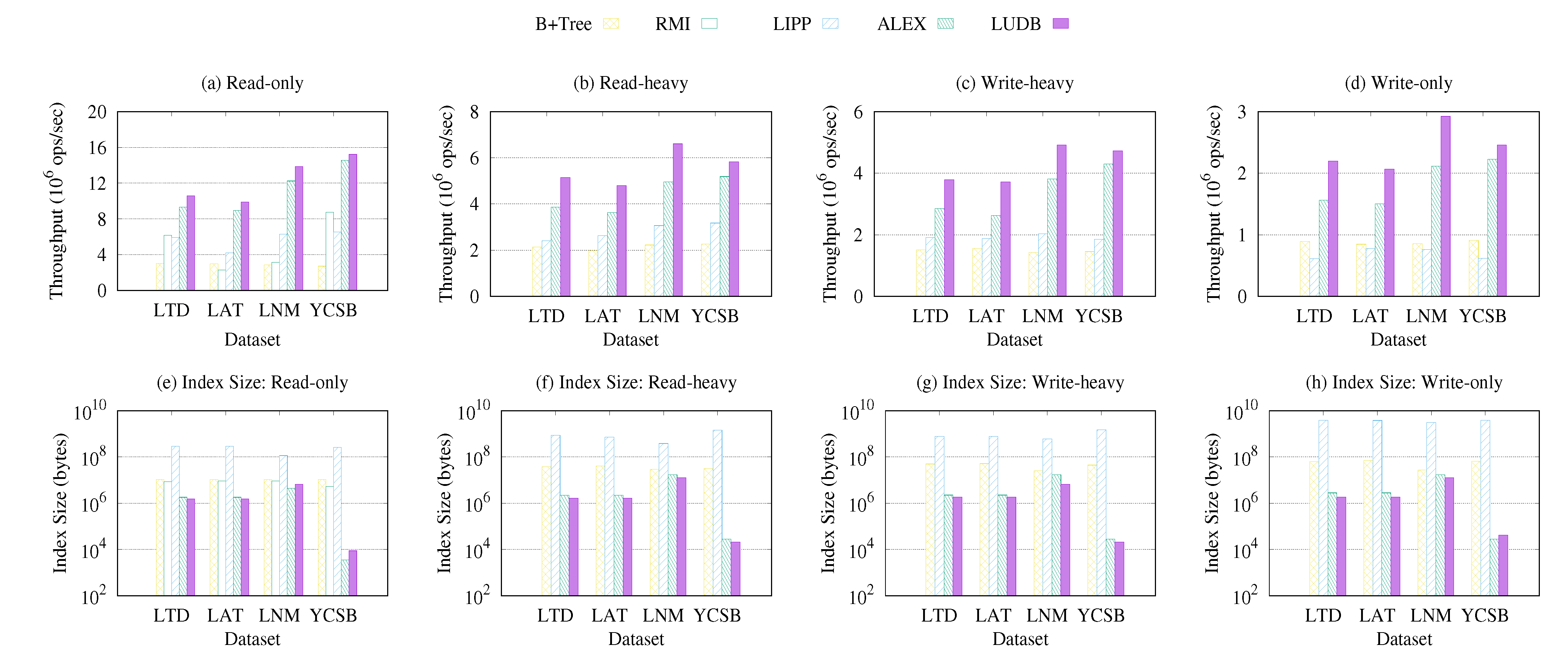
• On read-only workloads, LUDB beats the RMI and LIPP by up to 2.21×, 2.35× search performance and 600×, 30,000× smaller index size, respectively; LUDB also beats the B+Tree by up to 4.65× search performance and 1200× smaller index size; but LUDB achieves only comparable performance and index size with ALEX;
• On read-only workloads, LUDB beats the RMI and LIPP by up to 2.21×, 2.35× search performance and 600×, 30,000× smaller index size, respectively; LUDB also beats the B+Tree by up to 4.65× search performance and 1200× smaller index size; but LUDB achieves only comparable performance and index size with ALEX;
• On write-heavy workloads, LUDB achieves up to 1.42× operation performance and 2.59× smaller index size than the ALEX; and beats the B+Tree by up to 3.58× performance and 2100× smaller index size. LUDB also achieves 2.45× higher performance and 72,000× smaller index size than LIPP;
• On write-only workloads, LUDB beats the B+Tree by up to 3.40× operation performance and 1500× smaller index size; and beats the ALEX by up to 1.42× operation performance and comparable index size. LUDB also achieves 3.84× higher performance and 93,000× smaller index size than LIPP.

4.1. Experiment Setup

In this part, the environment, datasets, workloads, and baselines of the experiment are described in detail.

4.1.1. Environment

LUDB is implemented in C++ and compiled with GCC 9.4.0 in O3 optimization mode. All of the experiments are conducted on an Ubuntu 20.04 Linux machine9 (Canonical, London, UK) with 2.8 GHz Intel Core i7 (2 cores and 2 threads) and 8 GB memory.

4.1.2. Datasets

LUDB uses a key-payload pair to accomplish index operations, where key is an 8-byte value from the dataset, and payload is a randomly generated fixed-size value. The experiments are run using four popular social media benchmarks (path information and user ID information) listed in

Table 1. Datasets.

Parameter	LTD	LAT	LNM	YCSB
Num keys	1B	200 M	190 M	200 M
Key type	double	double	int64	int64
Payload size	8 B	8 B	8 B	80 B
Total size	16 GB	3.2 GB	3.04 GB	17.6 GB
bulkload keys	1 × ${10}^7$	1 × ${10}^7$	1 × ${10}^7$	1 × ${10}^7$
Total num	1 × ${10}^8$	1 × ${10}^8$	1 × ${10}^8$	1 × ${10}^8$

to evaluate the method.

• LTD: The LTD dataset consists of the longitudes of locations around the world from Open Street Maps [28];
• LAT: The LAT dataset consists of compound keys which combine the longitudes and latitudes from Open Street Maps by applying the transformation to each pair of longitudes and latitudes. The distribution of the longlat dataset is highly nonlinear;
• LNM: The LNM dataset is generated artificially according to a lognormal distribution;
• YCSB: The YCSB dataset is also generated artificially, which represents the user IDs according to the YCSB Benchmark. The dataset follows the uniform distribution and uses an 8-byte payload.

Unless stated, the above datasets do not contain duplicated elements. We simulate the real-world scenarios by randomly shuffling these four datasets.

4.1.3. Workloads

Average throughput is the primary metric to evaluate the performance of LUDB compared with other different index structures. To suggest the performance of different operations, the throughput, index size, average lookup, and insert time are evaluated on four different workloads:

• The read-only workload, which only performs lookup operations on the indexes;
• The read-heavy workload, which contains 30% writes to insert the element into indexes and 70% reads to lookup keys;
• The read-heavy workload, which contains 50% writes to insert the element into indexes and 50% reads to lookup keys;
• The write-only workload, which only contains write operations to insert keys.

For all four of the workloads, read operation represents looking up a single key, which is selected randomly from the set of existing keys in the index according to a Zipfian or a uniform distribution. Therefore, a lookup operation will always locate the key. Given a dataset, the indexes are first built and bulk load is according to Table 1. Then, running a given workload for 60 s and report the total number of operations completed in that time. These operations are either inserts or lookups. Specifically, for the read-heavy workload, it performs 7 reads, then 3 insertions, then repeats the cycle; for the write-heavy workload, it performs 1 read, then 1 insertion, then repeats the cycle; for the write-only workload, we only perform insert operations on the indexes.

4.1.4. Baselines

The LUDB is compared with four existing index structures:

• Standard B+Tree: it is implemented as STX B+Tree. The STX B+ Tree is a set of C++ template classes implementing a B+ tree key/data container in main memory. It can achieve all kinds of index operations;
• RMI: it is a static index structure which uses two levels RMI to lookup;
• LIPP: it is a precise index structure to finish lookup and insert, which uses three-item types to address the problem of “last mile”;
• ALEX: which is an updatable adaptive learned index in memory. It uses gaps to achieve insert operation and a flexible layout to improve performance.

To evaluate these index structures’ throughput, index size and average lookup and insert time as main parameters are calculated. To measure throughput for LUDB, ALEX, B+Tree, and RMI, all of these indexes first calculate the throughput of each batch, then obtains the overall throughput. To measure index size for B+Tree, one only needs to calculate the sum of all inner node sizes. For RMI, ALEX, and LUDB, they calculate the sum of all model node sizes, which include pointers and metadata. To measure average lookup and insert time, lookup and insert throughput of each batch are calculated first; then, calculate average lookup and insert time of each lookup or insert operation according to throughput.

4.2. Result Analysis

In this section, the experimental results are analyzed in four different datasets. The results suggest that the performance of LUDB gradually decreases as the insertion ratio increases, but performance gradually becomes higher than ALEX, LIPP, and B+Tree. This is because insert operations are more time-consuming than lookup operations. Furthermore, since LUDB learns the update-distribution of the data as described above, LUDB always has higher performance as the insertion ratio increases. Due to the fact that LUDB uses bounds to limit the capacity of nodes, the index size of LUDB is always less than ALEX and B+Tree.

4.2.1. Read-Only Workloads

For read-only workloads, LUDB achieves up to 4.65×, 2.35×, and 2.21× throughput compared to B+Tree, LIPP, and RMI, as shown in Figure 5a. Compared with B+Tree and RMI, LUDB adopts a gaps array and flexible node layout like ALEX; it sets a bound to decrease the influence of a partially continuous area. It also utilizes segments to support the index effectively. Furthermore, the error between the predicted position and actual position is small because LUDB uses a based-model method to insert. LUDB uses an exponential search instead of a binary search within an error bound. For each lookup, the search method needs to find the actual position according to the predicted position. Because the error is small, exponential search can be faster for locating the actual position. However, B+Tree and RMI do not use a based-model method for insertion so the error is bigger than LUDB. In addition, they use binary search in error bound, so the search performance is lower. LIPP is a precise index to support query and insert, but as the number of keys increases, it needs massive time and space to maintain the index. We use ${10}^7$ to bulk load and based on the structure to query, as shown in Figure 5a. LIPP only has a similar performance to RMI and one that is worse than LUDB. The LAT data distribution is highly nonlinear so it is more difficult to model. Therefore, LUDB has lower throughput compared with other datasets.

LUDB also achieves up to five orders of magnitude, 600×, 1200× index size smaller than LIPP, RMI, and B+Tree, as shown in Figure 5e. The index size of LUDB depends on how well the index structure models the dataset distribution. For the YCSB dataset, it is highly linear, so LUDB does not need massive models to model the distribution. Then, the index size of the dataset is smaller than other datasets. However, for the LAT dataset, which is highly nonlinear, LUDB requires many models to model its distribution, so it has a larger index size compared with other datasets. This phenomenon suggests that, if LUDB only needs a few models, it will have higher throughput and smaller index size. Furthermore, LUDB also sets a bound of node sizes to achieve faster merge operation and smaller index size. Then, LUDB can reduce bulk load time and obtain a better index performance.

However, since there is no insert operation, we cannot learn the update-distribution. Therefore, LUDB is only the same as ALEX on search performance and index size, as shown in Figure 5a,e.

4.2.2. Read-Write Workloads

Figure 5b,c and Figure 6 show that LUDB achieves up to 3.58× higher performance than the B+Tree and up to 1.42× and 2.45× higher perfermance than ALEX and LIPP. Since the RMI cannot effectively support update operations, we do not include it in read-write and write-only workloads. The results show that the LUDB, which beats other index structures on three datasets, expects to be comparable with ALEX for the YCSB dataset. Because YCSB has uniform distribution, LUDB sets a merge bound to accelerate merge and decrease index size. However, YCSB only needs 20 models to model it by ALEX, but LUDB needs 30 models to model it according to the merge bound. Obviously, this method decreases the throughput on performance if the dataset has uniform distribution.

Conversely, this method is well used in the other three datasets, as shown in Figure 5b. Because the three datasets are not as easy to model as YCSB, especially the LAT dataset, which is highly nonlinear, it is not easy to model its distribution so it will lead to massive expansion and split operations. Then, a lot of data sliding will happen and lead to the predicted position of a given key being far from its actual position. However, LUDB learns the update-distribution of data, so it can pre-allocate positions for inserting keys. This method avoids lots of data sliding to improve performance.

Figure 5f,g and Figure 6a,b suggest that LUDB beats B+Tree, LIPP, and ALEX by up to 2100×, 72,000×, and 2.59× smaller index size. For B+Tree, since it does not have any obvious tunable parameters other than page size, it only changes page size to obtain better performance and smaller index size. If looking up or inserting a key, there are massive launches and comparisons to locate the leaf node of the given key. Then, it has a binary search on page size. However, LUDB only consists of two double-precision floating point numbers in each model, which represent the sloop and intercept of a linear regression model. Therefore, the size of a model node in LUDB is less than one of an inner node in B+Tree. For ALEX, similar to throughput on performance, the index size is based on how well the models model its distribution. For LIPP, in order to maintain the precise position, it needs extra space to store the item types. With the number of insert keys increasing, the index size of LIPP will increase accordingly.

4.2.3. Write-Only Workloads

Figure 5d shows that LUDB also achieves better performance than B+Tree, LIPP, and ALEX, and it achieves up to 3.40× higher throughput than the B+Tree, up to 3.84× higher throughput than the LIPP, and up to 1.42× higher throughput than ALEX. The LUDB still beats ALEX on three datasets and has comparable throughput on YCSB.

Figure 5h displays the index size on write-only workloads. In general, the index size of LUDB and ALEX will be bigger with the number of insert keys increasing. Since the B+Tree is robust, it may slightly increase with the number increasing. Due to LIPP needing space to store the item types, as the number of insert keys increases, the index size of it also will be higher.

4.3. Detailed Performance Study

In this section, the scalability, data sliding, and latency of LUDB, ALEX, LIPP, and B+Tree on four different datasets and four different workloads are discussed.

4.3.1. Scalability

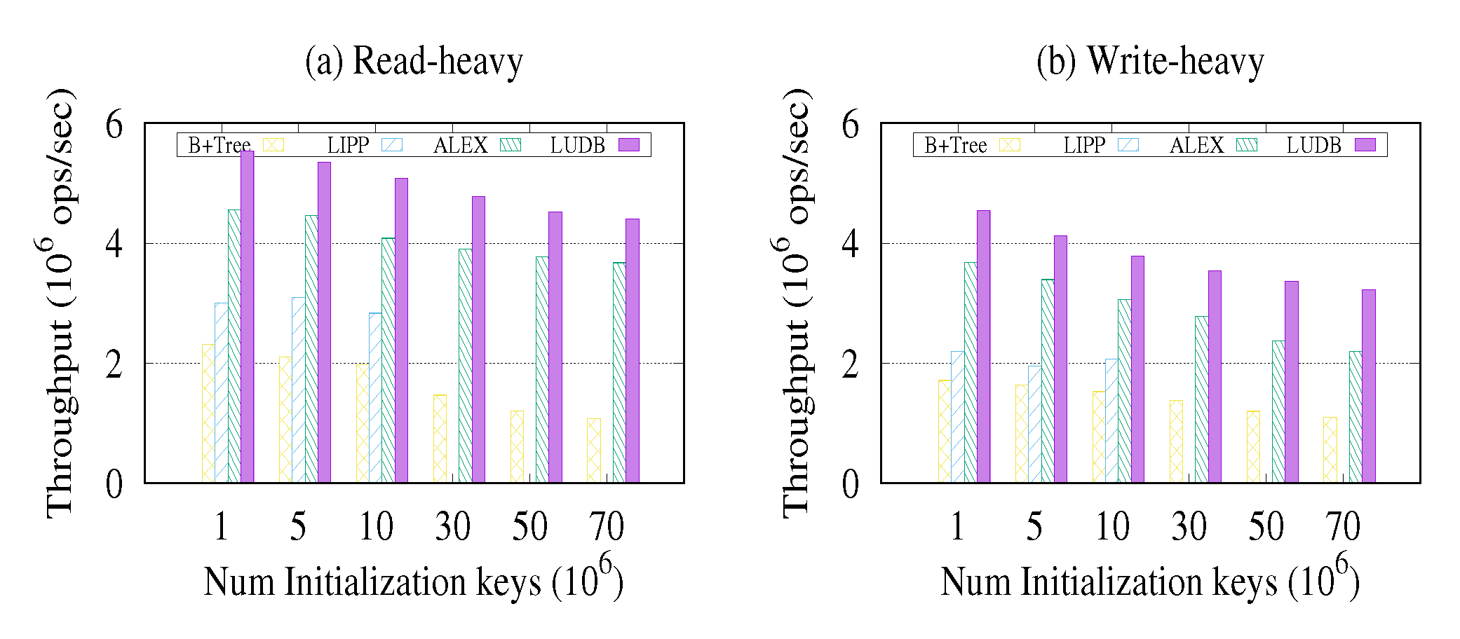
To explore the scalability of the LUDB, the LTD dataset is run on read-heavy and write-heavy workloads as shown in Figure 7. The total number of keys equals ${10}^8$ and batch size equals ${10}^6$. Then, change the number of initialization keys instead of a fixed number and record its corresponding throughput. As the number of initialization keys increases, LIPP cannot support index operation, as shown in Figure 7. This is because the index size and data size are too big to support index operations as discussed before. Figure 7 demonstrates that, although the overall performance decreases as the number of initialization keys increase, LUDB still maintains a better performance than ALEX and B+Tree on read-heavy and write-heavy workloads. Furthermore, due to the fact that LUDB maintains a fixed bound and density for keys and learns the update-distribution of data, the rate of throughput decreases slowly. In addition, it has gaps for keys, so for inserting a key, the time does not increase a lot. Therefore, LUDB performance can scale well to larger datasets.

4.3.2. Latency

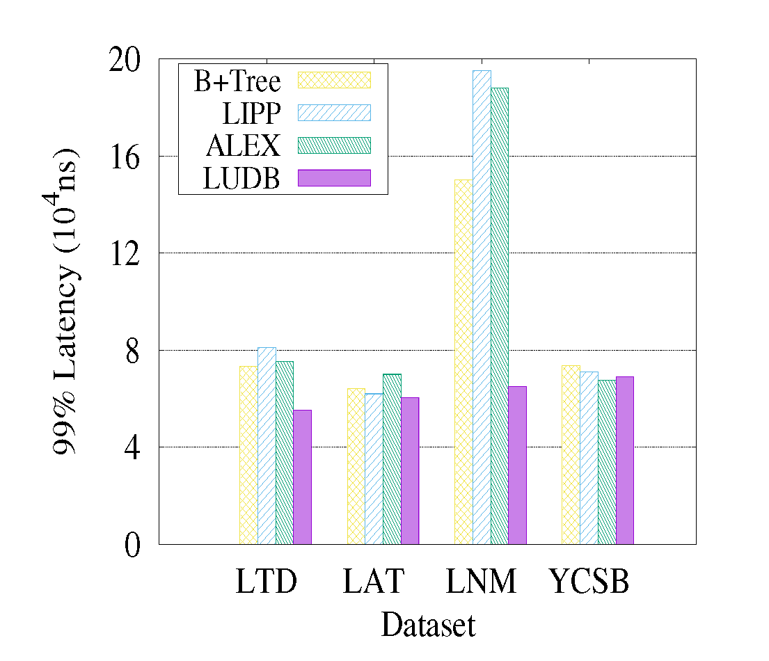
To further display the inner performance of LUDB compared with other index structures, this paper compares LUDB with B+Tree, LIPP, and ALEX on write-only workloads and uses 1000 keys to calculate the latency of insert. Figure 8 demonstrates the 99th percentile latency while implementing insert keys until reaching 1000. Each batch size is 100. The 99th percentile latency of LUDB on LTD and LAT datasets beats ALEX, LIPP, and B+Tree by up to 1.33×, 1.47×, and 1.36× lower time. In particular, LUDB has a smaller 99th percentile latency on the LNM dataset, but ALEX has a larger 99th percentile latency. This is because the distribution of the first one thousand keys in the LNM dataset is not uniform, and ALEX needs a large number of shift operations to insert a key, which causes higher latency. However, due to the fact that LUDB learns the update-distribution of inserting data, it can address the problem of massive sliding and has smaller insert latency. However, on the YCSB dataset, LUDB has a higher 99th percentile latency than ALEX and B+Tree. Since B+Tree can deal with datasets which have different distributions, the performance of B+Tree is therefore neither good nor bad; however, the distribution of the dataset is uniform or highly nonlinear. In addition, due to the fact that the distribution of YCSB is uniform, ALEX can model it by only a few models. Then, it has a better performance and a smaller 99th percentile latency. Although LUDB learns the distribution of data, it also sets a merge bound and a density bound, which causes more models to model its distribution. Therefore, it has poor performance and a higher 99th percentile latency. However, as Figure 5 and Figure 6 displayed, the performance of LUDB is better as the insert number is increasing. In addition, in the real world, the dataset is enormous, so it will have comparable performance with ALEX on LAT.

4.3.3. Data Sliding

As shown in Figure 9, LUDB beats ALEX by up to 3.8× lower data sliding on all datasets. Specifically, on the LAT dataset, whose distribution is highly nonlinear, LUDB also achieves 3.1× lower average sliding per insert than ALEX. This is why LUDB can accomplish better performance compared with ALEX on this dataset. Furthermore, the number of average data sliding per insert decreases as the insert fraction increases.

Because LUDB and ALEX both set a maximum segment bound and node density, inserting massive keys will violate the bound of the node. Then, it will expand or split the node and reallocate the keys based on a fixed gap. After reallocating the predicted position of an insert key to be very close to its actual position, the average sliding per insert decreases correspondingly.

Figure 9 also shows that LUDB is only slightly decreased compared with ALEX on the YCSB dataset. As described in the above sections, the merge bound method increases the number of models to model its distribution due to the fact that the YCSB has uniform distribution. Therefore, it may lead to slightly lower performance than ALEX, but as the number of models increases, each model has a smaller length than less models, which causes lower average sliding. This is why LUDB has lower performance than ALEX but has lower average sliding per insert.

4.3.4. Lifetime Study

LUDB has a better lifetime than ALEX, LIPP, and B+Tree. Figure 10 displays average lookup time and average insert time on LTD and LAT datasets. The total number of keys equals ${10}^8$, the number of initial data equals ${10}^6$, and each batch size equals ${10}^6$. Then, change the insert proportion and calculate different index structures, which correspond with the average lookup time and average insert time.

Figure 10 suggests that, even with increasing the number of insert keys, LUDB still has lower average lookup and insert time. Figure 10a indicates that, on the LTD dataset, LUDB has an average lookup time similar to ALEX, but achieves up to 5.31×, 3.10× shorter than B+Tree and LIPP because ALEX also uses a model-based method to insert and LTD is not highly nonlinear. ALEX and LUDB both use adaptive RMI; it does not grow over time and gaps are maintained according to the density. However, B+Tree and LIPP must have a series of split and re-balance operations while inserting a large number of keys. Therefore, B+Tree and LIPP grow deeper over time, which makes lookup costs expensive. For inserts, LUDB has 1.32× lower average insert time than ALEX, 2.07× lower than B+Tree, and 1.93× lower average insert time than LIPP, as shown in Figure 10b. Because ALEX does not learn update-distribution for inserting keys, its array still contains partially continuous areas which will reduce the performance of ALEX.

Figure 10c,d shows that, even on the LAT dataset, which is highly nonlinear, LUDB also beats ALEX by having a slightly lower average lookup time and achieves a much lower average insert time than ALEX, LIPP, and B+Tree. Although LUDB learns the update-distribution of data, the LAT dataset is highly nonlinear, so it does not model it perfectly either. Therefore, the performance of LUDB on the LAT dataset is degraded compared to other datasets. All these phenomena suggest that LUDB has a long lifetime and better performance than the other three indexes.

5. Discussion

In this section, relevant experiments and results are discussed.

B+Tree: B+Tree uses split and merge operations to finish the update operations. By packing multiple value pairs into each node of the tree, the B+tree reduces heap fragmentation and utilizes cache-line effects better than the standard red-black binary tree.

RMI: RMI uses the Cumulative Distribution Function (CDF) of the dataset to train models and build the Recursive Model Index. Then, it learns the distribution of data to build models that predict the position of a key in the database. Due to the existing errors of the ML models, the position predicted by the model may be not accurate. RMI needs to have a binary search between min_error and max_error to locate the accurate position. However, because RMI stores data in a tight array, it cannot handle data updates efficiently.

ALEX: It is a learned index which can effectively handle data updates and use an adaptive RMI structure to handle different data distributions. ALEX utilizes two leaf node layouts gap array (GA), and packed memory array (PMA) to process updates. When inserting a key, a point query will be executed to find the position of the key. If the current position is the reserved gap, it can be directly inserted; otherwise, the insertion is done by moving the data to create a gap. In addition, ALEX uses exponential search instead of binary search because ALEX uses model-based insertion to make it easier for the lookup to fall near the correct position. However, ALEX has to move a lot of data to process updates when the data are updated frequently, and this can cause a dramatic drop in performance.

LIPP: It implements precise queries by building a tree-structured learned index to handle data conflicts. It solves data conflicts through three types of items, and uses the FMCD algorithm to calculate the conflict degree and then trains the model according to the conflict degree. LIPP also designs a merge strategy to control the height of the tree and reduce space overhead. However, LIPP is still limited by large data volumes because it stores real data at nodes, and performance is affected by tree height.

TALI: To achieve update operations and reduce the data sliding to improve the performance of search and insert keys, TALI first proposes to first reduce the number of node splitting, expansion, and predetermined gaps for inserting elements via learning the update-distribution of data. It adopts adaptive RMI like ALEX to support insert effectively, and uses the insight of predetermined gaps to decrease partially continuous areas. It also sets the boundary of data capacity to improve performance and the minimum amount of data to limit the number of models. Therefore, compared with other index structures, TALI can achieve better index performance.

Since TALI learns to the update distribution of the data, it can better handle the update data sliding situation. At the same time, the impact of partial continuous regions on index performance is reduced, so it can be well scaled to large datasets.

6. Conclusions

In this paper, an index structure TALI is proposed which learns the update-distribution of social media data to solve the problem of frequent and regular updates of social media data. TALI efficiently solves the indexing problem of frequently updated social media data, and improves the performance of querying and inserting social media data by learning the basis of social media data and update distribution law. This approach results in better overall performance and improves the performance of query and insertion. Since TALI adopts adaptive RMI and gaps like ALEX, it can address datasets with different distributions and workloads. Because TALI is less affected by partial continuous regions, it can be well extended to large data sets and has a certain robustness. Experimental results suggest that TALI beats B+Tree, LIPP, and RMI on four datasets and workloads, and beats ALEX on three of the four datasets. Specifically, there are no insert operations on read-only workloads, so TALI has a similar performance to ALEX.