Article

A New Fractal-Fractional Version of Giving up Smoking Model: Application of Lagrangian Piece-Wise Interpolation along with Asymptotical Stability

1
Department of Mathematics, Azarbaijan Shahid Madani University, Tabriz 3751-71379, Iran
2
Engineering Mathematics, School of Engineering, University of Namibia, Windhoek 13301, Namibia
3
Department of Mathematical Sciences, Federal University of Technology, Akure PMB 704, Nigeria
4
Laboratory of Applied Mathematics, Kasdi Merbah University, Ouargla 30000, Algeria
5
Department of Computer Engineering, Faculty of Engineering, Final International University, via Mersin 10, Kyrenia 99300, Northern Cyprus, Turkey
6
Department of Medical Research, China Medical University Hospital, China Medical University, Taichung 40402, Taiwan
7
Department of Mathematics, Texas A&M University-Kingsville, Kingsville, TX 78363, USA
*
Authors to whom correspondence should be addressed.
Mathematics 2022, 10(22), 4369; https://doi.org/10.3390/math10224369
Submission received: 22 September 2022 / Revised: 10 November 2022 / Accepted: 15 November 2022 / Published: 20 November 2022
(This article belongs to the Special Issue Recent Advances in Theory and Application of Dynamical Systems)

Abstract

:
In this paper, a new kind of mathematical modeling is studied by providing a five-compartmental system of differential equations with respect to new hybrid generalized fractal-fractional derivatives. For the first time, we design a model of giving up smoking to analyze its dynamical behaviors by considering two parameters of such generalized operators; i.e., fractal dimension and fractional order. We apply a special sub-category of increasing functions to investigate the existence of solutions. Uniqueness property is derived by a standard method based on the Lipschitz rule. After proving stability property, the equilibrium points are obtained and asymptotically stable solutions are studied. Finally, we illustrate all analytical results and findings via numerical algorithms and graphs obtained by Lagrangian piece-wise interpolation, and discuss all behaviors of the relevant solutions in the fractal-fractional system.

1. Introduction

Smoking has always been one of the known causes of many human diseases, which threatens the physical health of a large part of the world’s population (both smokers and non-smokers). The impact of tobacco abuse, especially cigarettes, on different parts of the human body can be seen so clearly that one of its primary effects is the death of more than 5,000,000 people per year. If we want to make a comparison between smokers and non-smokers, we can refer to the results of medical reports in hospitals around the world, in which the rate of heart attacks and the prevalence of lung cancer in smokers compared to non-smokers are more than 70% and 10%, respectively. Even based on the reports of WHO, the lifespan of non-smokers has been reported to be 10 to 13 years longer than that of smokers. Smoking in the short term can cause bad breath, yellowing of teeth, wrinkled skin, persistent cough, and high blood pressure. In the long term, this bad habit causes dangerous diseases such as stomach ulcers, heart diseases and cancers such as lung, mouth and gums, and throat.
Due to the widespread use of tobacco among teenagers and even children, every year the World Health Organization requests researchers and doctors to study its effects on people’s health and present the results in the form of detailed reports and charts and tables. Recently, using the data and numerical results of such studies, researchers have done mathematical modeling of the process of smoking in various statistical societies, and using mathematical algorithms and computer calculations, they are trying to provide methods to control and optimize the outputs. In this direction, researchers turned to mathematical tools and models, and tried to simulate the dynamics of processes and phenomena with the help of differential equations (ordinary and partial) and to get accurate solutions by solving them. Zaman [1] in 2011 designed a model of giving up smoking and analyzed the system qualitatively. In 2008, Sharomi et al. [2] proposed a system of curtailing smoking in the form of four differential equations and investigated stable and unstable solutions. After that, Alkhudhari et al. [3] suggested a four-compartmental system of smoking and checked the effect of smokers on temporary quitters based on the equlibrium criteria. Rahman et al. [4] studied an age-structured model of giving up smoking and conducted an optimal analysis. In addition, in another work, Rahman et al. [5] extended their model of giving up smoking by considering the harmonic mean incidence rate. Other full studies can be found in this regard such as Refs. [6,7].
Due to the weakness of classical operators, generalized fractional operators (Caputo–Fabrizio [8] and Atangana–Baleanu [9]) quickly attracted the attention of many researchers. The non-locality property of the new operators along with their memory property narrowed the field to classical operators such as Riemann–Liouville and Caputo [10]. Of course, there were still those who used classical operators for their modeling to study the dynamics of smoking. For instances, Erturk et al. [11] constructed a five-compartmental fractional giving up smoking model (based on the standard model [12]) via the singular Caputo derivative, and by using the MSGDT method, derived the approximate solutions and lastly, compared their results with the data obtained by the Runge–Kutta algorithm. Zeb et al. [13] gave another fractional model of such a phenomena and analyzed it via the HAM technique. Finally, the giving up smoking and smoking cessation models have been evaluated with various parameters and control tools in different mathematical models with new nonsingular operators, among which we can refer to the research articles published in Refs. [14,15,16].
More recently, another class of hybrid two-parametric operators was given by Atangaga, for which we can derive more accurate numerical outputs in comparison to both fractional and integer-order operators [17,18]. Due to the effect of fractal dimension and fractional order in the final result, these operators are called “Fractal-Fractional Operators". In the structure of these operators, the role of fractal derivative is essential, and by considering the kernels, these operators divide into three types called the Power law, exponential decay law, and generalized Mittag–Leffler law-type fractal-fractional operators. For more information, one can refer to [17,18]. The effectiveness and efficiency of new operators in obtaining accurate results can be seen in a large number of relevant studies [19,20,21,22,23,24,25,26,27,28,29].
To state the contribution of our work, as we said above, we know that the classical standard time-derivatives are local operators and have some weaknesses in the prediction of the dynamics of a phenomenon. Even a well-known fractional derivative such as the Caputo–Liouville has its own limitations. Since its kernel has a weak memory effect in comparison to the newly-defined fractal-fractional derivatives, this type of derivative cannot precisely describe the full effect of the memory. Hence, due to the strong memory effect, complex dynamics, and non-locality of the generalized hybrid fractal-fractional operators, our main objective in the present research is to use the novel two-parametric power-law type ( ϰ 1 , ϰ 2 ) -fractal-fractional derivative to model the giving up smoking efficiently. In addition, dynamics of the supposed fractal-fractional model is predicted by a numerical scheme with respect to two fractional and fractal parameters continuously for which we can analyze some behaviors of the system accurately.
The rest of the paper is organized as follows. Section 2 deals with preliminaries and Section 3 describes the extended model. Mathematical analysis is carried out in Section 4, whereas in Section 6, the numerical simulations are done based on the algorithms derived in Section 5. Section 7 concludes the paper.

2. Preliminaries

In this section, we recall some basic definitions and theorems about fixed point theory and fractal-fractional calculus that are needed in the sequel.
Let Φ denotes a family of non-decreasing functions ϕ : [ 0 , ) [ 0 , ) such that
m = 1 ϕ m ( t ) < , t > 0 ,
and
ϕ ( t ) < t , t > 0 .
Definition 1
([30]). Let X be a metric space, ψ : X 2 R + { 0 } , and V : X X be a selfmap.
(1) 
V is called ψ-ϕ-contraction if for each z 1 , z 2 X ,
ψ ( z 1 , z 2 ) d ( V z 1 , V z 2 ) ϕ ( d ( z 1 , z 2 ) ) ,
where d denotes the metric function.
(2) 
V is called ψ-admissible if ψ ( z 1 , z 2 ) 1 gives ψ ( V z 1 , V z 2 ) 1 .
Now, we will state two theorems in relation to the existence of a fixed point for such special contractions, which is used in the following sections.
Theorem 1
([30]). Assume that ( X , d ) is a complete metric space, ψ : X × X R , ϕ Φ , and V : X X is an ψ-ϕ-contraction such that
(1) 
V is ψ-admissible;
(2) 
There is z 0 X such that ψ ( z 0 , V z 0 ) 1 ;
(3) 
For every sequence { z n } in X with z n z and ψ ( z n , z n + 1 ) 1 for all n 1 , we have ψ ( z n , z ) 1 for all n 1 .
Then, V has at least a fixed point.
In addition, the following theorem is another theorem that is used for existence results in the sequel.
Theorem 2
(Leray–Schauder [31]). Assume that X is a Banach space, A is a convex, bounded and closed set in X , G is an open subset of A such that 0 G , and Y : G ¯ A is a compact and continuous map. Then either:
(i) 
There is z G ¯ such that Y ( z ) = z , or;
(ii) 
There are z G and α ( 0 , 1 ) so that z = α Y ( z ) .
Now, we recall fractal-fractional operators.
Definition 2
([17]). Let a , b R with a < b . Assume that a continuous real-valued function V is a fractal differentiable on ( a , b ) from the dimension ϰ 2 . Then the power-law type ( ϰ 1 , ϰ 2 ) -fractal-fractional derivative of V in the Riemann–Liouville sense is defined by
FFP D a , t ϰ 1 , ϰ 2 V ( t ) = 1 Γ ( n ϰ 1 ) d d t ϰ 2 a t ( t u ) n ϰ 1 1 V ( u ) d u , ( n 1 < ϰ 1 , ϰ 2 n N ) ,
where t ( a , b ) and d V ( u ) d u ϰ 2 = lim t u V ( t ) V ( u ) t ϰ 2 u ϰ 2 is the fractal derivative.
If ϰ 2 = 1 , then FFP D a , t ϰ 1 , ϰ 2 reduces to the Riemann–Liouville fractional derivative RLV D a , t ϰ 1 of order ϰ 1 .
Definition 3
([17]). Let a , b R with a < b . Assume that the real-valued function V is continuous on ( a , b ) . The power-law type ( ϰ 1 , ϰ 2 ) -fractal-fractional integral of V is defined by
FFP I a , t ϰ 1 , ϰ 2 V ( t ) = ϰ 2 Γ ( ϰ 1 ) a t u ϰ 2 1 ( t u ) ϰ 1 1 V ( u ) d u ,
where t ( a , b ) .

3. Description of the Giving up Smoking Model

This section is devoted to introducing a new generalized version of the giving up smoking model conducted by Singh, Kumar, Al Qurashi, and Baleanu in [14]. The total population in this model is illustrated by N ( t ) at every time t [ 0 , T ] . This general class N ( t ) is divided into five subclasses; i.e., we have three types of smokers, such as potential, occasional, and heavy smokers denoted by P ( t ) , O ( t ) and H ( t ) , respectively. In addition, we have two other groups such as temporary quitters denoted by Q ( t ) and those smokers who quit permanently denoted by R ( t ) . Therefore, N ( t ) = P ( t ) + O ( t ) + H ( t ) + Q ( t ) + R ( t ) . By the above assumptions, the mentioned model is designed by:
d P ( t ) d t = υ ϑ P ( t ) ω P ( t ) O ( t ) , d O ( t ) d t = ϑ O ( t ) + ω P ( t ) O ( t ) γ O ( t ) H ( t ) , d H ( t ) d t = ( ( ϑ + θ ) + γ O ( t ) ) H ( t ) + ζ Q ( t ) , d Q ( t ) d t = ( ϑ + ζ ) Q ( t ) + θ ( 1 q ) H ( t ) , d R ( t ) d t = ϑ R ( t ) + q θ H ( t ) .
In view of the widespread use of tobacco among teenagers and children coupled with the weakness of classical and generalized fractional operators in description of such phenomena, by considering the effect of fractal dimension and fractional order in the final result on modeling dynamical systems, the above model is extended by replacing the classical time-derivative with the generalized new hybrid ( ϰ 1 , ϰ 2 ) -fractal-fractional derivative as follows
FFP D 0 , t ϰ 1 , ϰ 2 P ( t ) = υ ϑ P ( t ) ω P ( t ) O ( t ) , FFP D 0 , t ϰ 1 , ϰ 2 O ( t ) = ϑ O ( t ) + ω P ( t ) O ( t ) γ O ( t ) H ( t ) , FFP D 0 , t ϰ 1 , ϰ 2 H ( t ) = ( ( ϑ + θ ) + γ O ( t ) ) H ( t ) + ζ Q ( t ) , FFP D 0 , t ϰ 1 , ϰ 2 Q ( t ) = ( ϑ + ζ ) Q ( t ) + θ ( 1 q ) H ( t ) , FFP D 0 , t ϰ 1 , ϰ 2 R ( t ) = ϑ R ( t ) + q θ H ( t ) ,
subject to initial conditions
P ( 0 ) = P 0 0 , O ( 0 ) = O 0 0 , H ( 0 ) = H 0 0 ,
Q ( 0 ) = Q 0 0 , R ( 0 ) = R 0 0 ,
where FFP D 0 , t ϰ 1 , ϰ 2 is the power-law type ( ϰ ! , ϰ 2 ) -fractal-fractional derivative with ϰ 1 , ϰ 2 ( 0 , 1 ] .
In (3), we have some non-negative parameters that we here aim to introduce:
(1)
ω : the contact rate between the potential smokers and smokers who smoke occasionally;
(2)
γ : the rate of contact between occasional smokers and heavy smokers;
(3)
ζ : the rate at which temporary quitters return back to smoking;
(4)
ϑ : the rate of natural death;
(5)
θ : the rate of giving up smoking;
(6)
( 1 q ) : (at a rate θ ) the fraction of smokers who temporarily give up smoking;
(7)
q: (at a rate θ ) the remaining fraction of smokers who give up smoking forever;
(8)
υ : the rate of becoming a potential smoker.
The main point of difference of our contribution about the model derived in Ref. [14] is that the first equation in Ref. [14] is somehow confusing and ineffective. Therefore, one of our major contributions is to modify it with the constant influx of potential smokers.

4. Mathematical Analysis

In this section, the existence of unique solution, stability analysis for the fractal-fractional operator, equilibrium point, sensitivity analysis and asymptotic stability analysis are carried out.

4.1. Existence of Solutions

In real cases, the existence of such dynamical systems is an important question before every analysis and simulation. To answer such a question, we apply fixed point theory. We guarantee this existence in this section. For conducting a qualitative analysis, we consider the Banach space X = U 5 , where U = C ( J , R ) , and the norm
Λ X = P , O , H , Q , R X = max | P ( t ) | + | O ( t ) | + | H ( t ) | + | Q ( t ) | + | R ( t ) | : t J .
At first, the model (3) can be rewritten by follows
V 1 t , P ( t ) , O ( t ) , H ( t ) , Q ( t ) , R ( t ) = υ ϑ P ( t ) ω P ( t ) O ( t ) , V 2 t , P ( t ) , O ( t ) , H ( t ) , Q ( t ) , R ( t ) = ϑ O ( t ) + ω P ( t ) O ( t ) γ O ( t ) H ( t ) , V 3 t , P ( t ) , O ( t ) , H ( t ) , Q ( t ) , R ( t ) = ( ( ϑ + θ ) + γ O ( t ) ) H ( t ) + ζ Q ( t ) , V 4 t , P ( t ) , O ( t ) , H ( t ) , Q ( t ) , R ( t ) = ( ϑ + ζ ) Q ( t ) + θ ( 1 q ) H ( t ) , V 5 t , P ( t ) , O ( t ) , H ( t ) , Q ( t ) , R ( t ) = ϑ R ( t ) + q θ H ( t ) .
Hence, it becomes
RLV D 0 , t ϰ 1 P ( t ) = ϰ 2 t ϰ 2 1 V 1 t , P ( t ) , O ( t ) , H ( t ) , Q ( t ) , R ( t ) , RLV D 0 , t ϰ 1 O ( t ) = ϰ 2 t ϰ 2 1 V 2 t , P ( t ) , O ( t ) , H ( t ) , Q ( t ) , R ( t ) , RLV D 0 , t ϰ 1 H ( t ) = ϰ 2 t ϰ 2 1 V 3 t , P ( t ) , O ( t ) , H ( t ) , Q ( t ) , R ( t ) , RLV D 0 , t ϰ 1 Q ( t ) = ϰ 2 t ϰ 2 1 V 4 t , P ( t ) , O ( t ) , H ( t ) , Q ( t ) , R ( t ) , RLV D 0 , t ϰ 1 R ( t ) = ϰ 2 t ϰ 2 1 V 5 t , P ( t ) , O ( t ) , H ( t ) , Q ( t ) , R ( t ) .
By (5), we can write a mini-compact system of IVPs (3) as
RLV D 0 , t ϰ 1 Λ ( t ) = ϰ 2 t ϰ 2 1 V t , Λ ( t ) , ϰ 1 , ϰ 2 ( 0 , 1 ] , Λ ( 0 ) = Λ 0 ,
where
Λ ( t ) = P ( t ) , O ( t ) , H ( t ) , Q ( t ) , R ( t ) T , Λ 0 = P 0 , O 0 , H 0 , Q 0 , R 0 T ,
and
V t , Λ ( t ) = V 1 t , P ( t ) , O ( t ) , H ( t ) , Q ( t ) , R ( t ) , V 2 t , P ( t ) , O ( t ) , H ( t ) , Q ( t ) , R ( t ) , V 3 t , P ( t ) , O ( t ) , H ( t ) , Q ( t ) , R ( t ) , V 4 t , P ( t ) , O ( t ) , H ( t ) , Q ( t ) , R ( t ) , V 5 t , P ( t ) , O ( t ) , H ( t ) , Q ( t ) , R ( t ) .
By properties of the hybrid ( ϰ 1 , ϰ 2 ) -fractal-fractional integral, the solution of the mini-compact system of IVP (6) is given by
Λ ( t ) = Λ ( 0 ) + ϰ 2 Γ ( ϰ 1 ) 0 t u ϰ 2 1 ( t u ) ϰ 1 1 V u , Λ ( u ) d u .
Now, we extend the above compact ( ϰ 1 , ϰ 2 ) -fractal-fractional integral equation to a system of ( ϰ 1 , ϰ 2 ) -fractal-fractional integral equations as
P ( t ) = P 0 + ϰ 2 Γ ( ϰ 1 ) 0 t u ϰ 2 1 ( t u ) ϰ 1 1 V 1 u , P ( u ) , O ( u ) , H ( u ) , Q ( u ) , R ( u ) d u , O ( t ) = O 0 + ϰ 2 Γ ( ϰ 1 ) 0 t u ϰ 2 1 ( t u ) ϰ 1 1 V 2 u , P ( u ) , O ( u ) , H ( u ) , Q ( u ) , R ( u ) d u , H ( t ) = H 0 + ϰ 2 Γ ( ϰ 1 ) 0 t u ϰ 2 1 ( t u ) ϰ 1 1 V 3 u , P ( u ) , O ( u ) , H ( u ) , Q ( u ) , R ( u ) d u , Q ( t ) = Q 0 + ϰ 2 Γ ( ϰ 1 ) 0 t u ϰ 2 1 ( t u ) ϰ 1 1 V 4 u , P ( u ) , O ( u ) , H ( u ) , Q ( u ) , R ( u ) d u , R ( t ) = R 0 + ϰ 2 Γ ( ϰ 1 ) 0 t u ϰ 2 1 ( t u ) ϰ 1 1 V 5 u , P ( u ) , O ( u ) , H ( u ) , Q ( u ) , R ( u ) d u .
Our aim in this step is to transform the problem (3) into a fixed point problem. Define Y : X X by
Y ( Λ ( t ) ) = Λ ( 0 ) + ϰ 2 Γ ( ϰ 1 ) 0 t u ϰ 2 1 ( t u ) ϰ 1 1 V u , Λ ( u ) d u ,
for each t J and Λ X .
Theorem 3.
There are κ : R × R R , V C ( J × X , X ) and an increasing function ϕ Φ such that
( H 1 ) for any Λ 1 , Λ 2 X and t J ,
| V ( t , Λ 1 ( t ) ) V ( t , Λ 2 ( t ) ) | δ ϕ | Λ 1 ( t ) Λ 2 ( t ) | ,
where δ = Γ ( ϰ 2 + ϰ 1 ) T ϰ 2 + ϰ 1 1 Γ ( ϰ 2 + 1 ) , and κ Λ 1 ( t ) , Λ 2 ( t ) 0 .
( H 2 ) There is Λ 0 X such that for all t J ,
κ Λ 0 ( t ) , Y Λ 0 ( t ) 0 ,
and the inequality
κ Λ 1 ( t ) , Λ 2 ( t ) 0 ,
implies that
κ Y Λ 1 ( t ) , Y Λ 2 ( t ) 0 ,
for any Λ 1 , Λ 2 X and t J .
( H 3 ) For every sequence { Λ n } n 1 in X converging to Λ and for each t J ,
κ Λ n ( t ) , Λ n + 1 ( t ) 0 ,
gives
κ Λ n ( t ) , Λ ( t ) 0 .
Then, there is at least a solution for the fractal-fractional hybrid model of giving up smoking (3).
Proof. 
Let Λ 1 and Λ 2 belong to X with κ Λ 1 ( t ) , Λ 2 ( t ) 0 for each t J . In this case, the Euler Beta function gives
| Y Λ 1 ( t ) Y Λ 2 ( t ) | ϰ 2 Γ ( ϰ 1 ) 0 t u ϰ 2 1 ( t u ) ϰ 1 1 | V u , Λ 1 ( u ) V u , Λ 2 ( u ) | d u ϰ 2 δ Γ ( ϰ 1 ) 0 t u ϰ 2 1 ( t u ) ϰ 1 1 ϕ | Λ 1 ( u ) Λ 2 ( u ) | d u ϰ 2 δ ϕ Λ 1 Λ 2 X Γ ( ϰ 1 ) 0 t u ϰ 2 1 ( t u ) ϰ 1 1 d u ϰ 2 δ T ϰ 2 + ϰ 1 1 B ( ϰ 2 , ϰ 1 ) Γ ( ϰ 1 ) ϕ Λ 1 Λ 2 X = ϕ Λ 1 Λ 2 X .
Thus,
Y ( Λ 1 ) Y ( Λ 2 ) X ϕ Λ 1 Λ 2 X .
Now, for each Λ 1 , Λ 2 X , we define a function ψ : X × X [ 0 , + ) as
ψ ( Λ 1 , Λ 2 ) = 1 if κ Λ 1 ( t ) , Λ 2 ( t ) 0 , 0 otherwise ,
Then, for every Λ 1 , Λ 2 X , we will obtain
ψ ( Λ 1 , Λ 2 ) d Y ( Λ 1 ) , Y ( Λ 2 ) ϕ d ( Λ 1 , Λ 2 ) .
Hence, Y is an ψ ϕ contraction. To show that Y is ψ admissible, let Λ 1 , Λ 2 X be arbitrary with ψ ( Λ 1 , Λ 2 ) 1 . From property of ψ , it yields
κ Λ 1 ( t ) , Λ 2 ( t ) 0 .
Then, the condition ( H 2 ) gives
κ Y Λ 1 ( t ) , Y Λ 2 ( t ) 0 .
Once again, by property of ψ , we follow that ψ Y Λ 1 , Y Λ 2 1 . Therefore, Y is ψ admissible on X .
The condition ( H 2 ) ensures the existence of Λ 0 X , which satisfies
κ Λ 0 ( t ) , Y Λ 0 ( t ) 0 ,
for each t J . Evidently, ψ Λ 0 , Y Λ 0 1 ,
Now, suppose that { Λ n } n 1 is a sequence defined in X converging to Λ and for all n 1 ,   ψ Λ n , Λ n + 1 1 . From the property of ψ , we obtain
κ Λ n ( t ) , Λ n + 1 ( t ) 0 .
Thus, the condition ( C 3 ) gives us that
κ Λ n ( t ) , Λ ( t ) 0 .
This implies ψ Λ n , Λ 1 for all n 1 . Thus the item ( 3 ) of Theorem 1 is valid. Therefore, Theorem 1 is valid. In consequence, Y has a fixed point Λ * X . Hence Λ * = P * , O * , H * , Q * , R * T is a solution of the fractal-fractional model of giving up smoking (3). □
Theorem 4.
Let V C ( J × X , X ) .
( D 1 ) There are K L 1 ( J , [ 0 , + ) ) and an increasing function B C ( [ 0 , + ) , ( 0 , + ) ) provided that
| B ( t , Λ ( t ) ) | K ( t ) B | Λ ( t ) | , t J , a n d Λ X ;
( D 2 ) There is b > 0 such that
b > Λ 0 + T ϰ 2 + ϰ 1 1 Γ ( ϰ 2 + 1 ) Γ ( ϰ 2 + ϰ 1 ) K 0 * B ( b ) ,
where K 0 * = sup t J | K ( t ) | .
Then, there is a solution for the fractal-fractional model of giving up smoking (3).
Proof. 
To complete the proof, we consider Y defined in (11), and the closed ball
N L = { Λ X : Λ X L } .
The continuity of V implies that of Y . Now, by ( D 1 ) and for Λ N L , we estimate
| Y Λ ( t ) | | Λ ( 0 ) | + ϰ 2 Γ ( ϰ 1 ) 0 t u ϰ 2 1 ( t u ) ϰ 1 1 | V u , Λ ( u ) | d u Λ 0 + ϰ 2 Γ ( ϰ 1 ) 0 t u ϰ 2 1 ( t u ) ϰ 1 1 K ( u ) B | Λ ( u ) | d u Λ 0 + ϰ 2 T ϰ 2 + ϰ 1 1 B ( ϰ 2 , ϰ 1 ) Γ ( ϰ 1 ) K 0 * B Λ X Λ 0 + T ϰ 2 + ϰ 1 1 Γ ( ϰ 2 + 1 ) Γ ( ϰ 2 + ϰ 1 ) K 0 * B ( L ) .
Consequently, we get
Y Λ X Λ 0 + T ϰ 2 + ϰ 1 1 Γ ( ϰ 2 + 1 ) Γ ( ϰ 2 + ϰ 1 ) K 0 * B ( L ) < + .
Thus, Y is uniformly bounded on X . Next, we choose arbitrarily t , τ [ 0 , T ] with t < τ and Λ N L . By
V * = sup ( t , Λ ) J × N L | V ( t , Λ ( t ) ) | < + ,
we find
| Y Λ ( τ ) Y Λ ( t ) | = | ϰ 2 Γ ( ϰ 1 ) 0 τ u ϰ 2 1 ( t u ) ϰ 1 1 V u , Λ ( u ) d u ϰ 2 Γ ( ϰ 1 ) 0 t u ϰ 2 1 ( t u ) ϰ 1 1 V u , Λ ( u ) d u | ϰ 2 V * Γ ( ϰ 1 ) | 0 τ u ϰ 2 1 ( t u ) ϰ 1 1 d u 0 t u ϰ 2 1 ( t u ) ϰ 1 1 d u | ϰ 2 V * B ( ϰ 2 , ϰ 1 ) Γ ( ϰ 1 ) τ ϰ 2 + ϰ 1 1 t ϰ 2 + ϰ 1 1 = V * Γ ( ϰ 2 + 1 ) Γ ( ϰ 2 + ϰ 1 ) τ ϰ 2 + ϰ 1 1 t ϰ 2 + ϰ 1 1 .
Note that from the above computations, the right-hand side of (14) is not dependent on Λ and also converges to 0 as t τ . So
Y Λ ( τ ) Y Λ ( t ) X 0 ,
as t τ , which shows the equicontinuity of Y . By referring to the Arzelà–Ascoli theorem, Y is compact on N L . Now, Theorem 2 is valid on Y . We have one of the consequences ( i ) or ( i i ) . We know that from ( D 2 ) , there exists b > 0 such that
Λ 0 + T ϰ 2 + ϰ 1 1 Γ ( ϰ 2 + 1 ) Γ ( ϰ 2 + ϰ 1 ) K 0 * B ( b ) < b .
Then, we consider
G = { Λ X : Λ X < b } .
By assuming the existence of Λ G and α ( 0 , 1 ) such that Λ = α Y ( Λ ) , we can write
b = Λ X = α Y Λ X < Λ 0 + T ϰ 2 + ϰ 1 1 Γ ( ϰ 2 + 1 ) Γ ( ϰ 2 + ϰ 1 ) K 0 * B Λ X < Λ 0 + T ϰ 2 + ϰ 1 1 Γ ( ϰ 2 + 1 ) Γ ( ϰ 2 + ϰ 1 ) K 0 * B ( b ) < b ,
by (15). However, this is impossible. Thus ( i i ) does not hold and by Theorem 2, Y has a fixed point in G ¯ which is considered as a solution of the fractal-fractional model of giving up smoking (3). □

4.2. Unique Solution

To prove the uniqueness of the solution in the model of giving up smoking (3), we use the Lipschitz property under the functions V i , ( i = 1 , 5 ) defined by (4).
Lemma 1.
Let the functions P , O , H , Q , R , P * , O * , H * , Q * , R * U = C ( J , R ) and assume that ( P 1 ) P γ 1 , O γ 2 , H γ 3 , Q γ 4 , R γ 5 for some positive constants γ 1 , γ 2 , γ 3 , γ 4 , γ 5 .
Then, the functions V 1 , V 2 , V 3 , V 4 , V 5 defined by (4) satisfy the Lipschitz property with respect to the corresponding components if
δ 1 = ϑ + ω γ 2 , δ 2 = ϑ + ω γ 1 + γ γ 3 , δ 3 = ϑ + θ + γ γ 2 , δ 4 = ϑ + ζ , δ 5 = ϑ .
Proof. 
We begin with function V 1 . For other solution functions, the proof is similar. For any functions P , P * U = C ( J , R ) , we get
V 1 t , P ( t ) , O ( t ) , H ( t ) , Q ( t ) , R ( t ) V 1 t , P * ( t ) , O * ( t ) , H * ( t ) , Q * ( t ) , R * ( t ) = ϑ ϑ P ( t ) ω P ( t ) O ( t ) ϑ ϑ P * ( t ) ω P * ( t ) O ( t ) ϑ + ω O ( t ) P ( t ) P * ( t ) ϑ + ω γ 2 P ( t ) P * ( t ) = δ 1 P ( t ) P * ( t ) .
This shows that V 1 is a Lipschitz function with respect to P with the Lipschitz constant δ 1 > 0 . By continuing similar proofs, we see that the functions V 2 , V 3 , V 4 , V 5 are Lipschitiz with respect to the corresponding components with the Lipschitz constants δ 2 , δ 3 , δ 4 , δ 5 > 0 , respectively. □
Theorem 5.
By considering the condition ( P 1 ) , the fractal-fractional model of giving up smoking (3) has a unique solution if
T ϰ 2 + ϰ 1 1 Γ ( ϰ 2 + 1 ) Γ ( ϰ 2 + ϰ 1 ) δ i < 1 , i { 1 , , 5 } .
Proof. 
Let us consider the fact that the conclusion is not to be held. That is, there exists another solution. Assume that P * , O * , H * , Q * , R * is another solution with initial condition P 0 , O 0 , H 0 , Q 0 , R 0 such that by (10), we have
P * ( t ) = P 0 + ϰ 2 Γ ( ϰ 1 ) 0 t u ϰ 2 1 ( t u ) ϰ 1 1 V 1 u , P * ( u ) , O * ( u ) , H * ( u ) , Q * ( u ) , R * ( u ) d u , O * ( t ) = O 0 + ϰ 2 Γ ( ϰ 1 ) 0 t u ϰ 2 1 ( t u ) ϰ 1 1 V 2 u , P * ( u ) , O * ( u ) , H * ( u ) , Q * ( u ) , R * ( u ) d u , H * ( t ) = H 0 + ϰ 2 Γ ( ϰ 1 ) 0 t u ϰ 2 1 ( t u ) ϰ 1 1 V 3 u , P * ( u ) , O * ( u ) , H * ( u ) , Q * ( u ) , R * ( u ) d u , Q * ( t ) = Q 0 + ϰ 2 Γ ( ϰ 1 ) 0 t u ϰ 2 1 ( t u ) ϰ 1 1 V 4 u , P * ( u ) , O * ( u ) , H * ( u ) , Q * ( u ) , R * ( u ) d u , R * ( t ) = R 0 + ϰ 2 Γ ( ϰ 1 ) 0 t u ϰ 2 1 ( t u ) ϰ 1 1 V 5 u , P * ( u ) , O * ( u ) , H * ( u ) , Q * ( u ) , R * ( u ) d u .
Now, we can estimate
| P ( t ) P * ( t ) | ϰ 2 Γ ( ϰ 1 ) 0 t u ϰ 2 1 ( t u ) ϰ 1 1 | V 1 u , P ( u ) , O ( u ) , H ( u ) , Q ( u ) , R ( u ) V 1 u , P * ( u ) , O * ( u ) , H * ( u ) , Q * ( u ) , R * ( u ) | d u ϰ 2 Γ ( ϰ 1 ) δ 1 P P * 0 t u ϰ 2 1 ( t u ) ϰ 1 1 d u T ϰ 2 + ϰ 1 1 Γ ( ϰ 2 + 1 ) Γ ( ϰ 2 + ϰ 1 ) δ 1 P P * .
This gives
1 T ϰ 2 + ϰ 1 1 Γ ( ϰ 2 + 1 ) Γ ( ϰ 2 + ϰ 1 ) δ 1 P P * 0 .
Then from (17), it follows that P P * = 0 , and accordingly P = P * . Similarly, we get
1 T ϰ 2 + ϰ 1 1 Γ ( ϰ 2 + 1 ) Γ ( ϰ 2 + ϰ 1 ) δ 2 O O * 0 ,
which gives that O O * = 0 , and so O = O * . By the same arguments, we obtain
1 T ϰ 2 + ϰ 1 1 Γ ( ϰ 2 + 1 ) Γ ( ϰ 2 + ϰ 1 ) δ 3 H H * 0 .
Therefore, H H * = 0 , and so H = H * . In a similar way, we immediately get
1 T ϰ 2 + ϰ 1 1 Γ ( ϰ 2 + 1 ) Γ ( ϰ 2 + ϰ 1 ) δ 4 Q Q * 0 ,
and
1 T ϰ 2 + ϰ 1 1 Γ ( ϰ 2 + 1 ) Γ ( ϰ 2 + ϰ 1 ) δ 5 R R * 0 ,
The last two inequalities give Q Q * = 0 and R R * = 0 , respectively. Thus, Q = Q * and R = R * . Consequently, we find that
P , O , H , Q , R = P * , O * , H * , Q * , R * .
This shows that the fractal-fractional model of giving up smoking (3) has a unique solution. □

4.3. Stability Criterion

In this section, we aim to study the stability property based on the definition of Ulam–Hyers. This definition has applicable significance since it states that if we are studying an Ulam–Hyers stable system then we do not have to obtain the exact solution. Therefore, by proving the stability of the solutions of the given system, we can confidently focus on its approximate solutions in the next sections. More precisely, we are here to study the stability property for solutions of the fractal-fractional model of giving up smoking (3). The main focus is on the Ulam–Hyers and Ulam–Hyers–Rassias stability. For more information, we refer to Refs. [32,33].
Definition 4.
The fractal-fractional model of of giving up smoking (3) is Ulam–Hyers stable if there are real constants M V i > 0 , i { 1 , , 5 } such that for all L i > 0 and for all P * , O * , H * , Q * , R * X satisfying
| FFP D 0 , t ϰ 1 , ϰ 2 P * ( t ) V 1 t , P * ( t ) , O * ( t ) , H * ( t ) , Q * ( t ) , R * ( t ) | < L 1 , | FFP D 0 , t ϰ 1 , ϰ 2 O * ( t ) V 2 t , P * ( t ) , O * ( t ) , H * ( t ) , Q * ( t ) , R * ( t ) | < L 2 , | FFP D 0 , t ϰ 1 , ϰ 2 H * ( t ) V 3 t , P * ( t ) , O * ( t ) , H * ( t ) , Q * ( t ) , R * ( t ) | < L 3 , | FFP D 0 , t ϰ 1 , ϰ 2 Q * ( t ) V 4 t , P * ( t ) , O * ( t ) , H * ( t ) , Q * ( t ) , R * ( t ) | < L 4 , | FFP D 0 , t ϰ 1 , ϰ 2 R * ( t ) V 5 t , P * ( t ) , O * ( t ) , H * ( t ) , Q * ( t ) , R * ( t ) | < L 5 ,
there is P , O , H , Q , R X satisfying the fractal-fractional hybrid model of giving up smoking (3) such that
| P * ( t ) P ( t ) | M V 1 L 1 , | O * ( t ) O ( t ) | M V 2 L 2 , | H * ( t ) H ( t ) | M V 3 L 3 , | Q * ( t ) Q ( t ) | M V 4 L 4 , | R * ( t ) R ( t ) | M V 5 L 5 , t J .
Definition 5.
The fractal-fractional model of giving up smoking (3) is generalized Ulam–Hyers stable if there are real constants M V i C ( R + , R + ) , ( i { 1 , , 5 } ) with M V i ( 0 ) = 0 such that for all L i > 0 and for all P * , O * , H * , Q * , R * X satisfying (18), there is P , O , H , Q , R X as a solution of the fractal-fractional hybrid model of giving up smoking (3) such that
| P * ( t ) P ( t ) | M V 1 ( L 1 ) , | O * ( t ) O ( t ) | M V 2 ( L 2 ) , | H * ( t ) H ( t ) | M V 3 ( L 3 ) , | Q * ( t ) Q ( t ) | M V 4 ( L 4 ) , | R * ( t ) R ( t ) | M V 5 ( L 5 ) , t J .
Note that Definition 4 is obtained from Definition 5.
Remark 1.
Notice that P * , O * , H * , Q * , R * X is called a solution for inequalities (4) if and only if there are 1 , 2 , 3 , 4 , 5 C ( [ 0 , T ] , R ) (depending on P * , O * , H * , Q * , R * , respectively) so that for each t J ,
( i ) | i ( t ) | < L i , ( i { 1 , , 5 } ) ,
( i i ) We have
FFP D 0 , t ϰ 1 , ϰ 2 P * ( t ) = V 1 t , P * ( t ) , O * ( t ) , H * ( t ) , Q * ( t ) , R * ( t ) + 1 ( t ) , FFP D 0 , t ϰ 1 , ϰ 2 O * ( t ) = V 2 t , P * ( t ) , O * ( t ) , H * ( t ) , Q * ( t ) , R * ( t ) + 2 ( t ) , FFP D 0 , t ϰ 1 , ϰ 2 H * ( t ) = V 3 t , P * ( t ) , O * ( t ) , H * ( t ) , Q * ( t ) , R * ( t ) + 3 ( t ) , FFP D 0 , t ϰ 1 , ϰ 2 Q * ( t ) = V 4 t , P * ( t ) , O * ( t ) , H * ( t ) , Q * ( t ) , R * ( t ) + 4 ( t ) , FFP D 0 , t ϰ 1 , ϰ 2 R * ( t ) = V 5 t , P * ( t ) , O * ( t ) , H * ( t ) , Q * ( t ) , R * ( t ) + 5 ( t ) .
Definition 6.
The fractal-fractional model of giving up smoking (3) is Ulam–Hyers–Rassias stable with respect to the functions β i , ( i { 1 , , 5 } ) , if there are constants 0 < M ( V i , β i ) R so that for each L i > 0 and for each P * , O * , H * , Q * , R * X satisfying
| FFP D 0 , t ϰ 1 , ϰ 2 P * ( t ) V 1 t , P * ( t ) , O * ( t ) , H * ( t ) , Q * ( t ) , R * ( t ) | < L 1 β 1 ( t ) , | FFP D 0 , t ϰ 1 , ϰ 2 O * ( t ) V 2 t , P * ( t ) , O * ( t ) , H * ( t ) , Q * ( t ) , R * ( t ) | < L 2 β 2 ( t ) , | FFP D 0 , t ϰ 1 , ϰ 2 H * ( t ) V 3 t , P * ( t ) , O * ( t ) , H * ( t ) , Q * ( t ) , R * ( t ) | < L 3 β 3 ( t ) , | FFP D 0 , t ϰ 1 , ϰ 2 Q * ( t ) V 4 t , P * ( t ) , O * ( t ) , H * ( t ) , Q * ( t ) , R * ( t ) | < L 4 β 4 ( t ) , | FFP D 0 , t ϰ 1 , ϰ 2 R * ( t ) V 5 t , P * ( t ) , O * ( t ) , H * ( t ) , Q * ( t ) , R * ( t ) | < L 5 β 5 ( t ) ,
there is P , O , H , Q , R X satisfying the fractaional-fractal hybrid model of giving up smoking (3) such that
| P * ( t ) P ( t ) | L 1 M ( V 1 , β 1 ) β 1 ( t ) , | O * ( t ) O ( t ) | L 2 M ( V 2 , β 2 ) β 2 ( t ) , | H * ( t ) H ( t ) | L 3 M ( V 3 , β 3 ) β 3 ( t ) , | Q * ( t ) Q ( t ) | L 4 M ( V 4 , β 4 ) β 4 ( t ) , | R * ( t ) R ( t ) | L 5 M ( V 5 , β 5 ) β 5 ( t ) , t J .
Definition 7.
The fractal-fractional model of giving up smoking (3) is generalized Ulam–Hyers–Rassias stable with respect to β i , ( i { 1 , , 5 } ) , if there are constants 0 < M ( V i , β i ) R so that for each P * , O * , H * , Q * , R * X satisfying
| FFP D 0 , t ϰ 1 , ϰ 2 P * ( t ) V 1 t , P * ( t ) , O * ( t ) , H * ( t ) , Q * ( t ) , R * ( t ) | < β 1 ( t ) , | FFP D 0 , t ϰ 1 , ϰ 2 O * ( t ) V 2 t , P * ( t ) , O * ( t ) , H * ( t ) , Q * ( t ) , R * ( t ) | < β 2 ( t ) , | FFP D 0 , t ϰ 1 , ϰ 2 H * ( t ) V 3 t , P * ( t ) , O * ( t ) , H * ( t ) , Q * ( t ) , R * ( t ) | < β 3 ( t ) , | FFP D 0 , t ϰ 1 , ϰ 2 Q * ( t ) V 4 t , P * ( t ) , O * ( t ) , H * ( t ) , Q * ( t ) , R * ( t ) | < β 4 ( t ) , | FFP D 0 , t ϰ 1 , ϰ 2 R * ( t ) V 5 t , P * ( t ) , O * ( t ) , H * ( t ) , Q * ( t ) , R * ( t ) | < β 5 ( t ) ,
there is P , O , H , Q , R X satisfying the fractal-fractional hybrid model of giving up smoking (3) such that
| P * ( t ) P ( t ) | M ( V 1 , β 1 ) β 1 ( t ) , | O * ( t ) O ( t ) | M ( V 2 , β 2 ) β 2 ( t ) , | H * ( t ) H ( t ) | M ( V 3 , β 3 ) β 3 ( t ) , | Q * ( t ) Q ( t ) | M ( V 4 , β 4 ) β 4 ( t ) , | R * ( t ) R ( t ) | M ( V 5 , β 5 ) β 5 ( t ) , t J .
Remark 2.
Notice that P * , O * , H * , Q * , R * X is called a solution for inequalities (5) if and only if there are 1 , 2 , 3 , 4 , 5 C ( [ 0 , T ] , R ) (depending on P * , O * , H * , Q * , R * , respectively) such that for each t J ,
( i ) | i ( t ) | < L i β i ( t ) , ( i { 1 , , 5 } ) ,
( i i ) We have
FFP D 0 , t ϰ 1 , ϰ 2 P * ( t ) = V 1 t , P * ( t ) , O * ( t ) , H * ( t ) , Q * ( t ) , R * ( t ) + 1 ( t ) , FFP D 0 , t ϰ 1 , ϰ 2 O * ( t ) = V 2 t , P * ( t ) , O * ( t ) , H * ( t ) , Q * ( t ) , R * ( t ) + 2 ( t ) , FFP D 0 , t ϰ 1 , ϰ 2 H * ( t ) = V 3 t , P * ( t ) , O * ( t ) , H * ( t ) , Q * ( t ) , R * ( t ) + 3 ( t ) , FFP D 0 , t ϰ 1 , ϰ 2 Q * ( t ) = V 4 t , P * ( t ) , O * ( t ) , H * ( t ) , Q * ( t ) , R * ( t ) + 4 ( t ) , FFP D 0 , t ϰ 1 , ϰ 2 R * ( t ) = V 5 t , P * ( t ) , O * ( t ) , H * ( t ) , Q * ( t ) , R * ( t ) + 5 ( t ) .
Theorem 6.
If the condition ( P 1 ) holds, then the fractal-fractional model of giving up smoking (3) is Ulam–Hyers and generalized Ulam–Hyers stable such that
T ϰ 2 + ϰ 1 1 Γ ( ϰ 2 + 1 ) Γ ( ϰ 2 + ϰ 1 ) δ i < 1 , i { 1 , , 5 } ,
where δ i ’s are defined by (16).
Proof. 
Let L 1 > 0 and P * U be arbitrary so that
| FFP D 0 , t ϰ 1 , ϰ 2 P * ( t ) V 1 t , P * ( t ) , O * ( t ) , H * ( t ) , Q * ( t ) , R * ( t ) | < L 1 .
Then, in view of Remark 1, we can find a function 1 ( t ) satisfying
FFP D 0 , ( t ) ϰ 1 , ϰ 2 P * ( t ) = V 1 t , P * ( t ) , O * ( t ) , H * ( t ) , Q * ( t ) , R * ( t ) + 1 ( t ) ,
with | 1 ( t ) | L 1 . It follows that
P * ( t ) = P 0 + ϰ 2 Γ ( ϰ 1 ) 0 t u ϰ 2 1 ( t u ) ϰ 1 1 V 1 u , P * ( u ) , O * ( u ) , H * ( u ) , Q * ( u ) , R * ( u ) d u + ϰ 2 Γ ( ϰ 1 ) 0 t u ϰ 2 1 ( t u ) ϰ 1 1 1 ( u ) d u .
By using Theorem 5, let P U be a unique solution of the fractal-fractional model of giving up smoking (3). Then P ( t ) is given by
P ( t ) = P 0 + ϰ 2 Γ ( ϰ 1 ) 0 t u ϰ 2 1 ( t u ) ϰ 1 1 V 1 u , P ( u ) , O ( u ) , H ( u ) , Q ( u ) , R ( u ) d u .
Then
| P * ( t ) P ( t ) | ϰ 2 Γ ( ϰ 1 ) 0 t u ϰ 2 1 ( t u ) ϰ 1 1 × | V 1 u , P * ( u ) , O * ( u ) , H * ( u ) , Q * ( u ) , R * ( u ) V 1 u , P ( u ) , O ( u ) , H ( u ) , Q ( u ) , R ( u ) | d u + ϰ 2 Γ ( ϰ 1 ) 0 t u ϰ 2 1 ( t u ) ϰ 1 1 | 1 ( u ) | d u T ϰ 2 + ϰ 1 1 Γ ( ϰ 2 + 1 ) Γ ( ϰ 2 + ϰ 1 ) δ 1 P * P + T ϰ 2 + ϰ 1 1 Γ ( ϰ 2 + 1 ) Γ ( ϰ 2 + ϰ 1 ) L 1 .
Hence, we get
P * P T ϰ 2 + ϰ 1 1 Γ ( ϰ 2 + 1 ) Γ ( ϰ 2 + ϰ 1 ) T ϰ 2 + ϰ 1 1 Γ ( ϰ 2 + 1 ) δ 1 L 1 .
If we let M V 1 = T ϰ 2 + ϰ 1 1 Γ ( ϰ 2 + 1 ) Γ ( ϰ 2 + ϰ 1 ) T ϰ 2 + ϰ 1 1 Γ ( ϰ 2 + 1 ) δ 1 , then we obtain P * P M V 1 L 1 . Again, we find that
O * O M V 2 L 2 , H * H M V 3 L 3 , Q * Q M V 4 L 4 , R * R M V 5 L 5 ,
where
M V i = T ϰ 2 + ϰ 1 1 Γ ( ϰ 2 + 1 ) Γ ( ϰ 2 + ϰ 1 ) T ϰ 2 + ϰ 1 1 Γ ( ϰ 2 + 1 ) δ i , ( i { 2 , , 5 } ) .
Thus, the Ulam–Hyers stability of the fractal-fractional model of giving up smoking (3) is fulfilled. Now, set
M V i ( L i ) = T ϰ 2 + ϰ 1 1 Γ ( ϰ 2 + 1 ) L i Γ ( ϰ 2 + ϰ 1 ) T ϰ 2 + ϰ 1 1 Γ ( ϰ 2 + 1 ) δ i , ( i { 1 , , 5 } ) .
Thus, M V i ( 0 ) = 0 . Hence, the generalized Ulam–Hyers stability is satisfied for the mentioned model (3). □
Theorem 7.
Assume that the condition ( P 1 ) holds and,
( P 2 ) There are increasing functions β i C ( [ 0 , T ] , R ) and Ω β i > 0 ( i { 1 , , 5 } ) such that for each t J ,
FFP I 0 , t ϰ 1 , ϰ 2 β i ( t ) < Ω β i β i ( t ) , ( i { 1 , , 5 } ) .
Then, the fractal-fractional model of giving up smoking (3) is Ulam–Hyers–Rassias and generalized Ulam–Hyers–Rassias stable.
Proof. 
For each constant L 1 > 0 and for each P * U satisfying
| FFP D 0 , t ϰ 1 , ϰ 2 P * ( t ) V 1 t , P * ( t ) , O * ( t ) , H * ( t ) , Q * ( t ) , R * ( t ) | < L 1 β 1 ( t ) ,
we can find the function 1 ( t ) such that
FFP D 0 , ( t ) ϰ 1 , ϰ 2 P * ( t ) = V 1 t , P * ( t ) , O * ( t ) , H * ( t ) , Q * ( t ) , R * ( t ) + 1 ( t ) ,
with | 1 ( t ) | < L 1 β 1 ( t ) . It follows that
P * ( t ) = P 0 + ϰ 2 Γ ( ϰ 1 ) 0 t u ϰ 2 1 ( t u ) ϰ 1 1 V 1 u , P * ( u ) , O * ( u ) , H * ( u ) , Q * ( u ) , R * ( u ) d u + ϰ 2 Γ ( ϰ 1 ) 0 t u ϰ 2 1 ( t u ) ϰ 1 1 1 ( u ) d u .
By using Theorem 5, let P U be a unique solution of the fractal-fractional model of giving up smoking (3). Then P ( t ) is formulated as
P ( t ) = P 0 + ϰ 2 Γ ( ϰ 1 ) 0 t u ϰ 2 1 ( t u ) ϰ 1 1 V 1 u , P ( u ) , O ( u ) , H ( u ) , Q ( u ) , R ( u ) d u .
Then, by (27), we get
| P * ( t ) P ( t ) | ϰ 2 Γ ( ϰ 1 ) 0 t u ϰ 2 1 ( t u ) ϰ 1 1 × | V 1 u , P * ( u ) , O * ( u ) , H * ( u ) , Q * ( u ) , R * ( u ) V 1 u , P ( u ) , O ( u ) , H ( u ) , Q ( u ) , R ( u ) | d u + ϰ 2 Γ ( ϰ 1 ) 0 t u ϰ 2 1 ( t u ) ϰ 1 1 β 1 ( u ) d u L 1 Ω β 1 β 1 ( t ) + T ϰ 2 + ϰ 1 1 Γ ( ϰ 2 + 1 ) Γ ( ϰ 2 + ϰ 1 ) δ 1 P * P .
Accordingly, it gives
P * P L 1 Γ ( ϰ 2 + ϰ 1 ) Ω β 1 Γ ( ϰ 2 + ϰ 1 ) T ϰ 2 + ϰ 1 1 Γ ( ϰ 2 + 1 ) δ 1 β 1 ( t ) .
If we let
M ( V 1 , β 1 ) = Γ ( ϰ 2 + ϰ 1 ) Ω β 1 Γ ( ϰ 2 + ϰ 1 ) T ϰ 2 + ϰ 1 1 Γ ( ϰ 2 + 1 ) δ 1 ,
then, we obtain P * P L 1 M ( V 1 , β 1 ) β 1 ( t ) . In a similar way, we also have
O * O L 2 M ( V 2 , β 2 ) β 2 ( t ) , H * H L 3 M ( V 3 , β 3 ) β 3 ( t ) , Q * Q L 4 M ( V 4 , β 4 ) β 4 ( t ) , R * R L 5 M ( V 5 , β 5 ) β 5 ( t ) ,
where
M ( V i , β i ) = Γ ( ϰ 2 + ϰ 1 ) Ω β i Γ ( ϰ 2 + ϰ 1 ) T ϰ 2 + ϰ 1 1 Γ ( ϰ 2 + 1 ) δ i , ( i { 2 , , 5 } ) .
Therefore, the fractal-fractional model of giving up smoking (3) is Ulam–Hyers–Rassias stable. If L i = 1 , ( i { 1 , , 5 } ) , then the fractal-fractional model of giving up smoking (3) is generalized Ulam–Hyers–Rassias stable. □

4.4. Equilibrium Points

When
FFP D 0 , t ϰ 1 , ϰ 2 P ( t ) = FFP D 0 , t ϰ 1 , ϰ 2 O ( t ) = FFP D 0 , t ϰ 1 , ϰ 2 H ( t ) = FFP D 0 , t ϰ 1 , ϰ 2 Q ( t ) = FFP D 0 , t ϰ 1 , ϰ 2 R ( t ) = 0 ,
we can find the following results from the fractal-fractional model of giving up smoking (3).
Theorem 8.
The fractal-fractional model of giving up smoking (3) has at most three equilibrium points, namely the smoking-free equilibrium point υ ϑ , 0 , 0 , 0 , 0 and smoking equilibrium points
υ ϑ + ω O ¯ , υ ϑ + ω O ¯ , ω υ ϑ 2 ϑ ω O ¯ γ ϑ + γ ω O ¯ , ( ϑ + θ ) ζ H ¯ , q θ ϑ H ¯ , a n d υ ϑ , υ ϑ + ω O ¯ , ω υ ϑ 2 ϑ ω O ¯ γ ϑ + γ ω O ¯ , θ ( 1 q ) ( ϑ + ζ ) H ¯ , q θ ϑ H ¯ .
Proof. 
Let ( P ¯ , O ¯ , H ¯ , Q ¯ , R ¯ ) denote the equilibrium point for the fractal-fractional model of giving up smoking (3). When O ¯ = H ¯ = Q ¯ = R ¯ = 0 , then from the first equation in (3), we find that
P ¯ = υ ϑ ,
whereas, if O ¯ 0 , H ¯ 0 , Q ¯ 0 , R ¯ 0 , then, we obtain
P ¯ = υ ϑ + ω O ¯ ,
which is substituted into the second equation in (3) to give
H ¯ = ω υ ϑ 2 ϑ ω O ¯ γ ϑ + γ ω O ¯ .
Consequently, it follows trivially from the remaining subsequent equations that
Q ¯ = ( ϑ + θ ) ζ H ¯ o r Q ¯ = θ ( 1 q ) ( ϑ + ζ ) H ¯ & R ¯ = q θ ϑ H ¯ ,
and it completes the proof. □

4.5. Time-Dependent Basic Reproduction Number

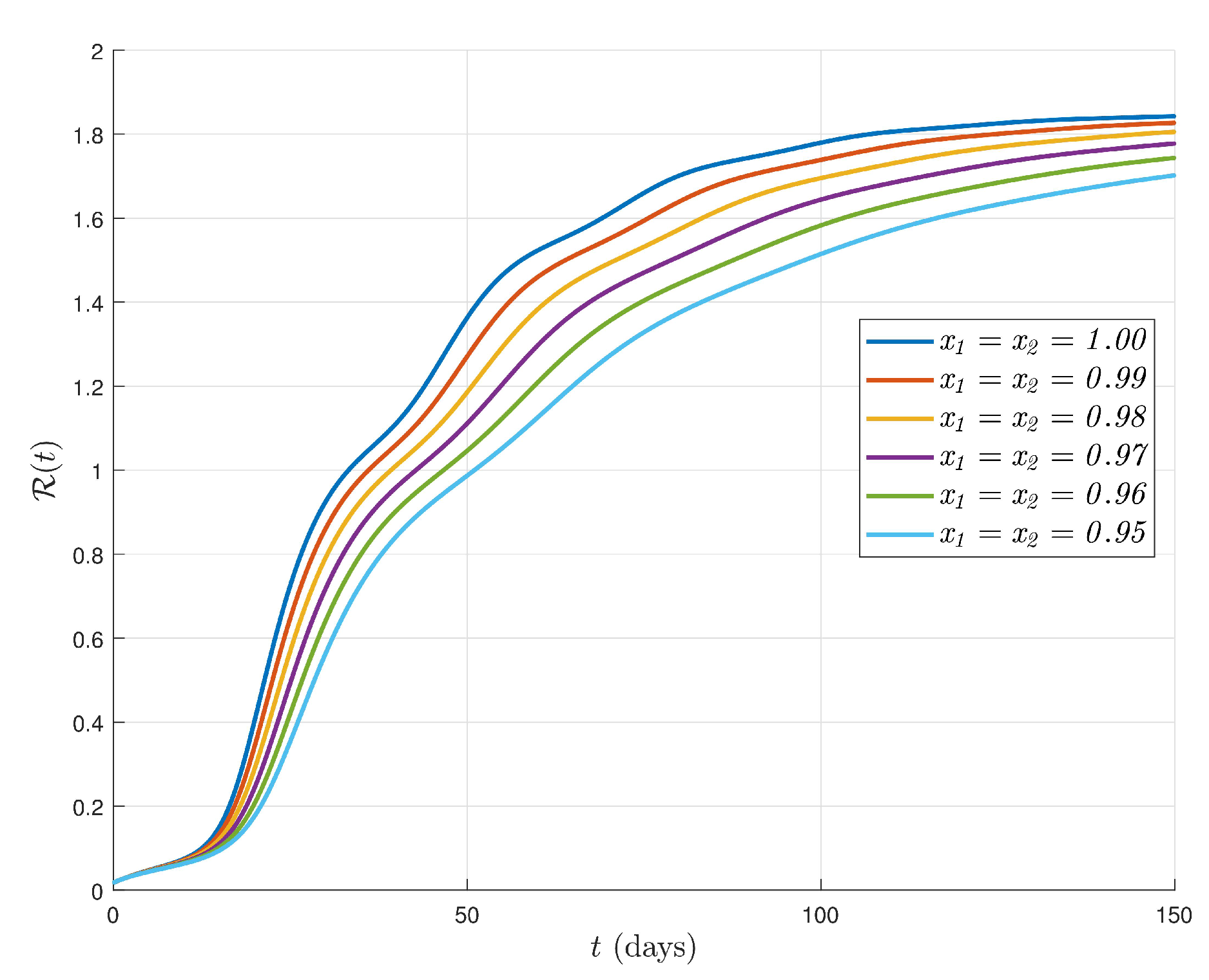
In view of the derivation of the model in Equation (3), the basic reproduction number, henceforth denoted as R 0 is expected to define the expected number of secondary cases produced, in a completely potential population, by a typical smoking individual [34]. Therefore, the progression from O to H and failure to quit smoking are not considered to be new cases, but rather the progression of a smoking individual through various compartments. Hence, the following results are stated. Moreover, time-dependent variations in the transmission potential of infectious diseases are of practical importance. Consequently, in Ref. [35] it is reported that time-dependent reproduction number R ( t ) measures the disease transmissibility, which can be estimated over the course of disease progression. Thus, R ( t ) has been particularly useful for monitoring epidemic trends by measuring the progress of interventions over time and for providing parameters for mathematical phenomena. Hence, by following [36], one can find the following results.
Theorem 9.
The time-dependent basic reproduction number for the fractal-fractional model of giving up smoking (3) is
R ( t ) = S ( t ) S ( 0 ) R 0 , w h e r e , R 0 = ω υ ϑ 2 .
Proof. 
It suffices to derive the R 0 . Then, the remaining part of the proof is followed easily. The respective vectors for the rate of appearance of new smokers and transfer of individuals in the model (3) are
F = ω P O 0 0 0 0 & V = ϑ P + ω P O υ ϑ O + γ O H ( ϑ + θ ) H γ O ( t ) H ( t ) ζ Q ( t ) ( ϑ + ζ ) Q ( t ) θ ( 1 q ) H ( t ) ϑ R ( t ) q θ H ( t ) . .
Based on the smoking compartments, i.e., O , H , Q and free-smoking equilibrium, we find that
F = ω υ ϑ 0 0 0 0 0 0 0 0 & V = ϑ 0 0 0 ( ϑ + θ ) ζ 0 θ ( 1 q ) ( ϑ + ζ ) .
It gives
V 1 = 1 ϑ [ ( ϑ + θ ) ( ϑ + ζ ) ζ θ ( 1 q ) ] ( ϑ + θ ) ( ϑ + ζ ) ζ θ ( 1 q ) 0 0 0 ϑ ( ϑ + ζ ) ϑ θ ( 1 q ) 0 ϑ ζ ϑ ( ϑ + ζ ) .
Thus, by Ref. [37], the basic reproduction number is followed easily. □

4.6. Sensitivity Analysis

In view of theorem 9, one can see that the sensitivity analysis of R ( t ) depends mainly on R 0 . Thus, in what follows, the analysis is therefore curtailed to the sensitivity of R 0 . By recalling that the sensitivity analysis enables us to predict which parameters have a high impact on the basic reproduction number [38], one of the main objectives is therefore to suggest strategies to ensure that the necessary control measures are taken to stop smoking and prevent a possible increase in the number of smokers in the future. Such attempts are, of course, attained in the direction of supporting the efforts of lowering the value of the basic reproduction number. Considering that there are many negative conditions brought about by smoking, together with the challenge of completely eliminating the smoking epidemic in a population in a short time, attempts to reduce the spread of smoking are therefore very important. Thus, lowering the value R 0 is one of the most fundamental issues, as it possesses a major influence on the effect of parameters on the change of R 0 . To this end, we will evaluate the influence aspects of the parameters that affect R 0 by determining the normalized forward sensitivity index of it [38]. Starting with the first to the last parameter listed under model in Equation (2), the normalized forward sensitivity index of the variable R 0 yields the following results.
Theorem 10.
The parameters γ , ζ , ϑ , q are likely to bring about the decrease in the time-dependent basic reproduction number.
Proof. 
It follows trivially through R 0 that
R 0 ω × ω R 0 = ω υ ϑ 2 ω × ω ω υ ϑ 2 = υ ϑ 2 ϑ 2 ω υ = ω 1 > 0 , R 0 γ × γ R 0 = ω υ ϑ 2 γ × γ ω υ ϑ 2 = 0 , R 0 ζ × ζ R 0 = ω υ ϑ 2 ζ × ζ ω υ ϑ 2 = 0 , R 0 ϑ × ϑ R 0 = ω υ ϑ 2 ϑ × ϑ ω υ ϑ 2 = 2 < 0 , R 0 θ × θ R 0 = ω υ ϑ 2 θ × θ ω υ ϑ 2 = 0 , R 0 q × q R 0 = ω υ ϑ 2 q × q ω υ ϑ 2 = 0 , R 0 υ × υ R 0 = ω υ ϑ 2 υ × υ ω υ ϑ 2 = ϑ 1 > 0 ,
which concludes the proof. □

4.7. Asymptotically Stability Analysis

To investigate the local asymptotic stability for the fractal-fractional model of giving up smoking (3), one requires the Jacobian matrix [39] computed at the equilibrium points and associated characteristic equation. Let E : = ( P ¯ , O ¯ , H ¯ , Q ¯ , R ¯ ) . Thus, the non-zero entries of the Jacobian matrix are
J ( E ) ( 1 , 1 ) = ( ϑ + ω O ¯ ) , J ( E ) ( 1 , 2 ) = ω P ¯ , J ( E ) ( 2 , 2 ) = ω P ¯ ϑ γ H ¯ , J ( E ) ( 3 , 2 ) = γ H ¯ , J ( E ) ( 3 , 3 ) = ( θ + ϑ ) , J ( E ) ( 3 , 4 ) = ζ , J ( E ) ( 4 , 3 ) = θ ( q 1 ) , J ( E ) ( 4 , 4 ) = ( ϑ + ζ ) , J ( E ) ( 5 , 3 ) = q θ , J ( E ) ( 5 , 5 ) = ϑ ,
and the associated characteristic equation [40] is
λ 5 a 4 λ 4 a 3 λ 3 a 2 λ 2 a 1 λ a 0 = 0 ,
where,
a 4 = γ O ¯ 5 ϑ ζ γ H ¯ θ ω O ¯ + ω P ¯ , a 3 = 4 O ¯ γ ϑ 4 ϑ ζ 10 ϑ 2 H ¯ γ θ 4 H ¯ γ ϑ H ¯ γ ζ 4 θ ϑ + O ¯ γ ζ O ¯ ω θ + P ¯ ω θ 4 O ¯ ω ϑ + 4 P ¯ ω ϑ O ¯ ω ζ + P ¯ ω ζ q θ ζ + O ¯ 2 γ ω H ¯ O ¯ γ ω O ¯ P ¯ γ ω , a 2 = 6 O ¯ γ ϑ 2 6 ϑ 2 ζ 10 ϑ 3 6 H ¯ γ ϑ 2 6 θ ϑ 2 6 O ¯ ω ϑ 2 + 6 P ¯ ω ϑ 2 + 3 O ¯ γ ϑ ζ 3 O ¯ ω θ ϑ + 3 P ¯ ω θ ϑ 3 O ¯ ω ϑ ζ + 3 P ¯ ω ϑ ζ 3 q θ ϑ ζ + 3 O ¯ 2 γ ω ϑ + O ¯ 2 γ ω ζ 3 H ¯ γ θ ϑ 3 H ¯ γ ϑ ζ H ¯ O ¯ γ ω θ 3 H ¯ O ¯ γ ω ϑ H ¯ O ¯ γ ω ζ 3 O ¯ P ¯ γ ω ϑ O ¯ P ¯ γ ω ζ H ¯ γ q θ ζ O ¯ ω q θ ζ + P ¯ ω q θ ζ , a 1 = 4 O ¯ γ ϑ 3 4 ϑ 3 ζ 5 ϑ 4 4 H ¯ γ ϑ 3 4 θ ϑ 3 4 O ¯ ω ϑ 3 + 4 P ¯ ω ϑ 3 3 H ¯ γ θ ϑ 2 3 H ¯ γ ϑ 2 ζ + 3 O ¯ γ ϑ 2 ζ 3 O ¯ ω θ ϑ 2 + 3 P ¯ ω θ ϑ 2 3 O ¯ ω ϑ 2 ζ + 3 P ¯ ω ϑ 2 ζ 3 q θ ϑ 2 ζ + 3 O ¯ 2 γ ω ϑ 2 3 H ¯ O ¯ γ ω ϑ 2 3 O ¯ P ¯ γ ω ϑ 2 + 2 O ¯ 2 γ ω ϑ ζ 2 H ¯ O ¯ γ ω θ ϑ 2 H ¯ O ¯ γ ω ϑ ζ 2 O ¯ P ¯ γ ω ϑ ζ 2 H ¯ γ q θ ϑ ζ 2 O ¯ ω q θ ϑ ζ + 2 P ¯ ω q θ ϑ ζ H ¯ O ¯ γ ω q θ ζ , a 0 = O ¯ γ ϑ 4 ϑ 4 ζ ϑ 5 H ¯ γ ϑ 4 θ ϑ 4 O ¯ ω ϑ 4 + P ¯ ω ϑ 4 H ¯ γ θ ϑ 3 H ¯ γ ϑ 3 ζ + O ¯ γ ϑ 3 ζ O ¯ ω θ ϑ 3 + P ¯ ω θ ϑ 3 O ¯ ω ϑ 3 ζ + P ¯ ω ϑ 3 ζ q θ ϑ 3 ζ + O ¯ 2 γ ω ϑ 3 + O ¯ 2 γ ω ϑ 2 ζ H ¯ O ¯ γ ω ϑ 3 O ¯ P ¯ γ ω ϑ 3 H ¯ O ¯ γ ω θ ϑ 2 H ¯ O ¯ γ ω ϑ 2 ζ O ¯ P ¯ γ ω ϑ 2 ζ H ¯ γ q θ ϑ 2 ζ O ¯ ω q θ ϑ 2 ζ + P ¯ ω q θ ϑ 2 ζ H ¯ O ¯ γ ω q θ ϑ ζ .
Thus, if
(a) 
5 ϑ + ζ + θ > ω υ ϑ ,
(b) 
q θ ζ + 4 ϑ ζ + 10 ϑ 2 + 4 θ ϑ > ( θ + 4 ϑ + ζ ) ω υ ϑ ,
(c)  
6 ϑ 2 ζ + 10 ϑ 3 + 6 θ ϑ 2 + 3 q θ ϑ ζ > ( 6 ϑ 2 + 3 θ ϑ + 3 ϑ ζ + q θ ζ ) ω υ ϑ ,
(d)  
4 ϑ 2 ζ + 5 ϑ 3 + 4 θ ϑ 2 + 3 q θ ϑ ζ > ( 4 ϑ 2 + 3 θ ϑ + 3 ϑ ζ + 2 q θ ζ ) ω υ ϑ ,
(e)  
ϑ 2 ζ + ϑ 3 + θ ϑ 2 + q θ ϑ ζ > ( ϑ 2 + θ ϑ + ϑ ζ + q θ ζ ) ω υ ϑ ,
in that case, the smoking-free equilibrium point is locally stable if the equilibrium points are positive [41].
Similarly, one finds that if
(a) 
5 ϑ + ζ + γ H ¯ + θ + ω O ¯ > γ O ¯ + ω P ¯ ,
(b)  
4 O ¯ ω ϑ + O ¯ ω ζ + q θ ζ + H ¯ O ¯ γ ω + O ¯ P ¯ γ ω + 4 ϑ ζ + 10 ϑ 2 + H ¯ γ θ + 4 H ¯ γ ϑ + H ¯ γ ζ + 4 θ ϑ + O ¯ ω θ > 4 O ¯ γ ϑ + O ¯ γ ζ + P ¯ ω θ + 4 P ¯ ω ϑ + P ¯ ω ζ + O ¯ 2 γ ω ,
(c)  
6 ϑ 2 ζ + 10 ϑ 3 + 6 H ¯ γ ϑ 2 + 6 θ ϑ 2 + 6 O ¯ ω ϑ 2 + 3 O ¯ ω θ ϑ + 3 O ¯ ω ϑ ζ + 3 q θ ϑ ζ + 3 H ¯ γ θ ϑ + 3 H ¯ γ ϑ ζ + H ¯ O ¯ γ ω θ + 3 H ¯ O ¯ γ ω ϑ + H ¯ O ¯ γ ω ζ + 3 O ¯ P ¯ γ ω ϑ + O ¯ P ¯ γ ω ζ + H ¯ γ q θ ζ + O ¯ ω q θ ζ > 6 O ¯ γ ϑ 2 + 6 P ¯ ω ϑ 2 + 3 O ¯ γ ϑ ζ + 3 P ¯ ω θ ϑ + 3 P ¯ ω ϑ ζ + 3 O ¯ 2 γ ω ϑ , + O ¯ 2 γ ω ζ + P ¯ ω q θ ζ ,
(d)  
4 ϑ 3 ζ + 5 ϑ 4 + 4 H ¯ γ ϑ 3 + 4 θ ϑ 3 + 4 O ¯ ω ϑ 3 + 3 H ¯ γ θ ϑ 2 + 3 H ¯ γ ϑ 2 ζ + 3 O ¯ ω θ ϑ 2 + 3 O ¯ ω ϑ 2 ζ + 3 q θ ϑ 2 ζ + 3 H ¯ O ¯ γ ω ϑ 2 + 3 O ¯ P ¯ γ ω ϑ 2 + 2 H ¯ O ¯ γ ω θ ϑ + 2 H ¯ O ¯ γ ω ϑ ζ + 2 O ¯ P ¯ γ ω ϑ ζ 2 H ¯ γ q θ ϑ ζ + 2 O ¯ ω q θ ϑ ζ + H ¯ O ¯ γ ω q θ ζ > 4 O ¯ γ ϑ 3 + 4 P ¯ ω ϑ 3 + 3 O ¯ γ ϑ 2 ζ + 3 P ¯ ω θ ϑ 2 + 3 P ¯ ω ϑ 2 ζ + 3 O ¯ 2 γ ω ϑ 2 + 2 O ¯ 2 γ ω ϑ ζ + 2 P ¯ ω q θ ϑ ζ ,
(e)  
ϑ 4 ζ + ϑ 5 + H ¯ γ ϑ 4 + θ ϑ 4 + O ¯ ω ϑ 4 + H ¯ γ θ ϑ 3 + H ¯ γ ϑ 3 ζ + O ¯ ω θ ϑ 3 + O ¯ ω ϑ 3 ζ + q θ ϑ 3 ζ + H ¯ O ¯ γ ω ϑ 3 + O ¯ P ¯ γ ω ϑ 3 + H ¯ O ¯ γ ω θ ϑ 2 + H ¯ O ¯ γ ω ϑ 2 ζ + O ¯ P ¯ γ ω ϑ 2 ζ + H ¯ γ q θ ϑ 2 ζ + O ¯ ω q θ ϑ 2 ζ + H ¯ O ¯ γ ω q θ ϑ ζ > O ¯ γ ϑ 4 + P ¯ ω ϑ 4 + O ¯ γ ϑ 3 ζ + P ¯ ω θ ϑ 3 + P ¯ ω ϑ 3 ζ + O ¯ 2 γ ω ϑ 3 + O ¯ 2 γ ω ϑ 2 ζ + P ¯ ω q θ ϑ 2 ζ ,
then the smoking equilibrium point is locally stable if the equilibrium points are positive [41].
Lemma 2.
The time-dependent basic reproduction number R ( t ) < 1 is globally stable in X , whereas, if R ( t ) > 1 , the unique smoking equilibrium point is globally asymptotically stable in the interior of X .
Proof. 
The proof of lemma 2 is similar to the proof established in [42]. □

5. Numerical Algorithm

In this section, we describe the numerical algorithm for the fractal-fractional model of giving up smoking (3). To do this, we apply the technique based on the fractal-fractional derivative operator [18]. To begin this process, we note that the system of fractal-fractional derivatives in the Riemann–Liouville sense in Equation (3) can be converted to
R L D 0 , t ϰ 1 P ( t ) = ϰ 2 τ ϰ 2 1 υ ϑ P ( t ) ω P ( t ) O ( t ) , R L D 0 , t ϰ 1 O ( t ) = ϰ 2 τ ϰ 2 1 ϑ O ( t ) + ω P ( t ) O ( t ) γ O ( t ) H ( t ) , R L D 0 , t ϰ 1 H ( t ) = ϰ 2 τ ϰ 2 1 ( ( ϑ + θ ) + γ O ( t ) ) H ( t ) + ζ Q ( t ) , R L D 0 , t ϰ 1 Q ( t ) = ϰ 2 τ ϰ 2 1 ( ϑ + ζ ) Q ( t ) + θ ( 1 q ) H ( t ) , R L D 0 , t ϰ 1 R ( t ) = ϰ 2 τ ϰ 2 1 ϑ R ( t ) + q θ H ( t ) .
By applying the Riemann–Liouville fractional integral on both sides of equation in (22) one obtains
P ( t ) = P ( 0 ) + ϰ 2 Γ ( ϰ 1 ) 0 t ι ϰ 2 1 ( t ι ) ϰ 1 1 υ ϑ P ( ι ) ω P ( ι ) O ( ι ) d ι , O ( t ) = O ( 0 ) + ϰ 2 Γ ( ϰ 1 ) 0 t ι ϰ 2 1 ( t ι ) ϰ 1 1 ϑ O ( ι ) + ω P ( ι ) O ( ι ) γ O ( ι ) H ( ι ) d ι , H ( t ) = H ( 0 ) + ϰ 2 Γ ( ϰ 1 ) 0 t ι ϰ 2 1 ( t ι ) ϰ 1 1 ( ( ϑ + θ ) + γ O ( ι ) ) H ( ι ) + ζ Q ( ι ) d ι , Q ( t ) = Q ( 0 ) + ϰ 2 Γ ( ϰ 1 ) 0 t ι ϰ 2 1 ( t ι ) ϰ 1 1 ( ϑ + ζ ) Q ( ι ) + θ ( 1 q ) H ( ι ) d ι , R ( t ) = R ( 0 ) + ϰ 2 Γ ( ϰ 1 ) 0 t ι ϰ 2 1 ( t ι ) ϰ 1 1 ϑ R ( ι ) + q θ H ( ι ) d ι .
Using a new approach at t n + 1 , (where n denotes the denotes the number of sub-intervals) we discretize the mentioned Equation (23) for t = t n + 1 , and we get
P ( t n + 1 ) = P 0 + ϰ 2 Γ ( ϰ 1 ) 0 t n + 1 ι ϰ 2 1 ( t n + 1 ι ) ϰ 1 1 υ ϑ P ( ι ) ω P ( ι ) O ( ι ) d ι , O ( t n + 1 ) = O 0 + ϰ 2 Γ ( ϰ 1 ) 0 t n + 1 ι ϰ 2 1 ( t n + 1 ι ) ϰ 1 1 ϑ O ( ι ) + ω P ( ι ) O ( ι ) γ O ( ι ) H ( ι ) d ι , H ( t n + 1 ) = H 0 + ϰ 2 Γ ( ϰ 1 ) 0 t n + 1 ι ϰ 2 1 ( t n + 1 ι ) ϰ 1 1 ( ( ϑ + θ ) + γ O ( ι ) ) H ( ι ) + ζ Q ( ι ) d ι , Q ( t n + 1 ) = Q 0 + ϰ 2 Γ ( ϰ 1 ) 0 t n + 1 ι ϰ 2 1 ( t n + 1 ι ) ϰ 1 1 ( ϑ + ζ ) Q ( ι ) + θ ( 1 q ) H ( ι ) d ι , R ( t n + 1 ) = R 0 + ϰ 2 Γ ( ϰ 1 ) 0 t n + 1 ι ϰ 2 1 ( t n + 1 ι ) ϰ 1 1 ϑ R ( ι ) + q θ H ( ι ) d ι .
Approximating the obtained integrals in Equation (24), we obtain
P ( t n + 1 ) = P 0 + ϰ 2 Γ ( ϰ 1 ) i = 0 n t i t i 1 ι ϰ 2 1 ( t n + 1 ι ) ϰ 1 1 υ ϑ P ( ι ) ω P ( ι ) O ( ι ) d ι , O ( t n + 1 ) = O 0 + ϰ 2 Γ ( ϰ 1 ) i = 0 n t i t i 1 ι ϰ 2 1 ( t n + 1 ι ) ϰ 1 1 ϑ O ( ι ) + ω P ( ι ) O ( ι ) γ O ( ι ) H ( ι ) d ι , H ( t n + 1 ) = H 0 + ϰ 2 Γ ( ϰ 1 ) i = 0 n t i t i 1 ι ϰ 2 1 ( t n + 1 ι ) ϰ 1 1 ( ( ϑ + θ ) + γ O ( ι ) ) H ( ι ) + ζ Q ( ι ) d ι , Q ( t n + 1 ) = Q 0 + ϰ 2 Γ ( ϰ 1 ) i = 0 n t i t i 1 ι ϰ 2 1 ( t n + 1 ι ) ϰ 1 1 ( ϑ + ζ ) Q ( ι ) + θ ( 1 q ) H ( ι ) d ι , R ( t n + 1 ) = R 0 + ϰ 2 Γ ( ϰ 1 ) i = 0 n t i t i 1 ι ϰ 2 1 ( t n + 1 ι ) ϰ 1 1 ϑ R ( ι ) + q θ H ( ι ) d ι .
Applying the Lagrangian piece-wise interpolation [43] to each functions
ι ϰ 2 1 ( t n + 1 ι ) ϰ 1 1 υ ϑ P ( ι ) ω P ( ι ) O ( ι ) , ι ϰ 2 1 ( t n + 1 ι ) ϰ 1 1 ϑ O ( ι ) + ω P ( ι ) O ( ι ) γ O ( ι ) H ( ι ) , ι ϰ 2 1 ( t n + 1 ι ) ϰ 1 1 ( ( ϑ + θ ) + γ O ( ι ) ) H ( ι ) + ζ Q ( ι ) , ι ϰ 2 1 ( t n + 1 ι ) ϰ 1 1 ( ϑ + ζ ) Q ( ι ) + θ ( 1 q ) H ( ι ) , ι ϰ 2 1 ( t n + 1 ι ) ϰ 1 1 ϑ R ( ι ) + q θ H ( ι ) ,
we find
ι ϰ 2 1 ( t n + 1 ι ) ϰ 1 1 υ ϑ P ( ι ) ω P ( ι ) O ( ι ) = ι t i 1 t i t i 1 t i ϰ 2 1 υ ϑ P ( t i ) ω P ( t i ) O ( t i ) ι t i t i t i 1 t i 1 ϰ 2 1 υ ϑ P ( t i 1 ) ω P ( t i 1 ) O ( t i 1 ) , ι ϰ 2 1 ( t n + 1 ι ) ϰ 1 1 ϑ O ( ι ) + ω P ( ι ) O ( ι ) γ O ( ι ) H ( ι ) = ι t i 1 t i t i 1 t i ϰ 2 1 ϑ O ( t i ) + ω P ( t i ) O ( t i ) γ O ( t i ) H ( t i ) ι t i t i t i 1 t i 1 ϰ 2 1 ϑ O ( t i 1 ) + ω P ( t i 1 ) O ( t i 1 ) γ O ( t i 1 ) H ( t i 1 ) , ι ϰ 2 1 ( t n + 1 ι ) ϰ 1 1 ( ( ϑ + θ ) + γ O ( ι ) ) H ( ι ) + ζ Q ( ι ) = ι t i 1 t i t i 1 t i ϰ 2 1 ( ( ϑ + θ ) + γ O ( t i ) ) H ( t i ) + ζ Q ( t i ) ι t i t i t i 1 t i 1 ϰ 2 1 ( ( ϑ + θ ) + γ O ( t i 1 ) ) H ( t i 1 ) + ζ Q ( t i 1 ) , ι ϰ 2 1 ( t n + 1 ι ) ϰ 1 1 ( ϑ + ζ ) Q ( ι ) + θ ( 1 q ) H ( ι ) = ι t i 1 t i t i 1 t i ϰ 2 1 ( ϑ + ζ ) Q ( t i ) + θ ( 1 q ) H ( t i ) ι t i t i t i 1 t i 1 ϰ 2 1 ( ϑ + ζ ) Q ( t i 1 ) + θ ( 1 q ) H ( t i 1 ) , ι ϰ 2 1 ( t n + 1 ι ) ϰ 1 1 ϑ R ( ι ) + q θ H ( ι ) = ι t i 1 t i t i 1 t i ϰ 2 1 ϑ R ( t i ) + q θ H ( t i ) ι t i t i t i 1 t i 1 ϰ 2 1 ϑ R ( t i 1 ) + q θ H ( t i 1 ) .
Consequently,
P ( t n + 1 ) = P 0 + ϰ 2 Γ ( ϰ 1 ) i = 0 n t i t i 1 ι ϰ 2 1 ( t n + 1 ι ) ϰ 1 1 [ ι t i 1 t i t i 1 t i ϰ 2 1 υ ϑ P ( t i ) ω P ( t i ) O ( t i ) ι t i t i t i 1 t i 1 ϰ 2 1 υ ϑ P ( t i 1 ) ω P ( t i 1 ) O ( t i 1 ) ] d ι , O ( t n + 1 ) = O 0 + ϰ 2 Γ ( ϰ 1 ) i = 0 n t i t i 1 ι ϰ 2 1 ( t n + 1 ι ) ϰ 1 1 ϑ O ( ι ) + ω P ( ι ) O ( ι ) γ O ( ι ) H ( ι ) d ι = ι t i 1 t i t i 1 t i ϰ 2 1 ϑ O ( t i ) + ω P ( t i ) O ( t i ) γ O ( t i ) H ( t i ) ι t i t i t i 1 t i 1 ϰ 2 1 ϑ O ( t i 1 ) + ω P ( t i 1 ) O ( t i 1 ) γ O ( t i 1 ) H ( t i 1 ) d ι , H ( t n + 1 ) = H 0 + ϰ 2 Γ ( ϰ 1 ) i = 0 n t i t i 1 ι ϰ 2 1 ( t n + 1 ι ) ϰ 1 1 ( ( ϑ + θ ) + γ O ( ι ) ) H ( ι ) + ζ Q ( ι ) d ι = ι t i 1 t i t i 1 t i ϰ 2 1 ( ( ϑ + θ ) + γ O ( t i ) ) H ( t i ) + ζ Q ( t i ) ι t i t i t i 1 t i 1 ϰ 2 1 ( ( ϑ + θ ) + γ O ( t i 1 ) ) H ( t i 1 ) + ζ Q ( t i 1 ) d ι , Q ( t n + 1 ) = Q 0 + ϰ 2 Γ ( ϰ 1 ) i = 0 n t i t i 1 ι ϰ 2 1 ( t n + 1 ι ) ϰ 1 1 ( ϑ + ζ ) Q ( ι ) + θ ( 1 q ) H ( ι ) d ι = ι t i 1 t i t i 1 t i ϰ 2 1 ( ϑ + ζ ) Q ( t i ) + θ ( 1 q ) H ( t i ) ι t i t i t i 1 t i 1 ϰ 2 1 ( ϑ + ζ ) Q ( t i 1 ) + θ ( 1 q ) H ( t i 1 ) d ι , R ( t n + 1 ) = R 0 + ϰ 2 Γ ( ϰ 1 ) i = 0 n t i t i 1 ι ϰ 2 1 ( t n + 1 ι ) ϰ 1 1 ϑ R ( t i ) + q θ H ( t i ) d ι ι t i t i t i 1 t i 1 ϰ 2 1 ϑ R ( t i 1 ) + q θ H ( t i 1 ) d ι .
The equations in (28) are equivalent to
P ( t n + 1 ) = P 0 + ϰ 2 ( Δ t ) ϰ 1 Γ ( ϰ 1 + 2 ) i = 0 n t i ϰ 2 1 υ ϑ P ( t i ) ω P ( t i ) O ( t i ) × [ ( n + 1 i ) ϰ 1 ( n i + 2 + ϰ 1 ) ( n i ) ϰ 1 ( n i + 2 + 2 ϰ 1 ) ] t i 1 ϰ 2 1 υ ϑ P ( t i 1 ) ω P ( t i 1 ) O ( t i 1 ) × [ ( n + 1 i ) ϰ 1 + 1 ( n i ) ϰ 1 ( n i + 1 + ϰ 1 ) ] ,
and
O ( t n + 1 ) = O 0 + ϰ 2 ( Δ t ) ϰ 1 Γ ( ϰ 1 + 2 ) i = 0 n t i ϰ 2 1 ϑ O ( t i ) + ω P ( t i ) O ( t i ) γ O ( t i ) H ( t i ) × [ ( n + 1 i ) ϰ 1 ( n i + 2 + ϰ 1 ) ( n i ) ϰ 1 ( n i + 2 + 2 ϰ 1 ) ] t i 1 ϰ 2 1 ϑ O ( t i 1 ) + ω P ( t i 1 ) O ( t i 1 ) γ O ( t i 1 ) H ( t i 1 ) × [ ( n + 1 i ) ϰ 1 + 1 ( n i ) ϰ 1 ( n i + 1 + ϰ 1 ) ] ,
and
H ( t n + 1 ) = H 0 + ϰ 2 ( Δ t ) ϰ 1 Γ ( ϰ 1 + 2 ) i = 0 n t i ϰ 2 1 ( ( ϑ + θ ) + γ O ( t i ) ) H ( t i ) + ζ Q ( t i ) × [ ( n + 1 i ) ϰ 1 ( n i + 2 + ϰ 1 ) ( n i ) ϰ 1 ( n i + 2 + 2 ϰ 1 ) ] t i 1 ϰ 2 1 ( ( ϑ + θ ) + γ O ( t i 1 ) ) H ( t i 1 ) + ζ Q ( t i 1 ) × [ ( n + 1 i ) ϰ 1 + 1 ( n i ) ϰ 1 ( n i + 1 + ϰ 1 ) ] ,
and
Q ( t n + 1 ) = Q 0 + ϰ 2 ( Δ t ) ϰ 1 Γ ( ϰ 1 + 2 ) i = 0 n t i ϰ 2 1 ( ϑ + ζ ) Q ( t i ) + θ ( 1 q ) H ( t i ) × [ ( n + 1 i ) ϰ 1 ( n i + 2 + ϰ 1 ) ( n i ) ϰ 1 ( n i + 2 + 2 ϰ 1 ) ] t i 1 ϰ 2 1 ( ϑ + ζ ) Q ( t i 1 ) + θ ( 1 q ) H ( t i 1 ) ] × [ ( n + 1 i ) ϰ 1 + 1 ( n i ) ϰ 1 ( n i + 1 + ϰ 1 ) ] ,
and
R ( t n + 1 ) = R 0 + ϰ 2 ( Δ t ) ϰ 1 Γ ( ϰ 1 + 2 ) i = 0 n t i ϰ 2 1 ϑ R ( t i ) + q θ H ( t i ) × [ ( n + 1 i ) ϰ 1 ( n i + 2 + ϰ 1 ) ( n i ) ϰ 1 ( n i + 2 + 2 ϰ 1 ) ] t i 1 ϰ 2 1 ϑ R ( t i 1 ) + q θ H ( t i 1 ) ] × [ ( n + 1 i ) ϰ 1 + 1 ( n i ) ϰ 1 ( n i + 1 + ϰ 1 ) ] .
We refer to equations in (29)–(33) as the numerical scheme for the solutions of the fractal-fractional model of giving up smoking (3).

6. Simulations and Discussion

Simulation and discussion on the behavior of the fractal-fractional model of giving up smoking (3) are implemented in this section according to the parameters computed in Ref. [14]. Based on this source, we assume υ = 0.2 , ϑ = 0.04 , γ = 0.3 , ζ = 0.25 , ω = 0.23 , θ = 2 , q = 0.4 . The initial values are:
P 0 = 0.60301 , O 0 = 0.24000 , H 0 = 0.10628 , Q 0 = 0.03260 , R 0 = 0.01811 .
As a first step, to compare the best fitting parameters with our assumption parameters [14], we regenerate the total population ( N = P + O + H + Q + R ) by adding white Gaussian noise. Then, we apply the well-known least square technique for the regenerated total population and find the curve of best fit for the new data. The comparative results including the approximate N ( t ) by the Adams–Bashforth technique (blue dashed line), regenerated N ( t ) with noise (blue dots), and the curve of best fit for the new data (red line) are graphically represented in Figure 1. From this graphical illustration, we can observe the great agreement between the Adams–Bashforth solution of N ( t ) and the curve of best fit created from the regenerated data with white Gaussian noise. In addition, obtained root mean square error for the best fit, which is a criterion to see the goodness of the fit, is produced as 0.3198 .
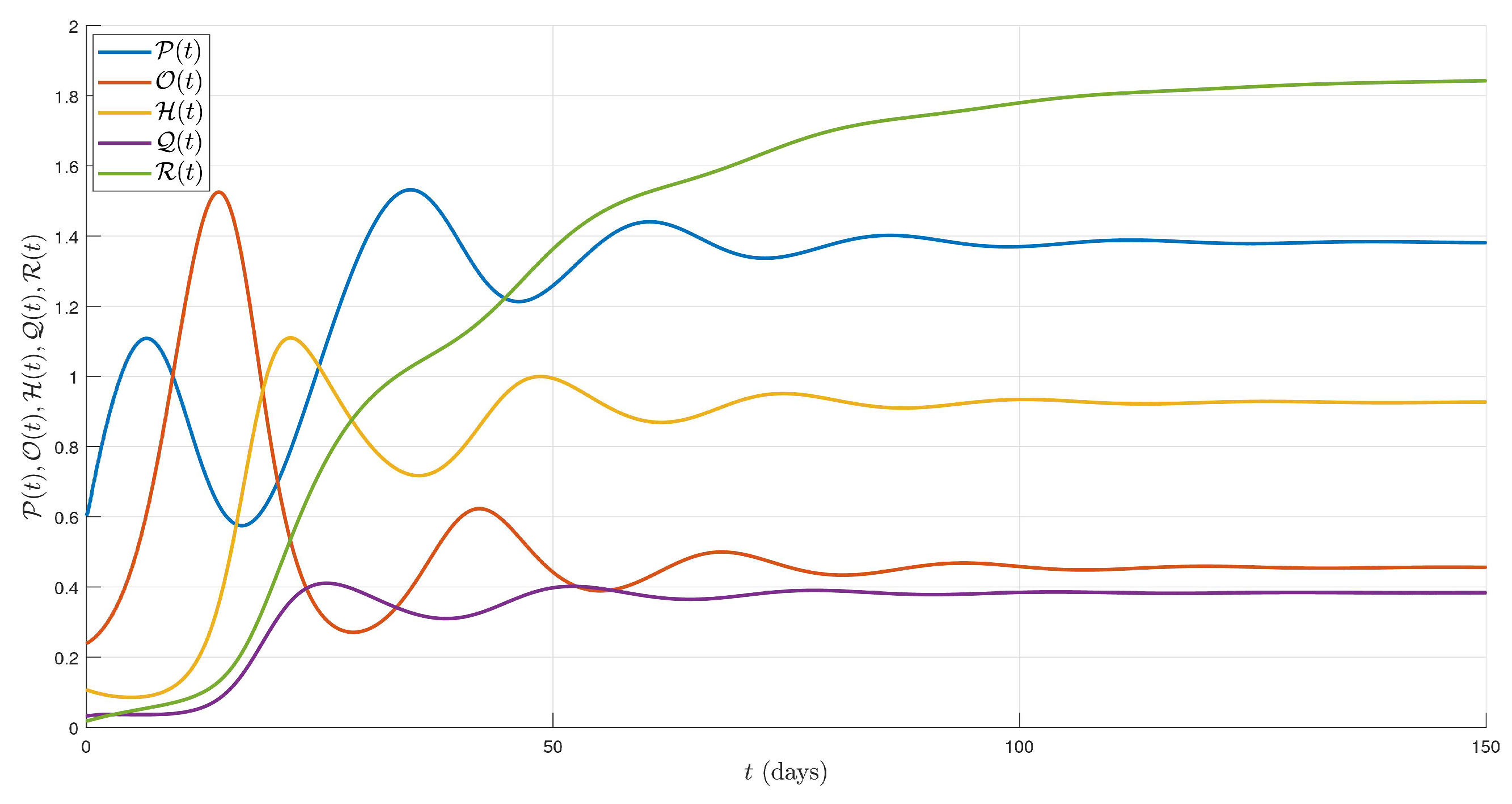
In Figure 2, we illustrate the obtained dynamics of all five state functions P , O , H , Q , R via the numerical technique introduced in Section 5.
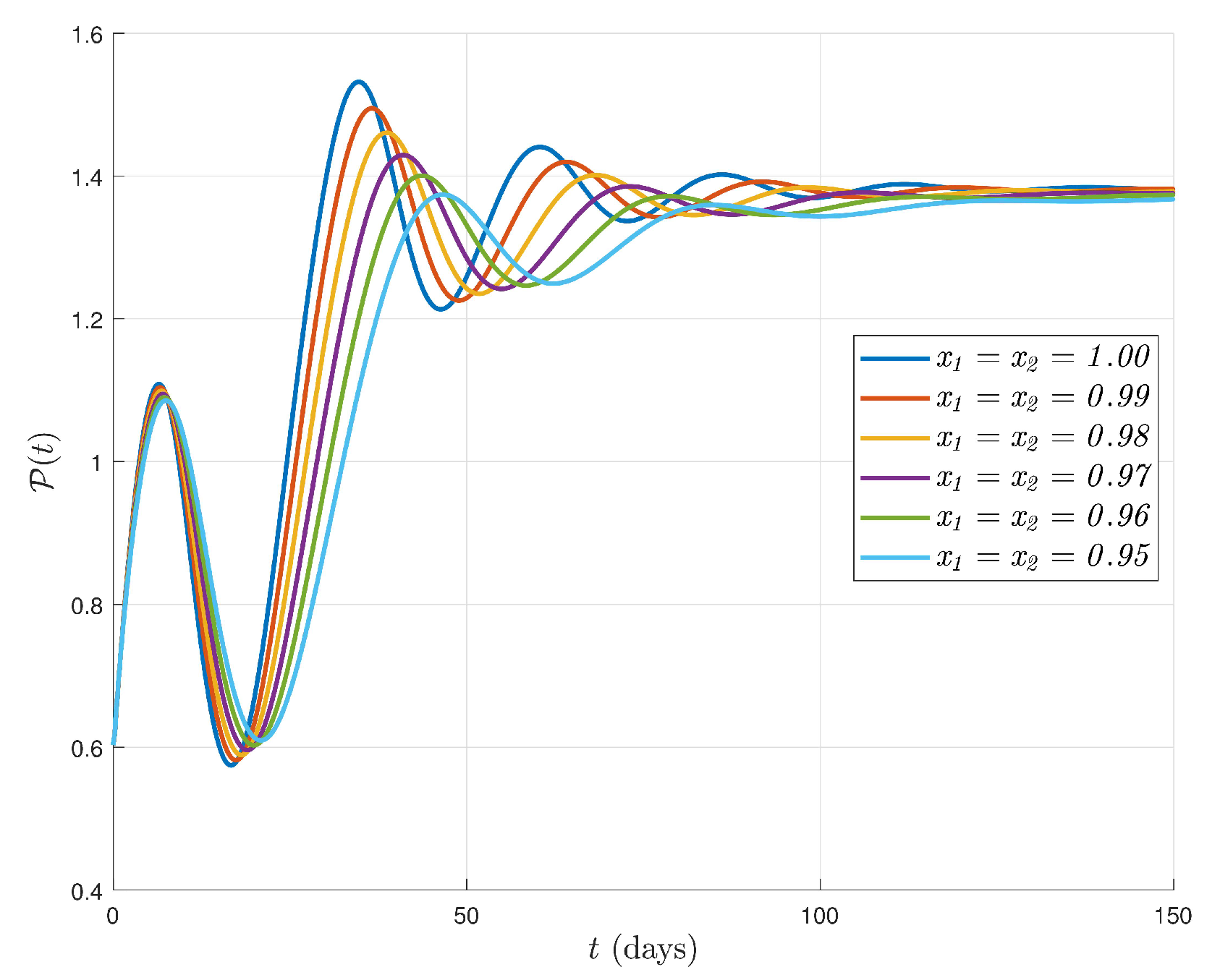
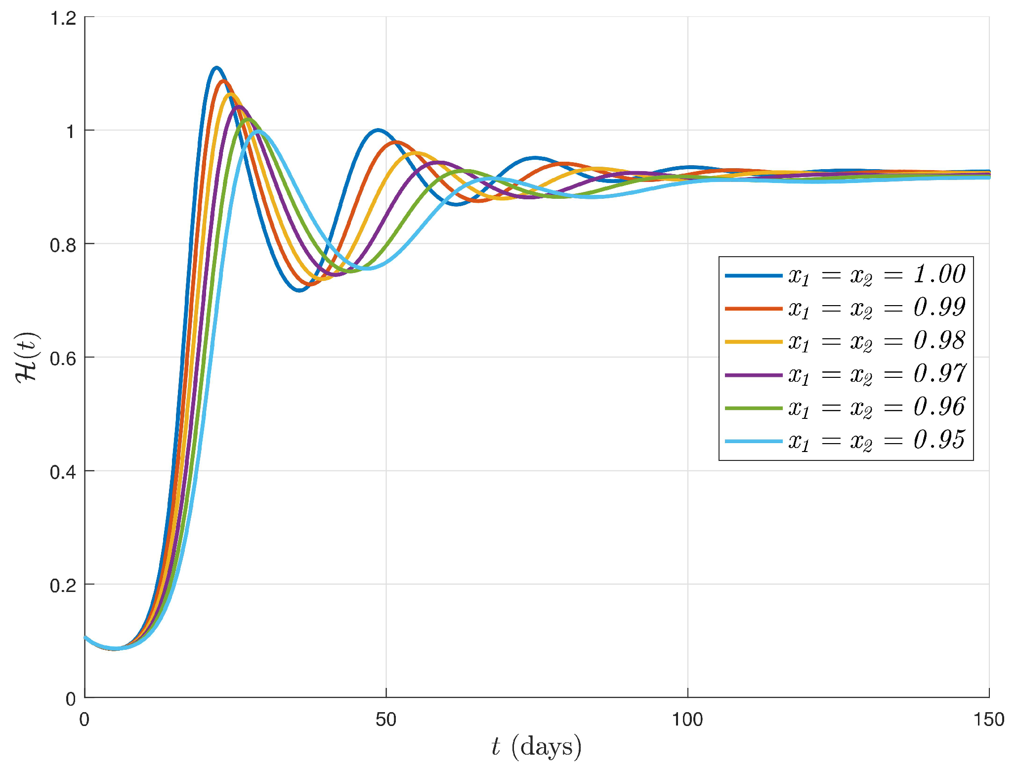
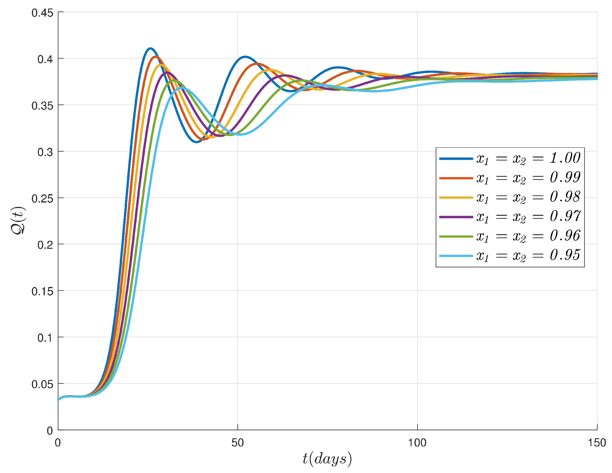
In Figure 3, Figure 4, Figure 5, Figure 6 and Figure 7, we illustrate the behaviors of five state functions P ( t ) , O ( t ) , H ( t ) , Q ( t ) , R ( t ) , respectively, when the Adams–Bashforth technique is applied under the fractal-fractional orders ϰ 1 = ϰ 2 = 0.95 , 0.96 , 0.97 , 0.98 , 1.00 . From these illustrations, we can observe that while the fractal-fractional order gets closer to the integer case, the density of each state function is increasing at about the same rate. In addition, it can be said that the fractal-fractional orders have an effect on the trajectories regarding converging to a more stable case.
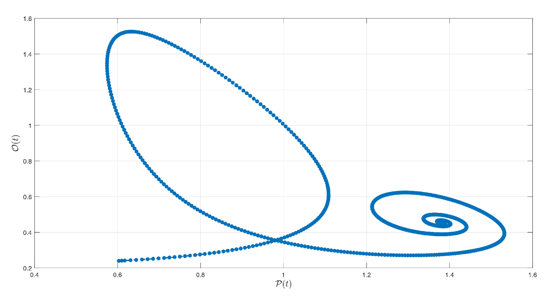
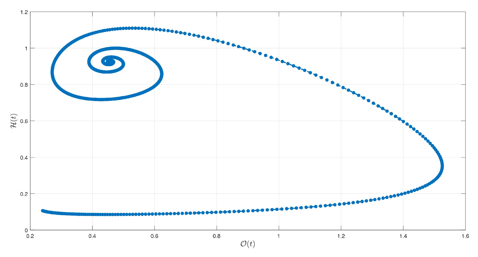
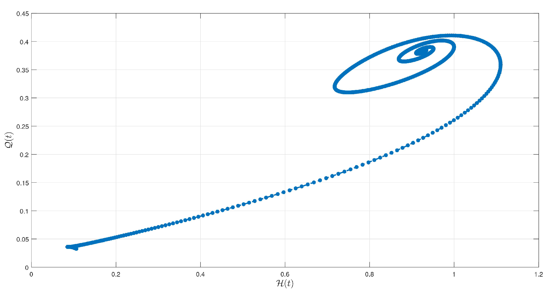
In Figure 8, Figure 9, Figure 10 and Figure 11, the behaviors of approximate solutions of some pairs of the state functions such as a) P ( t ) O ( t ) , b) P ( t ) R ( t ) , c) O ( t ) H ( t ) , and d) H ( t ) Q ( t ) under the integer-order are graphically illustrated where the time t [ 0 , 150 ] and step size h = 0.1 .
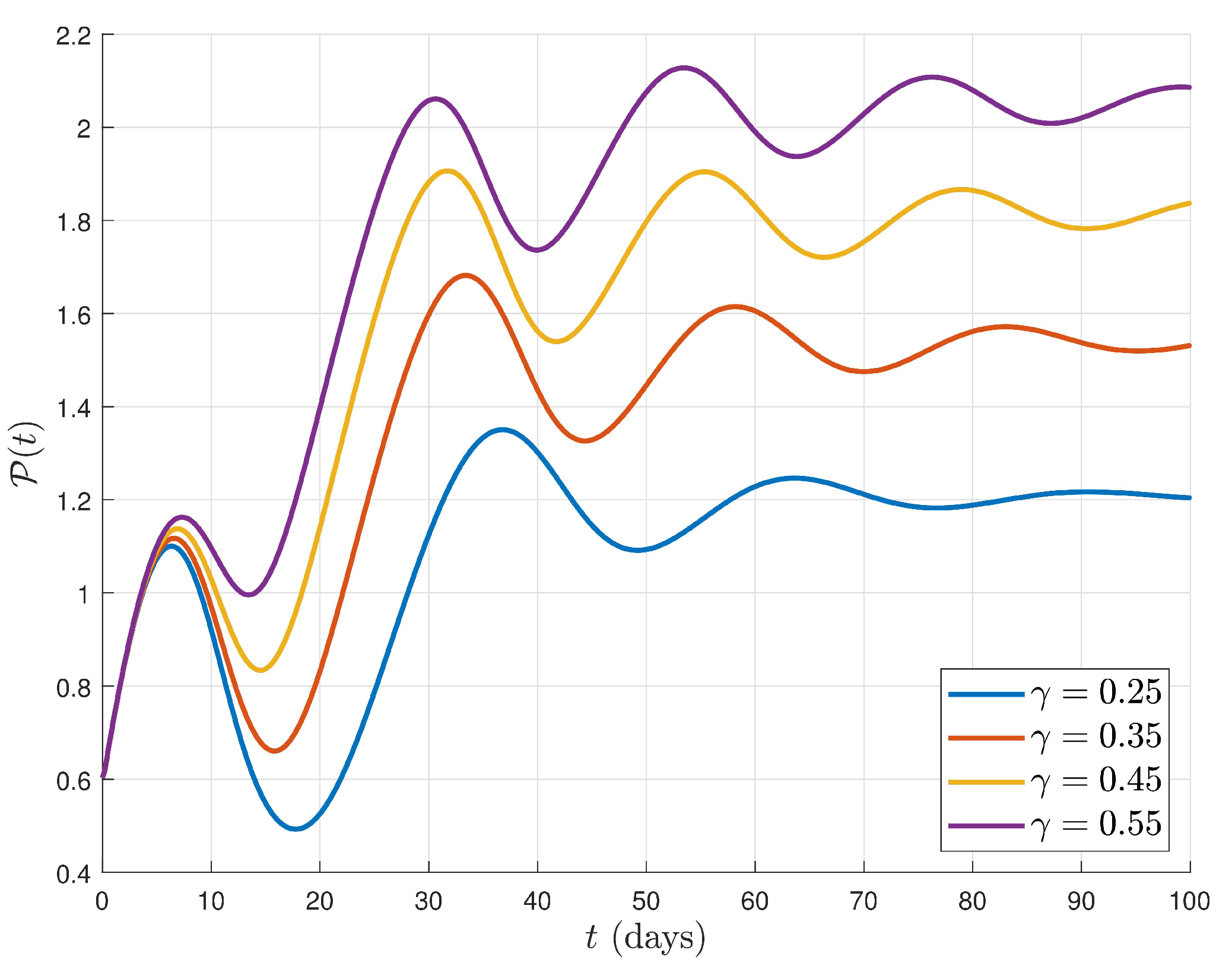
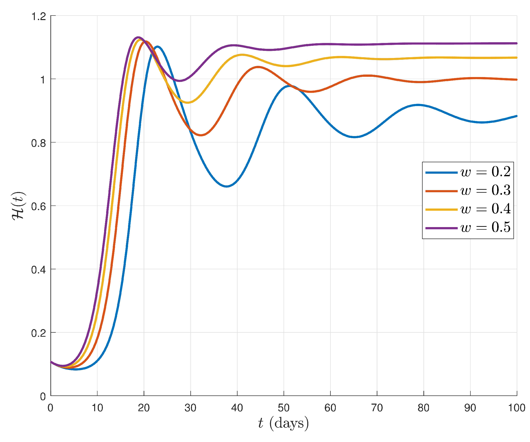
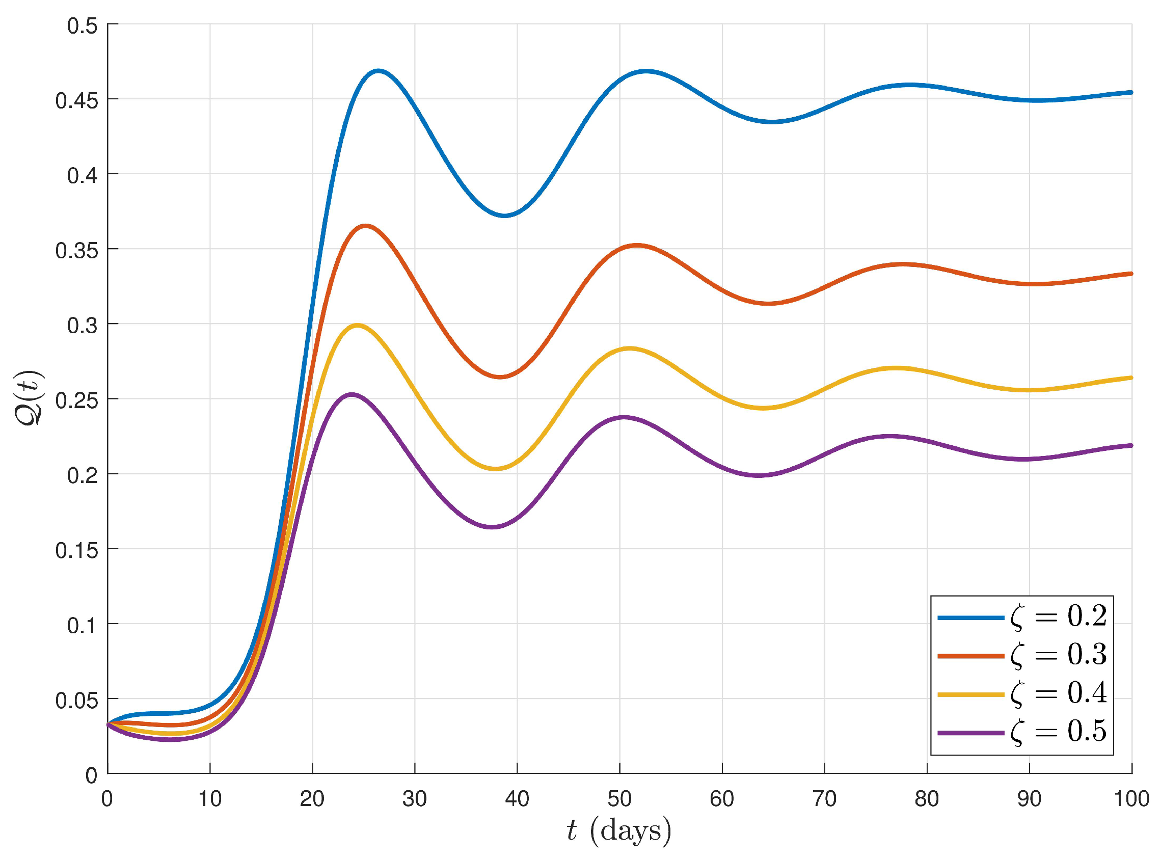
In Figure 12, Figure 13 and Figure 14, to observe the effects of contact rates on the sub-classes, we illustrate the behaviors of approximate solutions of state functions P ( t ) , H ( t ) and Q ( t ) versus the different values of contact rates γ , ω , ζ .
From Figure 12, we can observe that decreasing the contact rate between occasionally smokers and heavy smokers ( γ ) has a positive effect on the population of potential smokers P ; that is, the density of the potential smokers is decreasing at about the same rate. Similarly, when the contact rate between the potential smokers and occasional smokers ( ω ) decreases, from Figure 13, we can see that the population of heavy smokers H also decreases. Figure 14 shows us that increasing the contact rate between heavy smokers and temporary quitters who return back to smoking ( ζ ), has an effect on decreasing the population of temporary quitters who return back to smoking Q .

7. Conclusions

In this research, a new mathematical model of giving up smoking was designed by defining a five-compartmental system of differential equations based on the new hybrid generalized fractal-fractional derivatives. The properties of solutions to this fractal-fractional model of giving up smoking were discussed from several points of view. A special sub-class of increasing functions along with a special kind of contractions was used to complete the existing section about the solutions.Steady-state analysis was conducted for this model and we derived a numerical scheme for the fractal-fractional model of giving up smoking by terms of fractal and fractional parameters. In other words, we derived approximate solutions of the system (3) via the Adams–Bashforth method and simulated the behaviors of each sub-classes from several aspects such as variations of fractal-fractional dimension-orders. From the illustrated results, we can see that by increasing the fractal-fractional orders, the density of each sub-population also increases. We also observed and discussed the effects of contact rates γ , ω , ζ on the behaviors of sub-classes in Section 6. All the approximate results and calculations are obtained with the help of MATLAB version R2019A. These simulations and graphs show that if we control the contact rate in each sub-class, then we can obtain significant results in reducing the number of people who quit smoking. New directions can be extended by considering other generalized kernels in the fractal-fractional operators in future research projects.

Author Contributions

Conceptualization, S.E., S.R. and R.P.A.; formal analysis, S.E., A.S., K.M.O., B.T., İ.A., S.R. and R.P.A.; methodology, S.E., A.S., K.M.O., B.T., İ.A., S.R. and R.P.A.; software, S.E., K.M.O. and İ.A. All authors have read and agreed to the published version of the manuscript.

Funding

This research received no funding.

Institutional Review Board Statement

Not applicable.

Informed Consent Statement

Not applicable.

Data Availability Statement

Data sharing is not applicable to this article as no datasets were generated nor analyzed during the current study.

Acknowledgments

The first and sixth authors would like to thank Azarbaijan Shahid Madani University. The second author would like to thank University of Namibia. In addition, the third author author would like to thank Federal University of Technology Akure.

Conflicts of Interest

The authors declare no conflict of interest.

References

  1. Zaman, G. Qualitative behavior of giving up smoking models. Bull. Malays. Math. Soc. 2011, 34, 403–415. [Google Scholar]
  2. Sharomi, O.; Gumel, A.B. Curtailing smoking dynamics: A mathematical modeling approach. Appl. Math. Comput. 2008, 195, 475–499. [Google Scholar] [CrossRef]
  3. Alkhudhari, Z.; Al-Sheikh, S.; Al-Tuwairqi, S. Global dynamics of a mathematical model on smoking. Appl. Math. 2014, 2014, 847075. [Google Scholar] [CrossRef]
  4. Rahman, G.U.; Agarwal, R.P.; Liu, L.; Khan, A. Threshold dynamics and optimal control of an age-structured giving up smoking model. Nonlinear Anal. Real World Appl. 2018, 43, 96–120. [Google Scholar] [CrossRef]
  5. Rahman, G.U.; Agarwal, R.P.; Din, Q. Mathematical analysis of giving up smoking model via harmonic mean type incidence rate. Appl. Math. Comput. 2019, 354, 128–148. [Google Scholar] [CrossRef]
  6. Zhang, Z.; Rahman, G.U.; Agarwal, R.P. Harmonic mean type dynamics of a delayed giving up smoking model and optimal control strategy via legislation. J. Franklin Ins. 2020, 357, 10669–10690. [Google Scholar] [CrossRef]
  7. Li, X.; Agarwal, R.P.; Gomez-Aguilar, J.F.; Badshah, Q.; Rahman, G.U. Threshold dynamics: Formulation, stability & sensitivity analysis of co-abuse model of heroin and smoking. Chaos Solitons Fractals 2022, 161, 112373. [Google Scholar]
  8. Caputo, M.; Fabrizio, M. A new definition of fractional derivative without singular kernel. Prog. Fract. Differ. Appl. 2015, 1, 73–85. [Google Scholar]
  9. Atangana, A.; Baleanu, D. New fractional derivatives with non-local and non-singular kernel: Theory and application to heat transfer model. Therm. Sci. 2016, 20, 763–769. [Google Scholar] [CrossRef] [Green Version]
  10. Podlubny, I. Fractional Differential Equations; Academic Press: Cambridge, MA, USA, 1999. [Google Scholar]
  11. Erturk, V.S.; Zaman, G.; Momani, S. A numeric analytic method for approximating a giving up smoking model containing fractional derivatives. Comput. Math. Appl. 2012, 64, 3068–3074. [Google Scholar] [CrossRef] [Green Version]
  12. Zaman, G.; Islam, S. A non-standard numerical method for a giving-up smoking model. Nonlinear Sci. Lett. A 2010, 4, 397–402. [Google Scholar]
  13. Zeb, A.; Chohan, I.; Zaman, G. The homotopy analysis method for approximating of giving up smoking model in fractional order. Appl. Math. 2012, 3, 914–919. [Google Scholar] [CrossRef]
  14. Singh, J.; Kumar, D.; Qurashi, M.A.; Baleanu, D. A new fractional model for giving up smoking dynamics. Adv. Differ. Equ. 2017, 2017, 88. [Google Scholar] [CrossRef] [Green Version]
  15. Ahmad, A.; Farman, M.; Ghafar, A.; Inc, M.; Ahmad, M.O.; Sene, N. Analysis and simulation of fractional order smoking epidemic model. Comput. Math. Meth. Med. 2022, 2022, 9683187. [Google Scholar] [CrossRef] [PubMed]
  16. Ucar, S.; Ucar, E.; Ozdemir, N.; Hammouch, Z. Mathematical analysis and numerical simulation for a smoking model with Atangana–Baleanu derivative. Chaos Solitons Fractals 2019, 118, 300–306. [Google Scholar] [CrossRef]
  17. Atangana, A. Fractal-fractional differentiation and integration: Connecting fractal calculus and fractional calculus to predict complex system. Chaos Solitons Fractals 2017, 102, 396–406. [Google Scholar] [CrossRef]
  18. Atangana, A.; Qureshi, S. Modeling attractors of chaotic dynamical systems with fractal-fractional operators. Chaos Solitons Fractals 2019, 123, 320–337. [Google Scholar] [CrossRef]
  19. Khan, H.; Ahmad, F.; Tunc, O.; Idrees, M. On fractal-fractional Covid-19 mathematical model. Chaos Solitons Fractals 2022, 157, 111937. [Google Scholar] [CrossRef]
  20. Khan, H.; Alzabut, J.; Shah, A.; Etemad, S.; Rezapour, S.; Park, C. A study on the fractal-fractional tobacco smoking model. AIMS Math. 2022, 7, 13887–13909. [Google Scholar] [CrossRef]
  21. Najafi, H.; Etemad, S.; Patanarapeelert, N.; Asamoah, J.K.K.; Rezapour, S.; Sitthiwirattham, T. A study on dynamics of CD4+ T-cells under the effect of HIV-1 infection based on a mathematical fractal-fractional model via the Adams-Bashforth scheme and Newton polynomials. Mathematics 2022, 10, 1366. [Google Scholar] [CrossRef]
  22. Abro, K.A.; Atangana, A. Numerical and mathematical analysis of induction motor by means of AB-fractal-fractional differentiation actuated by drilling system. Numer. Meth. Partial Differ. Equ. 2022, 38, 293–307. [Google Scholar] [CrossRef]
  23. Saad, K.M.; Alqhtani, M.; Gomez-Aguilar, J.F. Fractal-fractional study of the hepatitis C virus infection model. Res. Phys. 2020, 19, 103555. [Google Scholar] [CrossRef]
  24. Etemad, S.; Avcı, İ.; Kumar, P.; Baleanu, D.; Rezapour, S. Some novel mathematical analysis on the fractal–fractional model of the AH1N1/09 virus and its generalized Caputo-type version. Chaos Solitons Fractals 2022, 162, 112511. [Google Scholar] [CrossRef]
  25. Asamoah, J.K.K. Fractal-fractional model and numerical scheme based on Newton polynomial for Q fever disease under Atangana-Baleanu derivative. Res. Phys. 2022, 34, 105189. [Google Scholar] [CrossRef]
  26. Khan, H.; Alam, K.; Gulzar, H.; Etemad, S.; Rezapour, S. A case study of fractal-fractional tuberculosis model in China: Existence and stability theories along with numerical simulations. Math. Comput. Simul. 2022, 198, 455–473. [Google Scholar] [CrossRef]
  27. Mohammadi, H.; Kumar, S.; Rezapour, S.; Etemad, S. A theoretical study of the Caputo-Fabrizio fractional modeling for hearing loss due to Mumps virus with optimal control. Chaos Solitons Fractals 2021, 144, 110668. [Google Scholar] [CrossRef]
  28. Owolabi, K.M.; Shikongo, A. Fractal Fractional Operator Method on HER2+ Breast Cancer Dynamics. Int. J. Appl. Comput. Math. 2021, 7, 85. [Google Scholar] [CrossRef]
  29. Owolabi, K.M.; Shikongo, A.; Atangana, A. Fractal Fractional Derivative Operator Method on MCF-7 Cell Line Dynamics. In Methods of Mathematical Modelling and Computation for Complex Systems. Studies in Systems, Decision and Control; Singh, J., Dutta, H., Kumar, D., Baleanu, D., Hristov, J., Eds.; Springer: Cham, Switzerland, 2022; Volume 373. [Google Scholar]
  30. Samet, B.; Vetro, C.; Vetro, P. Fixed point theorems for α-ψ-contractive type mappings. Nonlinear Anal. 2012, 75, 2154–2165. [Google Scholar] [CrossRef] [Green Version]
  31. Granas, A.; Dugundji, J. Fixed Point Theory; Springer: New York, NY, USA, 2003. [Google Scholar]
  32. Rassias, T.M. On the stability of the linear mapping in Banach spaces. Proc. Amer. Math. Soc. 1978, 72, 297–300. [Google Scholar] [CrossRef]
  33. Cho, Y.J.; Park, C.; Rassias, T.M.; Saadati, R. Stability of Functional Equations in Banach Algebras; Springer: Cham, Switzerland, 2015. [Google Scholar]
  34. den Driessche, P.V.; Watmough, J. Reproduction numbers and sub-threshold endemic equilibria for compartmental models of disease transmission. Math. Biosci. 2002, 180, 29–48. [Google Scholar] [CrossRef]
  35. Arruda, A.G.; Alkhamis, M.A.; VanderWaal, K.; Morrison, R.B.; Perez, A.M. Estimation of time-dependent reproduction numbers for porcine reproductive and respiratory syndrome across different regions and production systems of the US. Front. Vet. Sci. 2017, 4, 46. [Google Scholar] [CrossRef] [PubMed] [Green Version]
  36. Diekmann, O.; Heesterbeek, J.A.P. Mathematical Epidemiology of Infectious Diseases; Model Building, Analysis and Interpretation; John Wiley and Sons: New York, NY, USA, 2000. [Google Scholar]
  37. Diekmann, O.; Heesterbeek, J.A.P.; Metz, J.A.J. On the definition and the computation of the basic reproduction ratio R0 in models for infectious diseases in heterogeneous populations. J. Math. Biol. 1990, 28, 365–382. [Google Scholar] [CrossRef] [Green Version]
  38. Chitnis, N.; Hyman, J.M.; Cushing, J.M. Determining important parameters in the spread of malaria through the sensitivity analysis of a mathematical model. Bull. Math. Biol. 2008, 70, 1272–1296. [Google Scholar] [CrossRef]
  39. Mathai, A.M. Jobians of Matrix Transformation and Functions of Matrix Arguments; World Scientific Publishing: Hackensack, NJ, USA, 1997. [Google Scholar]
  40. Bretscher, O. Linear Algebra with Applications-Pearson; Cambridge University Press: New York, NY, USA, 1974. [Google Scholar]
  41. Kim, J.-H.; Su, W.; Song, Y.J. On stability of a polynomial. J. Appl. Math. Inform. 2018, 36, 231–236. [Google Scholar]
  42. Li, M.Y.; Wang, L. Global stability in some seir epidemic models. In Mathematical Approaches for Emerging and Reemerging Infectious Diseases: Models, Methods, and Theory; Castillo-Chavez, C., Blower, S., van den Driessche, P., Kirschner, D., Yakubu, A.A., Eds.; Springer: New York, NY, USA, 2002. [Google Scholar]
  43. Burden, R.L.; Faires, J.D. Numerical Analysis; Brooks/Cole: Pacific Grove, CA, USA, 2011. [Google Scholar]
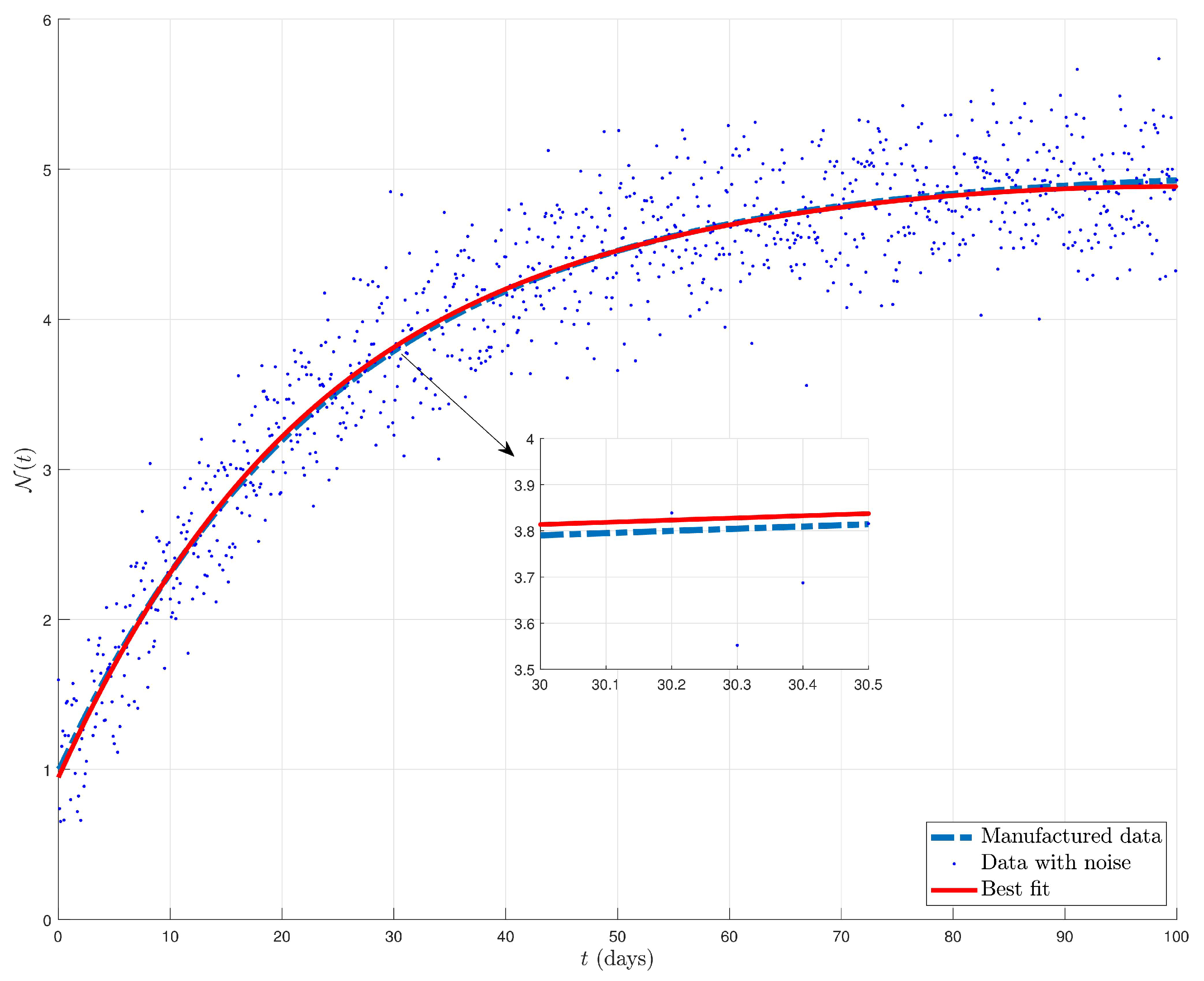
Figure 1. Comparison between the approximate total population N ( t ) with noise data and curve of best fit.
Mathematics 10 04369 g001
Figure 2. Behaviors of five sub-classes under fractal-fractional order ϰ 1 = ϰ 2 = 1.00 .
Mathematics 10 04369 g002
Figure 3. Behaviors of P ( t ) .
Mathematics 10 04369 g003
Figure 4. Behaviors of O ( t ) .
Mathematics 10 04369 g004
Figure 5. Behaviors of H ( t ) .
Mathematics 10 04369 g005
Figure 6. Behaviors of Q ( t ) .
Mathematics 10 04369 g006
Figure 7. Behaviors of R ( t ) .
Mathematics 10 04369 g007
Figure 8. Behaviors of pair of sub-classes P ( t ) O ( t ) .
Mathematics 10 04369 g008
Figure 9. Behaviors of pair of sub-classes P ( t ) R ( t ) .
Mathematics 10 04369 g009
Figure 10. Behaviors of pair of sub-classes O ( t ) H ( t ) .
Mathematics 10 04369 g010
Figure 11. Behaviors of pair of sub-classes H ( t ) Q ( t ) .
Mathematics 10 04369 g011
Figure 12. Effects of contact rates on state functions: P ( t ) versus γ .
Mathematics 10 04369 g012
Figure 13. Effects of contact rates on state functions: H ( t ) versus ω .
Mathematics 10 04369 g013
Figure 14. Effects of contact rates on state functions: Q ( t ) versus ζ .
Mathematics 10 04369 g014
Publisher’s Note: MDPI stays neutral with regard to jurisdictional claims in published maps and institutional affiliations.