Smart Patrolling Based on Spatial-Temporal Information Using Machine Learning

Abstract

With the aim of improving security in cities and reducing the number of crimes, this research proposes an algorithm that combines artificial intelligence (AI) and machine learning (ML) techniques to generate police patrol routes. Real data on crimes reported in Quito City, Ecuador, during 2017 are used. The algorithm, which consists of four stages, combines spatial and temporal information. First, crimes are grouped around the points with the highest concentration of felonies, and future hotspots are predicted. Then, the probability of crimes committed in any of those areas at a time slot is studied. This information is combined with the spatial way-points to obtain real surveillance routes through a fuzzy decision system, that considers distance and time (computed with the OpenStreetMap API), and probability. Computing time has been analized and routes have been compared with those proposed by an expert. The results prove that using spatial–temporal information allows the design of patrolling routes in an effective way and thus, improves citizen security and decreases spending on police resources.

1. Introduction

Citizen insecurity is a serious problem in all countries, especially in Latin America and the Caribbean, which have higher rates of criminal events, great insecurity, and a profound deterioration of trust in citizen surveillance institutions, such as the police and the army. An example of this situation is the prevalence of endemic levels of violence, where homicide rates have been growing steadily over time. The rate of homicides has remarkably increased from 25.9% in 2017 to 30% in 2020 in Central America and from 24.2% in 2017 to 29% in 2020 in South America [1].

Criminal events increase due to unemployment, social and economic problems, among other reasons. Ecuador is one of the countries with a rising crime rate, even though the National Police carries out a continuous surveillance of sectors with high crime incidences to reduce this problem. The homicide rate in Ecuador was 5.78% in 2017 and 7.78% in 2020, which represents a relevant increase [2].

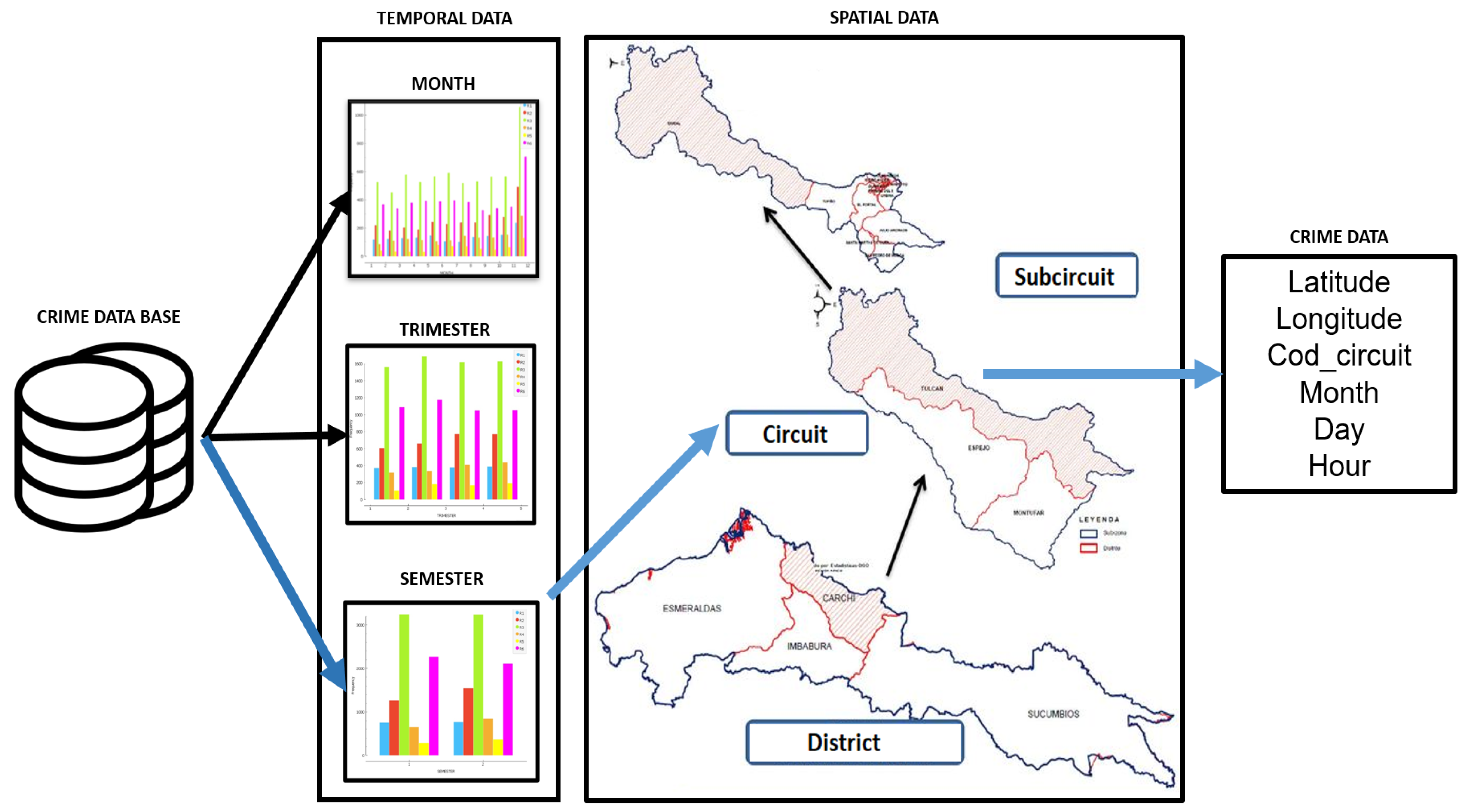
With the motivation of improving citizen security, this study proposes an algorithm for forecasting locations with a high probability of crime. This prediction is then used for the generation of patrol routes in a given area. A database with spatial–temporal information of the crimes that occurred in Quito City, Ecuador, from January to December 2017 is used.

The patrol route planning is a complex problem as it involves location, hotspots, manpower, and scheduling of vehicles and human resources. To deal with it, the application of several computational methods to develop efficient algorithms is required. The combination of various artificial intelligence (AI) and machine learning (ML) techniques has proven effective in decision-making applications in diverse settings [3,4]. That is the strategy proposed in this research, that has provided succesful results in this specific application.

The hybrid system here designed combines some intelligent data processing techniques for decision making. First, geographic data from the most conflictive areas regarding crimes are grouped using the k-means clustering algorithm. Statistical methods are then used to identify critical points in each region defined by a cluster, and linear regression functions are used for the prediction of future crime points. Subsequently, an analysis of the probability of the occurrence of crimes is carried out according to geographical location and temporal information available. With this information, fuzzy logic is applied so to consider several criteria in the drawing of the patrol route. The algorithm has been tested on various real-world scenarios, with useful and satisfactory results. This strategy provides relevant information for the management of police resources, which allows better use of these means and the reduction of urban crimes.

The novelty of the proposal consists of showing how some well-known intelligent techniques are configured and combined to develop an efficient tool for patrol route generation. It has been proved in several fields that hybrid systems are necessary to address the complexity of real problems. In this work, the sequence of activities is key to design the route generation algorithm, together with the consideration of spacial-temporal information. The main contributions of this article can be then summarized as follows: (1) Geographic segmentation of crimes to obtain points with high crime rates (hotspots) in an automatic way. (2) Forecasting of future spatial crime locations based on historic information. (3) Design of optimal patrol routes based on crime probability considering spatio-temporal data. Fuzzy logic uses distance and travel time between surveillance way-points to minimize resources cost and response time emergencies.

The structure of the paper is as follows. In Section 2 some relevant related works on crime data analysis are discussed. The materials and methods used are described in Section 3. Section 4 and Section 5 detail the flow and operation of the algorithm, as well as the application of ML and statistical techniques. In Section 6, simulation results and analysis of the data obtained are presented. The paper ends with the conclusions and future lines of research.

2. Related Works

The analysis and prediction of crimes have raised great interest because of their usefulness in improving citizen security. This topic has been approached from different points of view. Regression and AI techniques have been frequently applied although papers suing space–time information are not so common. To mention some examples, in the research developed by [5], the crimes forecasting is done by applying a deep neural network architecture, identifying evolutionary patterns of crimes and the relationship between space–time information. Crime points (geospatial) are then transformed into crime heat maps for the same sector of a city and time. Subsequently, convolutional hierarchical structures are applied to train a crime prediction model with heat maps. Esquivel  [6] applied convolutional neural networks and a short- and a long-term memory network for crime prediction in the city of Baltimore, USA. It uses spatial and temporal correlations of historical crime data for future predictions. An inspirational paper was the one by Farjami [7], who proposed a genetic-fuzzy algorithm for spatial-temporal crime prediction. First, available information is processed, which consists of the geographical location (latitude, longitude) and the time of crimes. Then, a forecasting model is built to determine the time and place where future crimes will occur. Finally, the model is evaluated with simulated data from the city of Tehran, Iran. Hu [8] applied Bayesian spatial–temporal modeling for urban crime and analyzed its trend in the city of Wuhan, China. It uses socio-economic and population variables such as people agglomeration places, unemployment, tourist and residential places, and so on. Vural [9] used the Naïve Bayes theory to identify an offender with the highest probability of executing a criminal act based on the deliquent’s history. The information conveyed is the date, geographical location, type, and some crime data. The proposed model works with a georeferenced information system that visualizes various characteristics of crimes and identifies patterns on a defined territory. Win [10] proposed a fuzzy grouping algorithm of criminal activities to detect patterns of criminal behavior. This algorithm predicts hotspots by using geospatial information in various cities in Iraq, Pakistan, Afghanistan, and India.

Regression is also commonly applied in this area. An interesting related paper is the one by Catlett [11], who applied auto regressive models on spatial–temporal information to automatically identify high-risk crime regions in highly populated urban areas. A spatial grouping of the dataset is carried out to detect these regions of high crime density. Finally, an integrated moving average auto-regressive prediction model is generated to forecast the reliably forecast crime trends in each region. Kadar [12] used space–time, socio-economic, meteorological, and temporal information from a real environment in the city of Aargau, Switzerland. For the predictive model, logistic regression with regularization, bagging (random forests), and boosting (AdaBoost) were applied. Cowen [13] analyzed the relationship between rates of theft and assault crimes. They combined ordinary least square regression models and statistical analysis of geospatial data patterns in different time periods in Miami-Dade, Florida, between 2007 and 2015. Piza [14] carried out a spatio-temporal analysis of residential thefts, automobiles, and other motor vehicles in Indianapolis City. Multimodal linear regression models were applied to predict crimes and their relationship with future events (search for the initial event in a chain of criminal events).

The Cokriging algorithm, a generalized form of multivariate linear regression model, has also been used in some recent works, such as that by [15]. This article analyzes historical crime data in urban areas of Cincinnati City, Ohio. The information is structured in time series, with time information being the main variable and urban areas as a secondary variable. The results show an increase in the correlation between urban areas and reported crimes. This space–time Cokriging prediction model was also used by [16], with historical crime movement data in Zigong, China. The temporary models are generated weekly, biweekly, and quarterly, with geospatial information of the offender, obtaining improved results in short periods. In [17] authors combine a logistic regression and a neural network to predict three crime categories in a certain spatial region in the city of Amsterdam, Netherlands. Monthly predictions are made in two periods of the day: day and night. The results show that the monthly predictions give better results than the biweekly ones.

Regarding some of the techniques applied in our article, Hu [18] used the kernel density algorithm with space–time data for the prediction of hotspots of residential robberies in Baton City, Louisiana, USA. A cross-validation threshold and statistical tests were used to identify false positives and negatives. Fuentes-Santos [19] also applied kernel density for the analysis of spatial–temporal patterns of shots in Rio de Janeiro City, Brazil. They applied first- and second-order non-parametric inference tools to the reported events and compared them with crime prediction hotspot models, identifying chronic critical points. Ristea [20] detailed the distribution and spatial correlation between the historical records of reported crimes and their geographical location, socio-economic and environmental variables, and messages published on social networks from Chicago City, Illinois, USA. The most suitable variables for the study are selected, and the kernel density method is applied for crime prediction with a linear regression.

Other ML algorithms have been used to obtain predictive models. Umair [21] analyzed social networks for crime prediction. Specifically, language recognition has been used to predict hotspots. Random forest and k-nearest neighbor were applied in this paper with good results.

Hajela [22] analyzed criminal events recorded in New York to generate a spatial– temporal predictive model. The prediction aimed to identify hotspots in delimited geographic sectors by applying k-means clustering. Another contribution in the prediction of hotspots is the research of Lee [23], wherein the proposed model uses criminal information from the cities of Portland and Cincinnati. The algorithm applies population heterogeneity to identify hotspot locations. Subsequently, a dependency model is applied in historical periods divided by months to efficiently determine points of high crime rates. In [24], it is proposed the use of statistical metrics and a geospatial grid of crime data for crime prediction in Portland City, USA.

On the other hand, route generation and path planning are strategies developed and applied in very different fields. Although it is possible to find many scientific papers that deals with this topic, mainly on any type of autonomous vehicles and mobile robots, it is not so common to find them regarding people routes. Concerning the first ones, in [25], a survey of the existing approaches for trajectory planning for Autonomous Vehicles (AVs) can be found. In [26], an offline route planning method and online navigation of AVs with reinforcement learning are analyzed. This proposal obtained encouraging results by building different routes based on some initial criteria. A survey on vehicle routing problems with time windows using meta-heuristic algorithms can be found in [27]. According to the authors, the most common methods applied to autonomous vehicles are Artificial Bee Colony algorithm (ABC), Ant Colony Optimization (ACO), Particle Swarm Optimization (PSO), among others. The paper by [28] presents a survey on some bio-inspired algorithms applied to robot route planning. The most widely used techniques are described, such as ant colony, evolutionary strategies and genetic algorithms, swarm algorithms, etc. Interestingly, the paper concludes that most of those bio-inspired algorithms do not give optimal results in real-time route planning problems, as it takes them a long time to generate an optimal route. Similarly, route generation algorithms are applied for machining processes and transport in [29]. The proposal by [30] details a method of planning tourist urban routes applying multi-objective genetic algorithms. This work improves the accuracy by combining internal and external tourist hot spots to optimize the route. The data used for this study have been obtained from a geographic information system (GIS) to generate a road network for the city of Chengdu, China.

But papers on patrol routes are very few as they deal with a complex process, as claimed by [31]. Despite its importance, the literature has not thoroughly studied patrol routing although patrolling is essential to handle insufficient police resources and reduce crime time response. Some recent papers have focused on well-known standard routing but they do not consider the crime data distribution in the spatio-temporal frame [32]. They only address car route patrolling following a defined pattern. Nevertheless, the exciting review paper by [31] analyzes different methods to define an efficient police patrol route. This survey describes many studies about the dynamic vehicle routing problem of the police to alleviate the detected knowledge gap on articles referring to policing.

In this survey, some hybrid methods to generate patrol routes, such as Genetic Algorithm (GA) and linear programming, are detailed. These hybrid models are more efficient in the local search and in the police patrol route problem.

In [33], a research on route optimization for community patrol is presented. This study develops a simulation multi-agent model with genetic algorithms, directed graph model, and GIS map. The GIS allows visualizing the environment of the patrol inspection geographic area but it does not allow representing the route information. Another related paper is [32], which develops a mathematical model to improve the planning of route patrolling and speeds up the time response to possible accidents of police vehicles. This model also minimizes the cost of vehicle resources. A hybrid solution approach that integrates genetic algorithms and continuous approximation (CA) is applied. In this case, the hotspots and patrol routes are represented in a graph with information about maximum response time. In a previous conference paper, [34] used the same crime database as in this paper to propose a clustering algorithm to identify the hotpots of high crime rate concentration and that way, to predict the future crime points.

Finally, the model proposed by [35] describes a visual based classification of crime activities in a street-level environment with the goal of identifying high and low crime areas. The model uses semantic categories such as roads, buildings, and others elements extracted from images of a GIS system. They use deep learning to image segmentation. The study was applied to two cities in the USA with high accuracy results, between 95% and 98%.

As it is possible to see, the patrol routing is a complex problem that usually requires merging different techniques to cover all the steps of this important task.

Table 1. Articles on crime prediction classified according to data information and applied techniques.

Articles	C	S	T	LR	Cl	NN	FL	RF	St	KDE	RL	GA	AV
[5]	New York USA	🗸	🗸	-	-	🗸	-	-	-	-	-	-	-
[7]	Teheran Iran	🗸	🗸	-	-	-	🗸	-	-	-	-	-	-
[11]	Chicago, New York USA	🗸	🗸	🗸	-	-	-	-	🗸	🗸	-	-	-
[12]	Aargau Swiss	🗸	🗸	🗸	-	-	-	🗸	-	-	-	-	-
[17]	Amsterdam Netherland	🗸	🗸	🗸	-	🗸	-	-	-	-	-	-	-
[8]	Wuhan China	🗸	🗸	-	-	-	-	-	🗸	-	-	-	-
[18]	Baton, Luisiana USA	🗸	🗸	-	-	-	-	-	🗸	🗸	-	-	-
[6]	Baltimore USA	🗸	🗸	-	-	-	-	-	🗸	-	-	-	-
[9]	Austin, Atlanta USA	🗸	🗸	-	🗸	-	-	-	🗸	-	-	-	-
[13]	Miami USA	🗸	🗸	🗸	-	-	-	-	🗸	-	-	-	-
[19]	Rio de Janeiro Brazil	🗸	🗸	-	-	-	-	-	🗸	-	-	-	-
[15]	Cincinnati, Ohio USA	🗸	🗸	-	-	-	-	-	🗸	-	-	-	-
[21]	Pakistan	🗸	🗸	-	🗸	-	-	🗸	-	-	-	-	-
[14]	Indianapolis USA	🗸	🗸	🗸	-	-	-	-	-	-	-	-	-
[16]	China	🗸	🗸	-	-	-	-	-	🗸	-	-	-	-
[23]	Portland, Cincinnati USA	🗸	🗸	-	-	-	-	-	🗸	-	-	-	-
[20]	Chicago, Illinois USA	🗸	🗸	🗸	-	-	-	-	🗸	🗸	-	-	-
[24]	Portland USA	🗸	🗸	-	-	-	-	-	🗸	-	-	-	-
[10]	Irak, Pakistan, Afganistan, India	🗸	🗸	-	🗸	-	🗸	-	🗸	-	-	-	-
[22]	New York USA	🗸	🗸	-	🗸	-	-	-	-	-	-	-	-
[25]	-	-	-	-	-	-	-	-	-	-	-	-	🗸
[28]	-	-	-	-	-	-	-	-	-	-	-	🗸	🗸
[26]	-	-	-	-	-	-	-	-	-	-	🗸	-	🗸
[27]	-	-	-	-	-	-	-	-	-	-	-	🗸	🗸
[30]	Chengdu China	-	-	-	-	-	-	-	-	-	-	🗸	-
[33]	-	-	-	-	-	-	-	-	-	-	-	🗸	-
[32]	-	-	-	-	-	-	-	-	-	-	-	🗸	🗸
[3]	-	-	-	🗸	🗸	-	-	-	-	-	-	-	-
[31]	-	-	-	🗸	-	-	-	-	-	-	-	🗸	🗸
[35]	USA	-	-	-	-	🗸	-	-	-	-	-	-	-

presents a summary of works (last five years) on crime prediction and patrolling routes generation. It shows the criminal event datasets, models and methodologies used. The nomenclature of the columns is as follows: C (city), S (spatial information), T (temporal information), LR (linear regression), Cl (clustering), NN (neural networks), FL (fuzzy logic), RF (random forest), St (statistical methods), KDE (kernel density estimation), RL (Reinforcement Learning), GA (genetic algorithms). The common objective of these works is to identify geospatial crime concentration points and thus, to develop strategies to improve security. We want to highlight that only few papers use spatial–temporal information. They commonly apply several AI and ML techniques for the analysis, grouping, and prediction of criminal events. In the summary shown in Table 1, the mark “🗸” means the methodolgy applied; otherwise the symbol “-” is used to indicate that this specific technique was not used.

The main differences with the research here mentioned and our work can be summarized as follows. First, the objective of this article is to design optimal surveillance routes, not only the spatio-temporal prediction of crimes. Another significant contribution is that it determines the temporal order of the patrol way points, based on the temporal probability of the crimes, distance, and time with a real API. Finally, several AI and ML techniques are combined, specifically regression, kernel density, clustering, and fuzzy logic, to cover all the steps of the route generation process.

3. Materials and Methods

3.1. Materials: Dataset Description

The dataset used is a compilation of criminal information from the National Police of Ecuador, from January to December 2017. This information contains spatial–temporal data and other characteristics of the criminal events in each territory. This study focuses on Pichincha Province because of its high crime rate, with 17,365 crimes in 2017. Each record has nine attributes: four with temporal information (year, month, day, hour), three with spatial information (code subcircuit, latitude, longitude), and two with the mode (M) and type of crime (R).

The types of crime range from R1 (household robbery), R2 (motorcycle robbery), R3 (people robbery), to R6. They have been carried out with different modes, from M1 to M12 (M1, assault; M2, pickpockets; M3, false officials, and so on.).

In the database, the territorial division in each of the provinces is described by the variable $code-subcir$. The National Planning and Development Secretariat (Senplades) established the following territorial planning levels: provinces or zones, $Z_n$; districts, $D_t$; circuits, $C_r$; and subcircuits, $S_c$. Code $Z_{17}$-$D_{07}$-$C_{03}$-$S_{01}$ is a territorial coding example.

3.2. Methods

3.2.1. Feature Selection

The selection of variables is one of the most important tasks in data processing and is crucial to obtain good models [36]. Two well-known feature selection (FS) techniques have been applied in this work, namely, Relief and Information gain ratio.

The FS Relief method is based on the estimation of the attributes [37]. It assigns a relevance grade to each data set feature. The features valued over a user-given threshold are selected. Relief-F generalizes the behavior of Relief to classification. It finds one nearest neighbor of every class. With these neighbors, Relief-F estimates the relevance of every feature $f\in F$, stored in vector $W\left[f\right]$. In this process, a hit H is the nearest neighbor from the same class C. The $diff$ function in (1) calculates the difference of the value of features between two instances. On the contrary, $M\left(C\right)$ is a different class from the same class C. Finally, $W\left[f\right]/m$ is calculated as the average in the interval $[-1,1]$.

$$W\left[f\right]=W\left[f\right]-diff(f,E_1,H)+\sum _{(C\ne class\left(E_1\right))}P\left(C\right)\times diff(f,E_1,M\left(C\right))$$

(1)

The information gain ratio method calculates the ratio between intrinsic information and information gain. Then, it decreases the information gain of a feature when the number of branching features is high. That is, the gain ratio takes into consideration the size and the number of branches to select a feature. This is a way to diminishes bias with multi-valued attributes when selecting a specific feature [38].

The information gain calculates the entropy of any attribute. When an only classification can be obtained for the obtained attribute, the relative entropies subtracted from the total entropy are then 0 [39].

3.2.2. Techniques Used in the Algorithm

Kernel Density Estimation (KDE)

The Kernel density estimation (KDE) is a handy statistical tool and a non-parametric form to estimate the probability density function of a dataset. The current way to implement it is an adaptive two-stage approach.This method works on the building of a local bandwidth factor, defined as ${\lambda }_i$, at each sample data. The local bandwidth factors have a unit mean that multiplies a global fixed bandwidth, defined as h. For this reason, h regulates the overall degree of smoothing, whereas ${\lambda }_i$ extends or reduces sample data bandwidths to adapt to the density of the data [8]. The adaptive KDE is presented in Equation (2).

$$\widehat{f_h}\left(x\right)=\frac{1}{{\sum }_{i=1}^n{w}_i}\sum _{i=1}^n\frac{w_i}{h_i}K(x-x_i/h_i)$$

(2)

where $x_i$ are the data points associated to weights $w_i$, and K is the kernel function, and $h_i=h\times {\lambda }_i$. The local bandwidth factors are defined as ${\lambda }_i=\lambda \left(x_i\right)={\{G/\widehat{f}\left(x_i\right)\}}^{0.5}$, which are proportional to the square root of the underlying density functions at the sample data, where G is the geometric mean over all i of the density estimate $\widehat{f}\left(x\right)$. The density estimate is a typical fixed bandwidth kernel density estimate acquired with h as bandwidth.

K-means clustering

K-means is an algorithm that generates groups in a datasetbased based on similar characteristics. Suppose a dataset of n data points $X_1,X_2,X_3,\dots ,X_n$, where $X_i$ is in $R^d$, to group the data into k clusters is necessary to find k points $m_j(j=1,2,3,\dots ,k)$ in $R^d$, such that

$$\frac{1}{n}\sum _{i=1}^n\left[min{}_{j}d{}^2(x{}_i,m{}_j)\right]$$

(3)

is reduced, where $d(x_i,m_j)$ is the Euclidean distance between $x_i$ and $m_j$. The points $m_j$$(j=1,2,\dots ,k)$ are the centroids of the clusters [40]. The key in (3) is to identify k cluster centroids so the distance between a data point and its nearest cluster centroid is reduced.

The K-means algorithm is considered a gradient descent iterative procedure that updates the centroids using an objective function (3). This algorithm converges to a local minimum [41].

Elbow method (Number of Clusters Optimization)

The elbow method is a heuristic procedure that determines an optimal number of clusters in a dataset. This algorithm uses the percentage of variance defined as a function of the number of subgroups (clusters). The first clusters will add much information to the analysis, but the marginal gain will be reduced while more clusters are added. The correct number of groups k is chosen at this point, that will give an angle in the graph of variance vs. number of clusters, i.e.,  an “elbow” [3,42].

Fuzzy logic

Fuzzy set theory is an artificial intelligence technique based on multivalued logic. It allows an element to have a (partial) membership to one or more sets, whereas classical set theory specifies that set membership is unique and crisp. Formaly, being S a universe of data with $x(S=x)$, the membership function of any element of S is $0\le f_i\left(x\right)\le 1$, that is, a partial membership to the ith set [43,44].

Linear Regression

Linear regression is a statistical model that approximate the relationship between a dependent variable Y with m independent variables, $X_i$, where $m\in Z^{+}$ and $ϵ$ is a independent term. This model is defined as shown in Equation (4).

$$Y={\beta }_0+{\beta }_1{X}_1+...+{\beta }_m{X}_m+ϵ$$

(4)

where terms ${\beta }_0,{\beta }_1,{\beta }_2,\dots ,{\beta }_m$ are parameters of the model that measure the influence of the explanatory variables and are regression coefficients [45].

The previously mentioned techniques have been used for the following purposes:

• K-means clustering, using the Euclidean distance, has been used to spatial grouping the crimes of a circuit. To determine the optimal spatial distribution of crime data and obtain the optimal number of clusters we used the Elbow method.
• Kernel density estimation (KDE) has been used to estimate the probability density function of a random variable. Specifically, KDE has been applied to obtain the main point of concentrate crimes (hot spots) in each cluster.
• Linear Regression is used to fit a mathematical model to a crime dataset to predict a future crime point in each cluster.
• Fuzzy logic has been used to implement the making-decision system to determine the optimal route of patrolling based on the route crime probability, time, and distance.

4. Data Analysis and Feature Selection

A spatial–temporal data analysis of the criminal database is carried out to identify the most appropriate period (monthly, quarterly, semi-annual, or annual) and the geographic sector (district, circuit, or sub-circuit) where to focus the study. Furthermore, the most relevant characteristics of the database are identified, which will serve as a basis for the development of the crime prediction algorithm and subsequent patrolling (Figure 1).

4.1. Temporal Analysis

Figure 2 shows the monthly, quarterly, and semi-annual frequency of crimes in 2017 for the different types of crimes (R1–R6). In the monthly distribution, the average per month is 1447 records, with a minimum of 32 records of each crime type. In Figure 2, the quarterly distribution is shown, with an average of 4471 crimes per month and a minimum of 107 records of each type of crime. Finally, in Figure 2, the mean by semester is 8682 records, with a minimum of 292 records by crime type. Based on these data, we have decided that the most appropriate period to identify criminal activity is 6 months. Thus, the necessary number of records is available for each type of crime. The distribution of data between 1, 3, and 6 months maintains the same proportion regarding the number of crimes. Therefore, 6 months was chosen to obtain enough information.

4.2. Spatial Analysis

The geographical distribution of crime records in districts, circuits, and sub-circuits in Pichincha Province, Ecuador ($Z_{17}$) is also analyzed. In Figure 3, the frequency of crimes is shown according to crime type by district. Clearly, the $D_{05}$ district has the highest number of crimes (with a maximum of 6,058). Among the crimes, those of type R3 (40.48%) and R6 (32.30%) stand out. Figure 3 represents the number of crimes according to type per circuit. In this case, circuits $C_2$ and $C_{10}$ have the highest number of crimes. The most common are again R3 (45.74%) and R6 (32.94%).

From this study, district $D_{05}$ is selected, given that it is the one with the highest number of reported crimes. Working with subcircuits is ruled out because the information is not enough to train the models. The selected circuit within the $D_{05}$ district is $C_{10}$.

4.3. Feature Selection

For the selection of the most relevant variables, the two previously mentioned techniques were applied, Relief (Equation (1)) and Information gain ratio.

According to the results shown in Figure 4, Year and $code-subcir$ characteristics are not enough relevant to be taken into account. Given that only the data from 2017 will be used and the circuit will be the smallest spatial unit for the study this result is reasonable. On the contray, the most important characteristics seem to be the temporal ones: $month$, $day$, and $hour$. The geospatial features, $latitude$, and $longitude$, also scored high in the selection. By contrast, crime and mode, which represent the type and manner of carrying out the crime respectively, obtained a medium–low relevance value, so they will not be considered; that is, any type of crime is important for police surveillance.

Therefore, for this analysis, the variables month, $mt$; day, $dy$; hour, $hr$; latitude, $lat$; and longitude, $long$, are selected.

5. Crime Prediction Smart Patrol Algorithm (CPSPA)

The crime prediction smart patrol algorithm (CPSPA) uses the characteristics selected in the previous section. It works with circuits, $C_n$, where n is the number of the circuit. Each $C_n$ circuit has a set of crimes, $d{e}_{Cn}=\{d{e}_1,d{e}_2,d{e}_3,\dots ,d{e}_m\}$, where m is the number of registered crimes. Each offense is defined as $d{e}_i=mt,dy,hr,lat,long$, where $mt$,$dy$,$hr$ are the temporal information, and $lat$,$long$ are the spatial information.

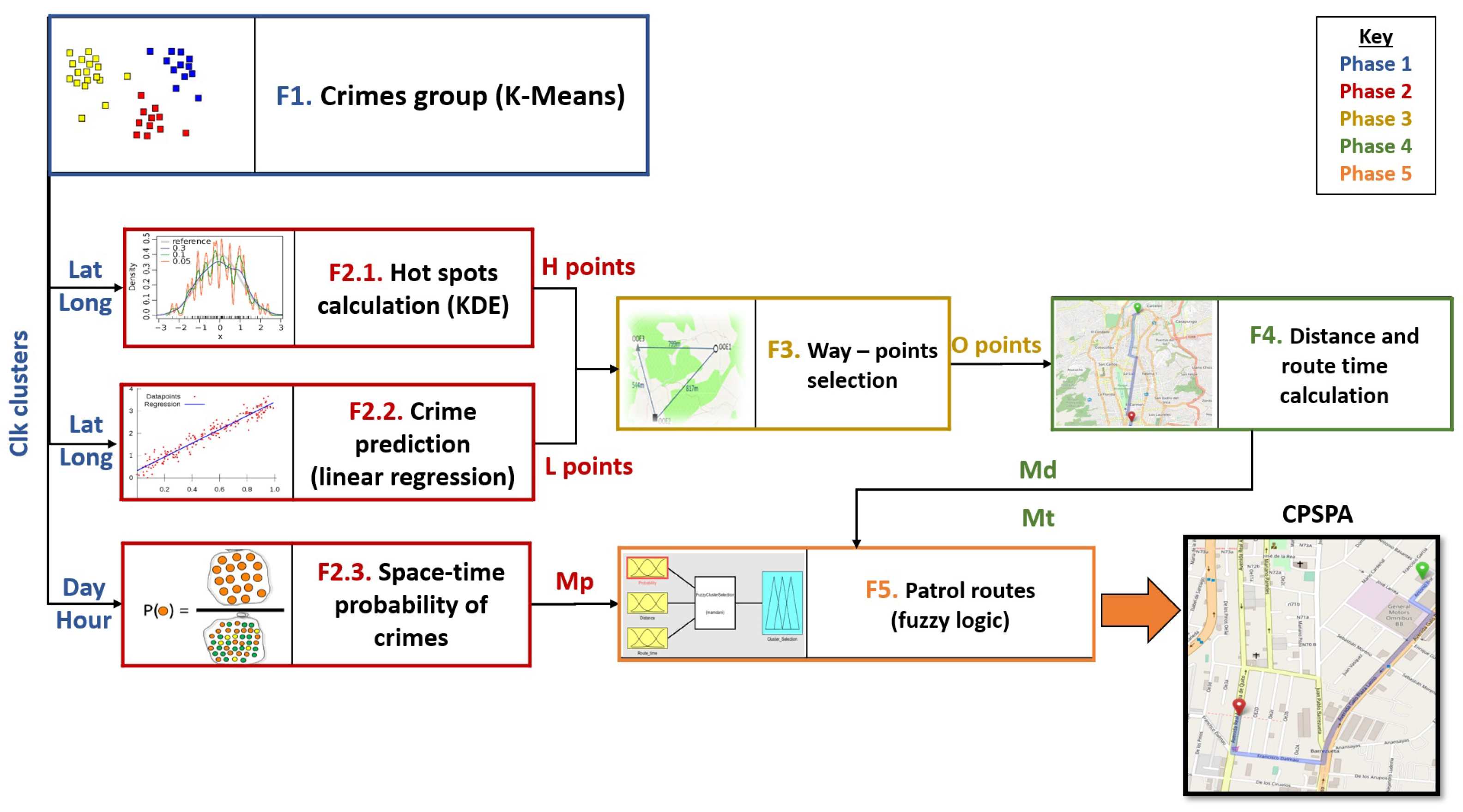
The CPSPA algorithm is structured in five phases (Figure 5). Along them, different ML techniques and statistical analysis are applied depending on the objective, to finally determine the prediction of possible crimes and propose the optimal route that a police officer should take during a surveillance turn.

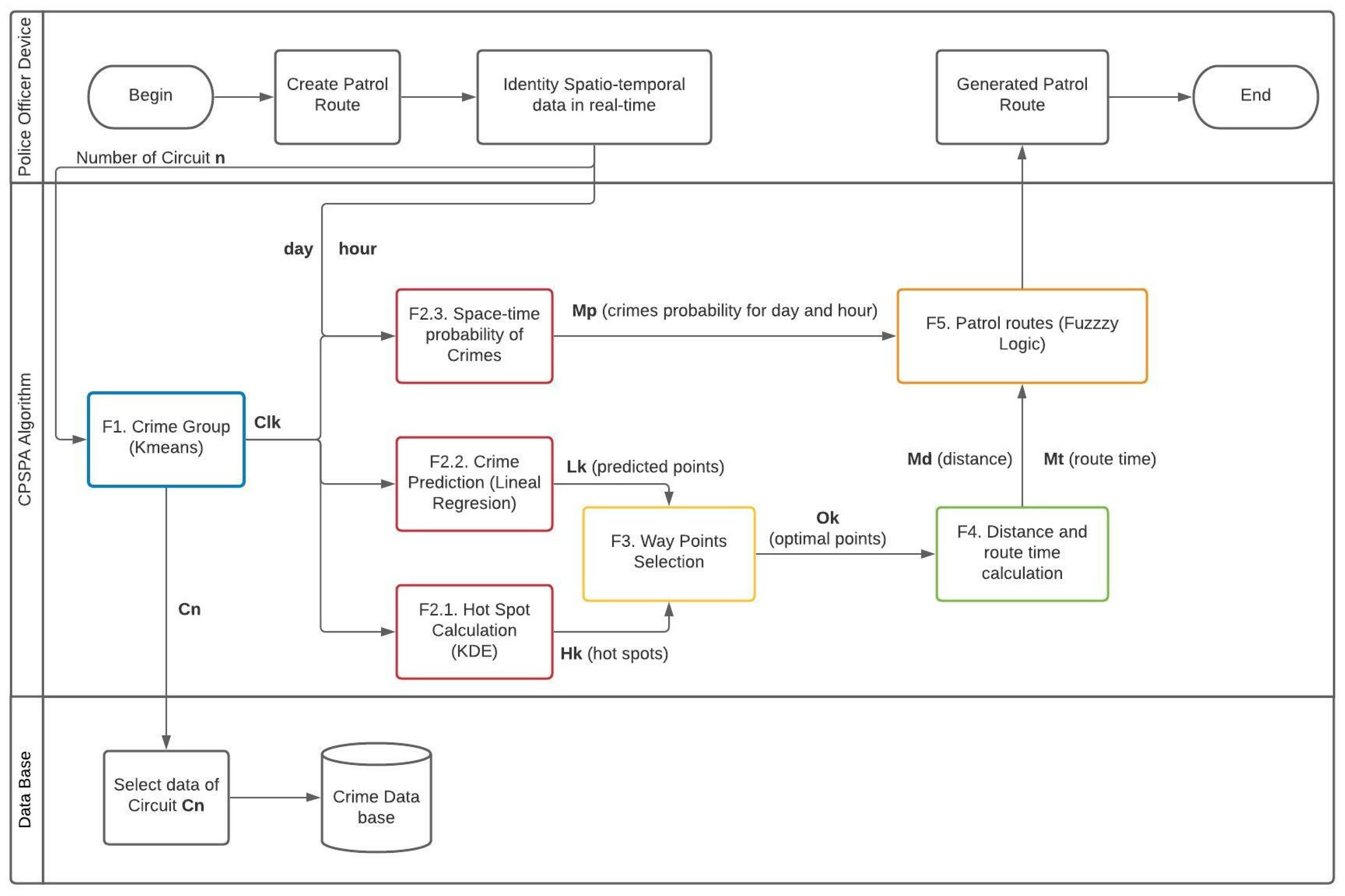
To clarify the algorithm, although the different steps are going to be described in detaile in the next sections, Figure 6 shows the activity UML diagrams. It shows the interaction among the Police Officer Device, the CPSPA algorithm and the database. The sequence of actions carried out to patrol the most conflictive points for each surveillance shift is shown. This diagram has as inputs the circuit that is being patrolled, $C_n$, and day and time of the patrol. The output is the police patrol route obtained, that consists of a starting point, some way-points along the route, and the final point. This diagram includes all the phases of the CPSPA algorithm.

In addition, Figure 7 presents the sequence diagram of the operation of the CPSPA algorithm. It is possible to see how some of the activities can be carried out in parallel.

The selected initial conditions of the experiments, after data analysis (Section 3), are the circuits $C_{n=2}$, $C_{n=10}$ y $C_{n=10}$, all of them belonging to $D_{05}$ district, due to the high number of reported crime records. The Matlab 2021a software and the Nvidia Geforce GTX 1050 GPU with frame buffer: 4 GB GDDR5, 7 Gbps memory speed have been used for the simulation. The phases of the algorithm are described below.

5.1. Phase 1. Crime Grouping from Criminal Database

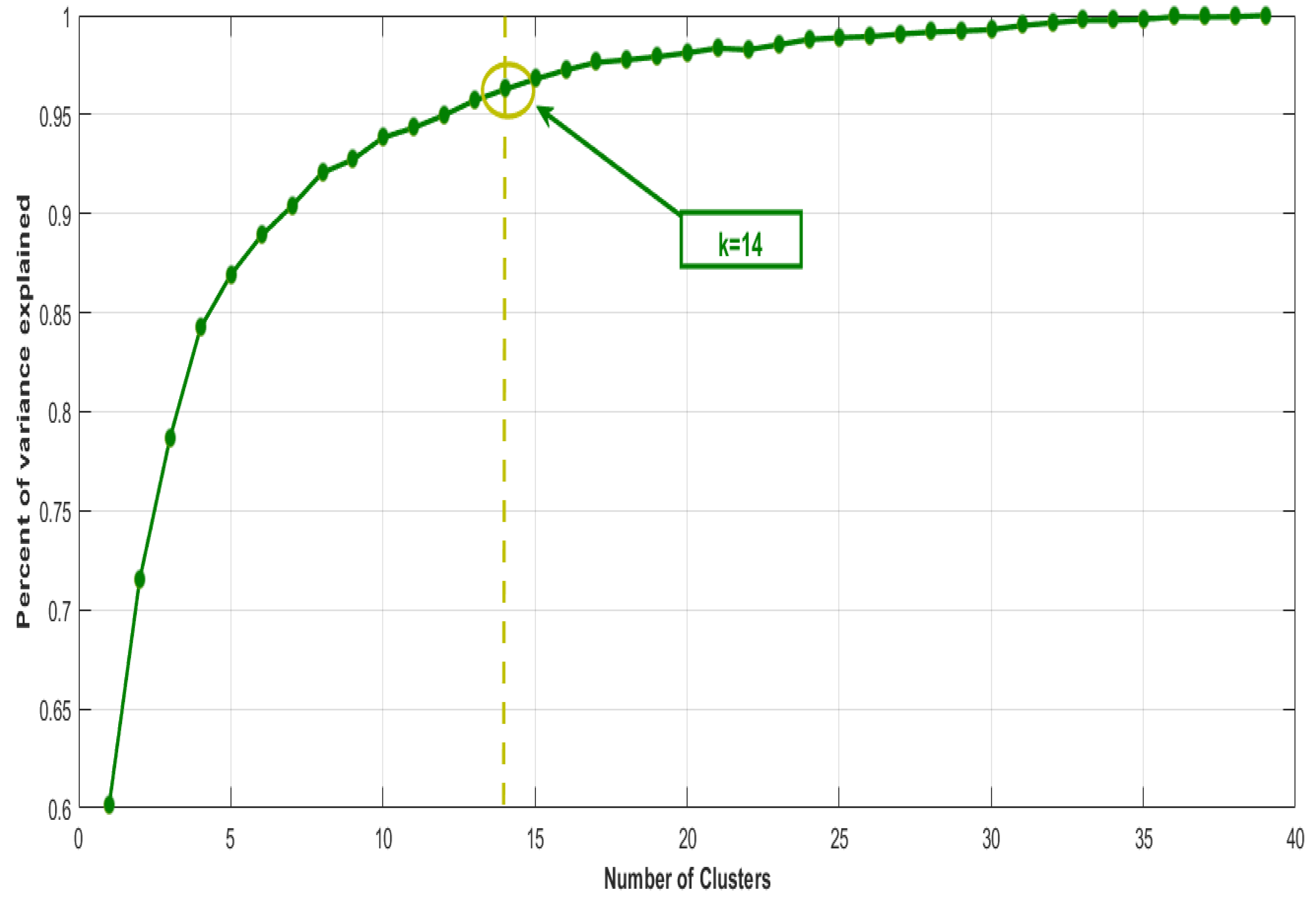
In this phase (see Figure 5), the crimes of a $C_n$ circuit are grouped using the k-means algorithm. As it is an unsupervised clustering, the optimal number of clusters k is obtained with the Elbow method. The objective is to determine the most conflicting areas, $C{l}_k$ (clusters), in circuit $C_n$, to analyze crimes in more detail. A number of crimes r has been reported in the area that represents each cluster, that is, $d{e}_{C{l}_k}=\{d{e}_1,d{e}_2,d{e}_3,...,d{e}_r\}$. 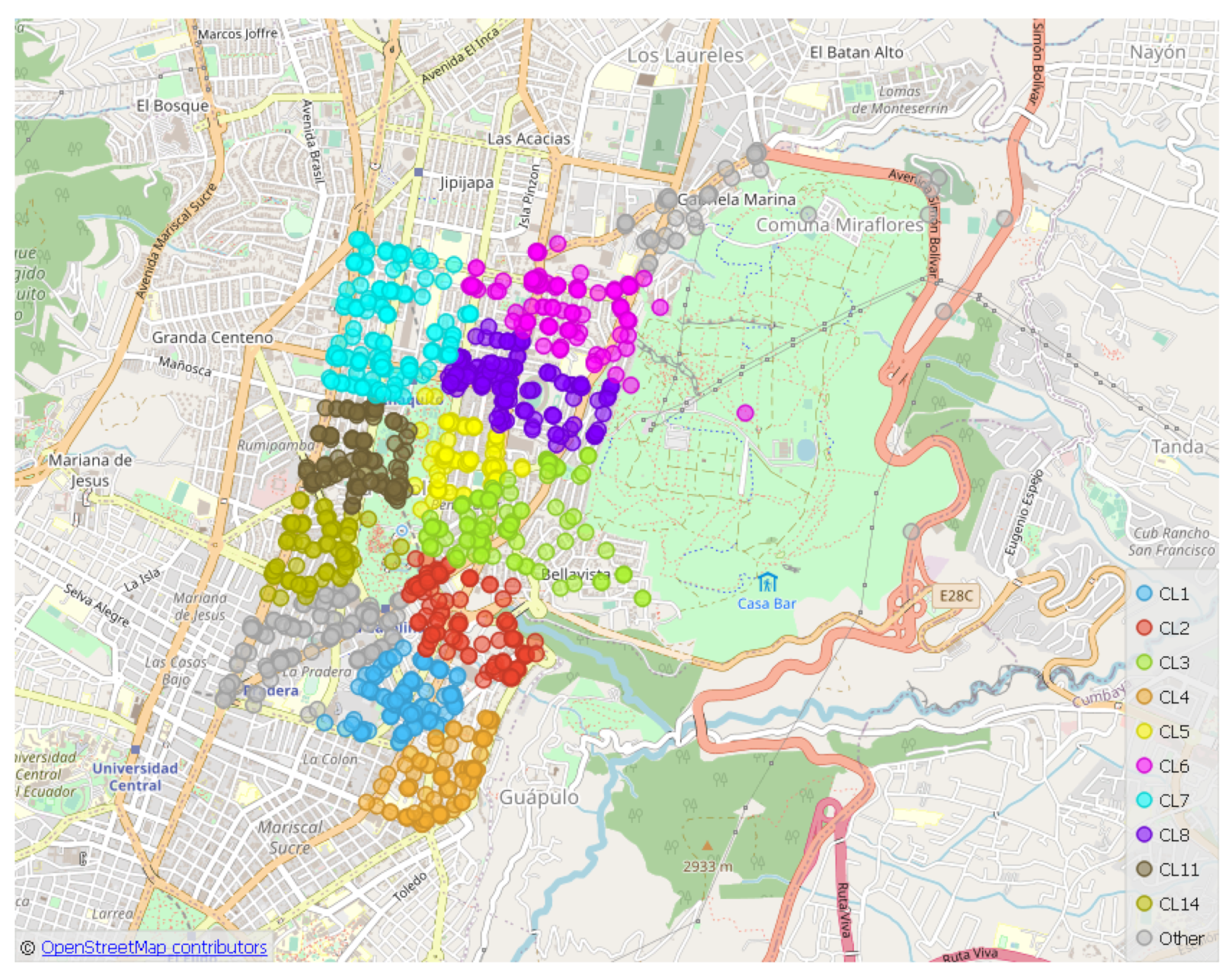As an example: within district $D_{05}$ the circuit $C_{10}$ is analyzed, which has 1539 crimes, $de$, reported in 2017. The k-means algorithm is applied with the Elbow method, and the optimal number of clusters is determined, $k=14$ (Figure 8). In Figure 9, the k groups are represented for the $C_{10}$ circuit in OpenStreetMap.

The k-means method has been applied because it is a well-know algorithtm that suits the objective of this phase, which is to determine crime concentration zones, including several geographic areas, as sub-circuits, although any other grouping algorithm may be used. Besides, the outcomes of its application gave similar results to those of the expert. Finally, k-means is simple, easy and quick to use and implement in an online real system.

5.2. Phase 2. Calculation of Hotspots, Prediction, and Probability of Crimes

At this stage, the spatial information, latitude, and longitude, is used to calculate hotspots (Phase 2.1, Section 5.2.1) and perform crime prediction in each cluster, (Phase 2.2, Section 5.2.2). With the temporal information, the spatial-temporal distribution of crimes is calculated (Phase 2.3, Section 5.2.3) (see Figure 5).

5.2.1. Phase 2.1. Calculation of Hotspots by Applying KDE

Hotspots are crime concentration points, defined as $H=\{H_1,H_2,H_3,...,H_k\}$. That is, a hotspot is calculated for each cluster determined in Phase 1, Section 5.1. KDE Equation (3) is applied to the spatial data of each crime, $lat,long$, to obtain the hotspot vector H.

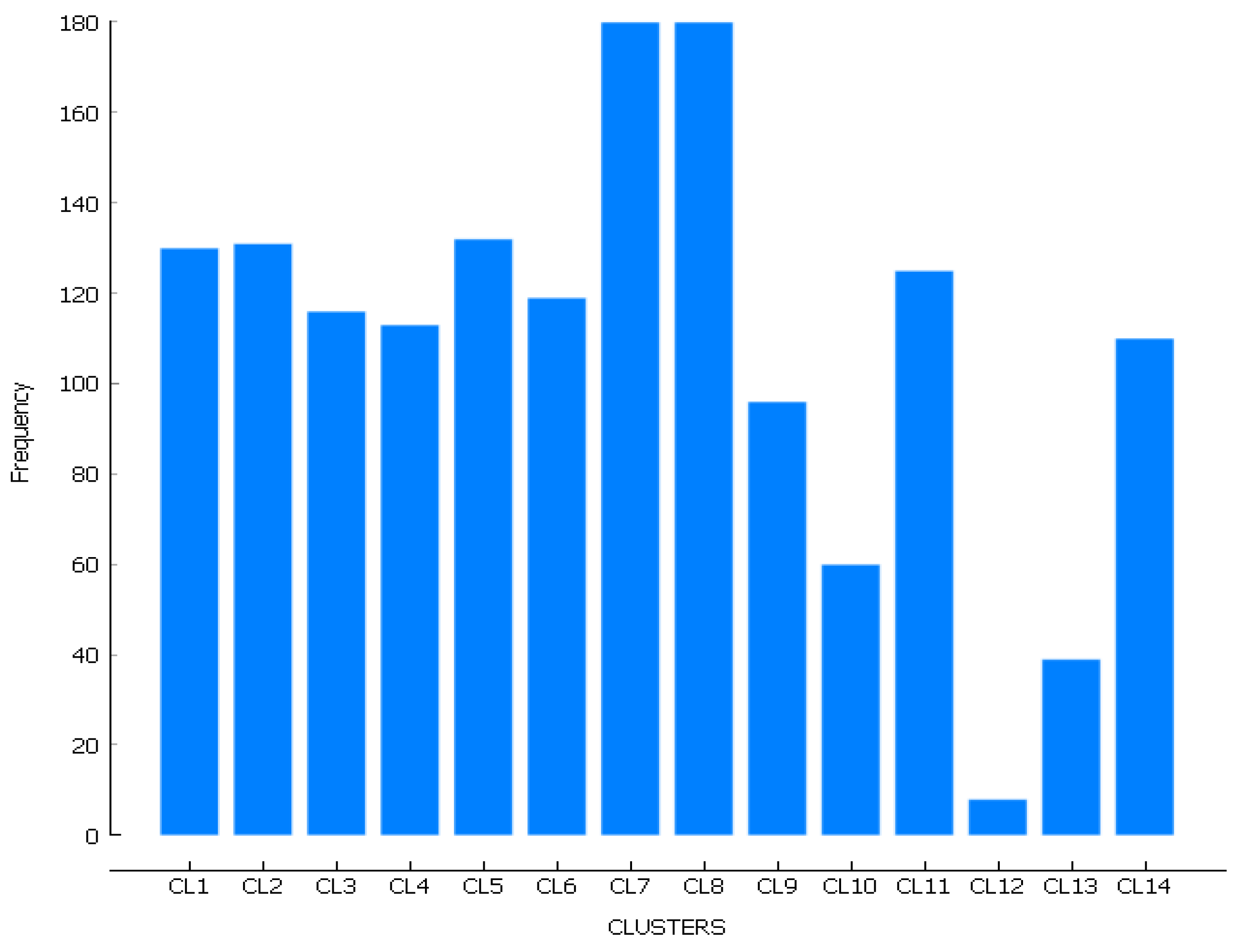
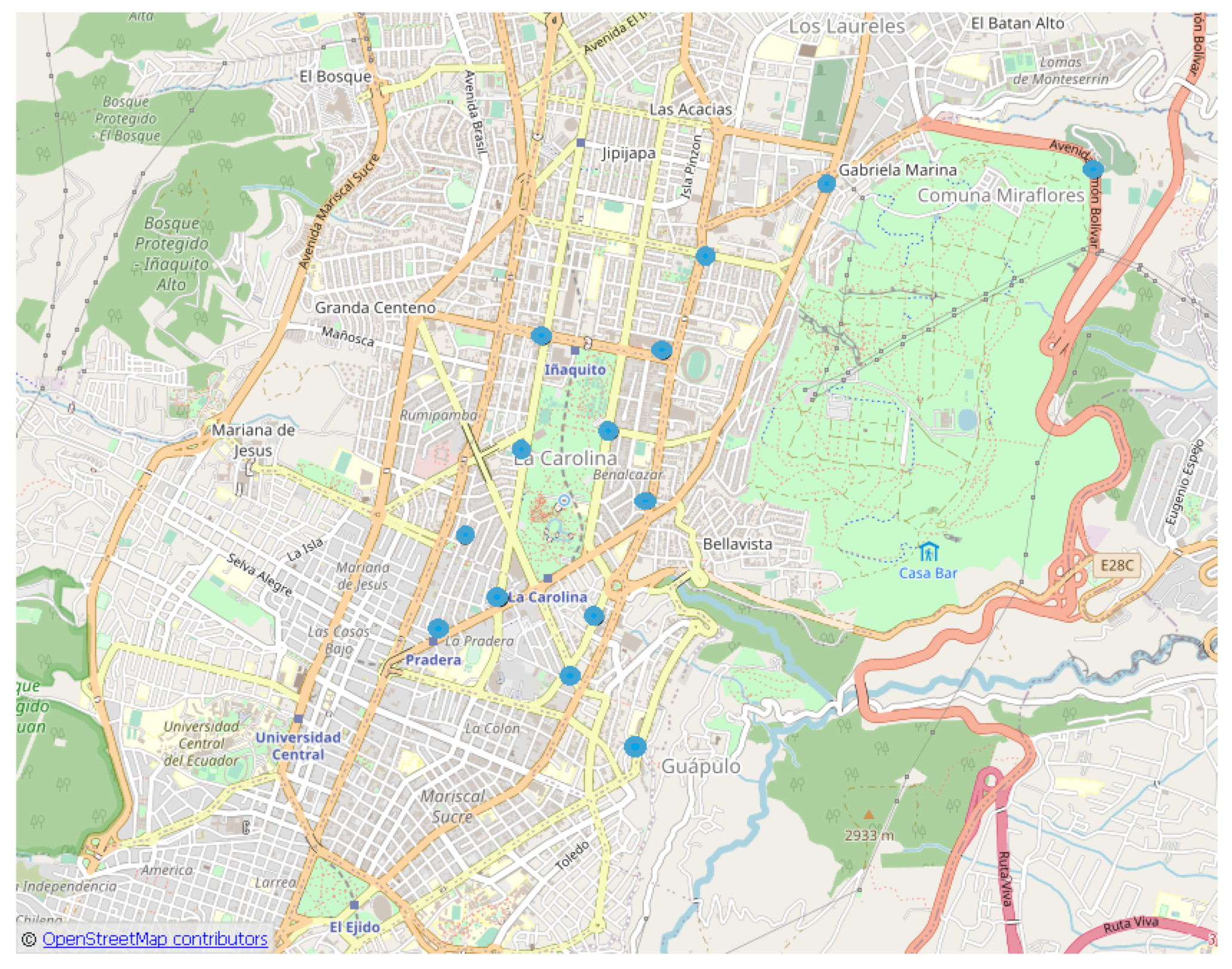
In the example, each of the 14 clusters in $C_{05}$ circuit has several records (offenses), with a maximum of $r=180$ in clusters $C{l}_7$ and $C{l}_8$, and a minimum of $r=8$ in $C{l}_{12}$ (Figure 10). H points with the highest concentration (hotspots) of crimes that result from applying KDE are represented by the blue circles in Figure 11, one for each cluster, for the $C_{05}$ circuit.

The light blue circles in Figure 11 represent the position of the point with the highest crime concentration within each cluster.

5.2.2. Phase 2.2. Crime Point Prediction via Linear Regression

In Phase 2.2 (see Figure 5), linear regression is used to obtaine models that can be used for crime prediction. To do so, Equation (4) is applied to the crime records of each cluster $C{l}_k$. Thus, the L points where the concentration of crimes may be higher, $L=\{L_1,L_2,L_3,...,L_k\}$, $k=14$, are obtained.

The crimes were ordered chronologically, $de=\{mt,dy,hr\}$. Then, with the spatial information, two linear functions are generated for each cluster, that is, $f_{lat}(C{l}_k=\left\{lat\right\})$ and $f_{long}(C{l}_k=\left\{long\right\})$. That is, $L_k=\{lat,long\}$ predicts the future crime concentration point of the k cluster. Those two linear functions have been obtained for each of the 14 clusters $C{l}_k$ of the $C_{05}$ circuit.

For instance, for cluster $C{l}_2$ the equations obtained when applying the linear regression are: $f_{lat}=-3.187\times {10}^{-6}x-0.1912$ for latitute and $f_{long}=-5.199\times {10}^{-6}x-78.48$ for longitude. The $R^2$ obtained was $0.48$ and the resulted regresion point was $L_k=(-0.194375911761479,$$-78.4791191630853)$. The R-squared values were between $0.40$ and $0.53$ for the 14 clusters.

5.2.3. Phase 2.3. Space-Time Probability of Crimes

In this last step of Phase 2 (see Figure 5), a crime probability matrix $Mp$ is calculated for each $C{l}_k$ cluster for the days and hours of a patrol turn. The $Mp$ matrix has dimensions (row, column), where $row=nd\times nh\times k$, $column=nc$, $nd=$ number of days, $nh=$ number of patrol hours, and $k=$ number of clusters. The four columns of $Mp$ matrix represent the day, time, cluster, and probability of crimes; hence, $nc=4$.

The $Mp$ matrix is obtained by applying Algorithm 1. The variables and symbols used are as follows. The datasets are divided into three surveillance turns, as carried out by the Ecuadorian National Police for their patrols. Turn 1 covers the schedule from 00:00 to 7:59, turn 2 runs from 8:00 a.m. to 3:59 p.m., and turn 3 runs from 4:00 p.m. to 11:59 p.m.

The total amount of crime on a circuit is $tde$. Each offense is assigned to a day ($dy$), hour ($hr$), and cluster $C{l}_k$. The crimes on a given day and time are $totCrCl$. The number of crimes per day, hour, and cluster is $repCr$. Equation (5) is applied to calculate the probability that a crime will take place that day, time, and in the spatial location of a given cluster.

$$P(d{e}_j=(dy,hr,C{l}_k))=\frac{repCr}{totCrCl}$$

(5)

That is, the quotient between all the crimes in a cluster and the total number of crimes in the circuit. For example, the probability of a crime on a Monday ($dy=1$) at 6:00 p.m. ($hr=18$) in cluster 3 ($C{l}_{k=13}$) would be: $P(de=(dy=1,hr=18,C{l}_{k=13}))=5/24=0.2083$.

The Mp matrix has a dimension of 588 × 4. An example of a row is: $[d{y}_i,h{r}_j,C{l}_k,P(d{e}_j=(dy,hr,C{l}_k))]=[2,19,3,015]$.

5.3. Phase 3. Selection of Surveillance Points

In this Phase 3 (see Figure 5), the information obtained in previous subsections will be integrated to determine the way points that the patrol route must follow. First, hotspots $H_k$ are obtained in each cluster, which may or may not coincide with the prediction points of maximum crime $L_k$. The distance between them is calculated so that if they are very distant from each other, a midpoint will be obtained. If they are very close to each other, the hotspot $H_k$ will be selected.

Algorithm 1 Obtaining the Crime Probability Matrix $Mp$ in a Cluster.

Inputs: $h{r}_{start}$ %turn start time% $h{r}_{end}$ %turn end time%  Output: $Mp\left[\right]$ %Crime Probability Matrix%  for $dy=1$ to $nd$ do   for $hr=h{r}_{start}$ to $h{r}_{end}$ do    for $C{l}_i$, $i\leftarrow 1$ to k do     for $j\leftarrow 1$ to $tde$ do      if ($d{e}_j\left(dy\right)==day$ AND $d{e}_j\left(hr\right)==hour)$ then       $totCrCl+1$      end if      if ($d{e}_j\left(dy\right)==day$ AND $d{e}_j\left(hr\right)==hour$ AND $d{e}_j\left(Cl\right)==i$) then       $repCr+1$      end if     end for     $row+1$;     $Mp(row,column=1)\leftarrow dy$;     $Mp(row,column=2)\leftarrow hr$;     $Mp(row,column=3)\leftarrow Cl$;     $Mp(row,column=4)\leftarrow repCr/\left(totCrCl\right)$;    end for   end for  end for

The Euclidean distance between $H_k=\{lat,long\}$ and $L_k=\{lat,long\}$, is applied.

$$d_E(H_k,L_k)=\sqrt{{(la{t}_H-la{t}_L)}^2+{(lon{g}_H-lon{g}_L)}^2}$$

(6)

The distance must meet the following conditions to determine the waypoints:

$$O_k=\left\{\begin{array}{cc}\hfill d_E,& d_E=0⟶O_k=L_k\hfill \\ \hfill d_E,& d_E>ϵ⟶O_k=H_k\hfill \\ \hfill d_E,& ϵ>d_E>0⟶O_k=P_{mean}=(\frac{la{t}_H-la{t}_L}{2},\frac{lon{g}_H-lon{g}_L}{2})\hfill \end{array}\right\}$$

where $ϵ$ is a constant (threshold) that limits the maximum distance between the hot spot $H_k$ and the predicted point $L_k$, defined as $ϵ=0.01$ (1 km). With this expression, a vector is obtained with the way-points $O_k$, which the patrol route should go through.

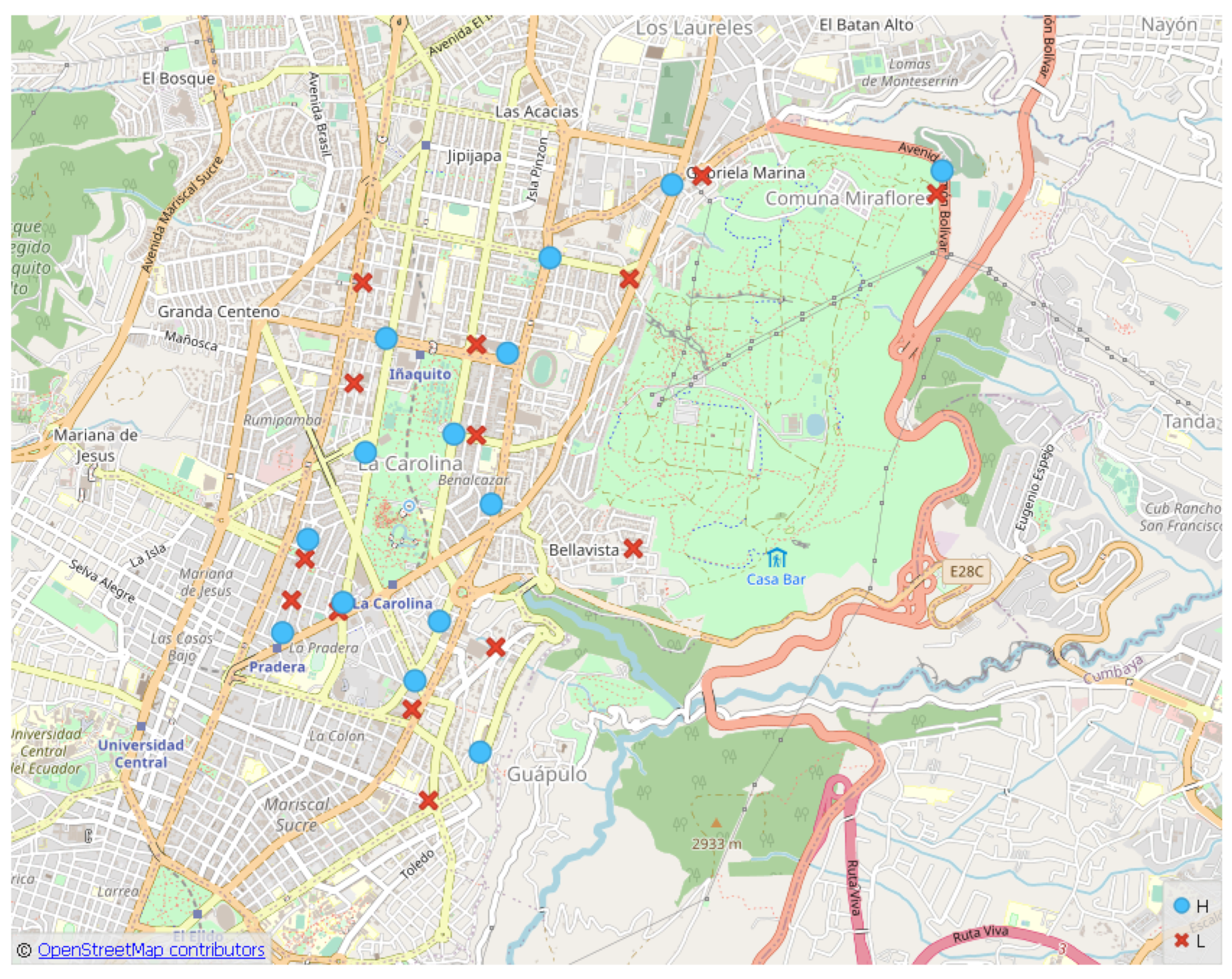
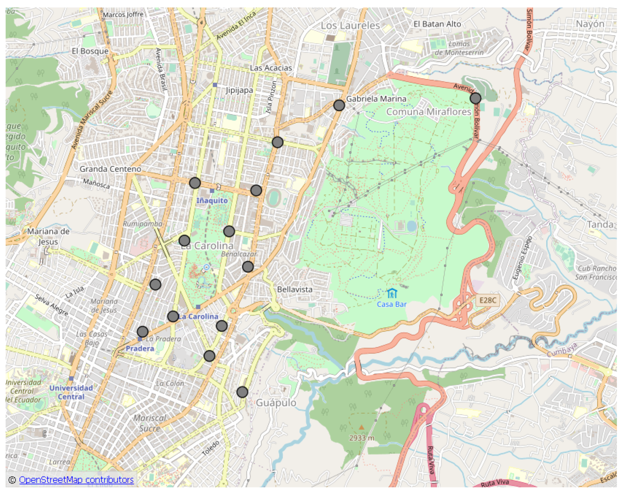
In Figure 12, the points $H_k$(light blue circles) and $L_k$ (x red markers) are shown. In Figure 13, the points $O_k$ (gray circles) resulting from the selection of points for the routes of the $C_{10}$ circuit are presented. Each cluster has one point.

As an example of this phase, in cluster $C{l}_1$, the hotspot is $H_1$ ($lat=-0.196$,$long=-78.483$), and the prediction shows $L_1$ ($lat=-0.198$,$long=-78.484$), where $d_E=0.0017<ϵ$. Hence, $P_{mean}$ is calculated as follows:

$$P_{mean}=(\frac{(la{t}_{H_1}=-0.196)-(la{t}_{L_1}=-0.198)}{2},(\frac{(lon{g}_{H_1}=-78.483)-(lon{g}_{L_1}=-78.484)}{2}).$$

The resulting way-point $O_1$ has the coordinates $(-0.196,-78.483)$.

%vspace-6pt

5.4. Phase 4. Distances and Route Time Calculation with OpenStreetMap API

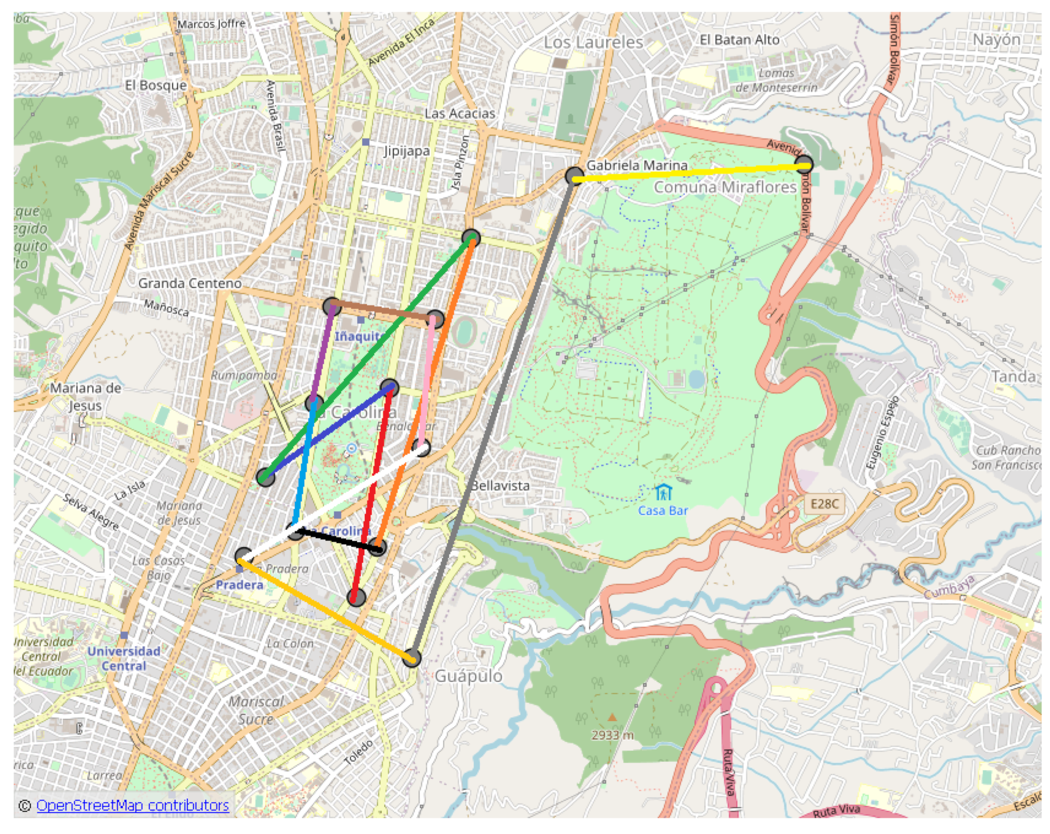
The distance and driving time between the way points must be determined to find the best patrol route. In a city, a distance may be small but it may take a long time to travel due to the conditions of the road or due to traffic at certain times. To obtain realistic values, the distance and travel time between the $O_k$ way points are obtained with the API (Application Programming Interface) of the OpenStreetMap application. The result is represented in the square matrices $M{d}_{k,k}$ (distance in km) and $M{t}_{k,k}$ (time in minutes) from the initial point $O_i$ to the end point $O_j$.

The distanceAPI (distance of travel) function is applied to obtain the elements, $dAp{i}_{i,j}=distanceAPI(O_i,O_j)$, of the matrix $M{d}_{k,k}$.

$$M{d}_{k,k}=\left[\begin{array}{cccc}dAp{i}_{1,1}& dAp{i}_{1,2}& ...& dAp{i}_{1,j}\\ dAp{i}_{1,2}& dAp{i}_{2,2}& ...& dAp{i}_{2,j}\\ ...& ...& ...& ...\\ dAp{i}_{i,1}& dAp{i}_{i,2}& ...& dAp{i}_{i,j}\end{array}\right]$$

In our case, the matrix $M{d}_{14,14}$, has the results of the distance API($O_i$,$O_j$) functions, where, for example, the distance between $O_1(-0.196,-78.483)$ and $O_2(-0.192,-78.482)$ is $dAp{i}_{1,2}=0.85$.

$$M{d}_{k,k}=\left[\begin{array}{ccccc}dAp{i}_{1,1}=0& dAp{i}_{1,2}=0.85& dAp{i}_{1,3}=2.8& ...& dAp{i}_{1,14}=1.8\\ dAp{i}_{2,1}=1.4& dAp{i}_{2,2}=0& dAp{i}_{2,3}=1.9& ...& dAp{i}_{2,14}=1.5\\ dAp{i}_{3,1}=2.3& dAp{i}_{3,2}=1.2& dAp{i}_{3,3}=0& ...& dAp{i}_{3,14}=1.7\\ ...& ...& ...& ...& ...\\ dAp{i}_{14,1}=1.5& dAp{i}_{14,2}=1.7& dAp{i}_{14,3}=2.4& ...& dAp{i}_{14,14}=0\end{array}\right]$$

In the same way, the OpenStreetMap timeAPI (travel time) function is used to calculate the route time, $tAp{i}_{i,j}=timeAPI(O_i,O_j)$, which are the elements of matrix $M{t}_{k,k}$.

$$M{t}_{k,k}=\left[\begin{array}{cccc}tAp{i}_{1,1}& tAp{i}_{1,2}& ...& tAp{i}_{1,j}\\ tAp{i}_{1,2}& tAp{i}_{2,2}& ...& tAp{i}_{2,j}\\ ...& ...& ...& ...\\ tAp{i}_{i,1}& tAp{i}_{i,2}& ...& tAp{i}_{i,j}\end{array}\right]$$

For instance, in the matrix $M{t}_{14,14}$, timeAPI($O_i$,$O_j$) between the points $O_1(-0.196,-78.483)$ and $O_2(-0.192,-78.482)$ is $tAp{i}_{1,2}=4$.

$$M{d}_{k,k}=\left[\begin{array}{ccccc}tAp{i}_{1,1}=0& tAp{i}_{1,2}=4& tAp{i}_{1,3}=9& ...& tAp{i}_{1,14}=8\\ tAp{i}_{2,1}=5& tAp{i}_{2,2}=0& tAp{i}_{2,3}=6& ...& tAp{i}_{2,14}=6\\ tAp{i}_{3,1}=11& tAp{i}_{3,2}=8& tAp{i}_{3,3}=0& ...& tAp{i}_{3,14}=9\\ ...& ...& ...& ...& ...\\ tAp{i}_{14,1}=5& tAp{i}_{14,2}=7& tAp{i}_{14,3}=10& ...& tAp{i}_{14,14}=0\end{array}\right]$$

5.5. Phase 5. Application of Fuzzy Logic to Determine Patrol Routes

Finally, once the way-points $O_k$ of route and the information on the probability of crimes and proximity, both in length (distance) and route time, have been determined, the route to be taken must be decided. A fuzzy decision-making system (FDSS) that uses probability matrices, $Mp$, distances, $Md$, and route times, $Mt$, has been designed.

Given that it is possible to obtain several solutions that can be equally valid, fuzzy logic is used because it allows the representation of variables including the uncertainty associated with route times, probability, and so on. The fuzzy decision-making system has three input variables, normalized to $[0,1]$:

1.

Route distance - $R{d}_k$: distance from the initial point $Pi$ to the final point $Pf$. This variable has been assigned three fuzzy sets with triangular membership functions: near (0 to $0.4$), middle ($0.1$ to $0.9$), and far ($0.6$ to $1.0$). They correspond to the information in matrix $Md$, with $R{d}_k=Md(Pi,Pf)$.

2.

Route time - $R{t}_k$: route time from the initial point $Pi$ to the final point $Pf$. The same fuzzy sets have been assigned as for the previous variable. Travel times are found in matrix $Mt$, with $R{t}_k=Mt(Pi,Pf)$.

3.

Crime spot probability - $P{\left(CS\right)}_k$: the probability of crimes at the destination point $Pf$, on a given day $dy$ and hour $hr$. Three fuzzy sets with triangular membership functions have been assigned to this variable: low (0 to $0.4$), medium ($0.1$ to $0.9$), and high ($0.6$ to $1.0$). These probabilities are identified in matrix $Mp$.

The output variable is called point selection ($PS$), which determines if a way-point $O_k$ is selected as the next way point of the route. It outputs two fuzzy singletons: selected and unselected.

The fuzzy decision-making system rules are, for instance: If $P\left(CS\right)$ is High and $Rd$ is Middle and $Rt$ is Near, then Point Selection is NOT SELECTED. The route implementation algorithm after applying the fuzzy decision system is shown in Algorithm 2.

Algorithm 2 Patrol route Implementation.

Inputs: $O_k$ % Way points $Mp$ % probability matrix $Md$ % distance matrix $Mt$ % route times matrix  Output: $rPoint$ % order of points of the patrol route  for $i=1$ to k do   $Pi=O_i$;   for $f=1\leftarrow k$ do   $Pf=O_j$   $Rd=Md(Pi,Pf)$;   $Rt=Mt(Pi,Pf)$;   $P\left(Cs\right)=Mp\left(P(de=(dy=d{y}_{start},hr=h{r}_{start},C{l}_{k=f}))\right)$;   $rPoint=FDSS\left(P\right(Cs),Rd,Rt)$;   if $rPoint$ == SELECTED then   Carry out patrol of $O_i$ a $O_j$;   $d{y}_{start}+Rt$;   end if  end for end for

6. Results and Discussion

Numerous simulation experiments have been carried out with criminal records of the first (1729 reported crimes) and second (1498 reported crimes) semesters of 2017. The route algorithm is applied to circuits with a high incidence of crimes, specifically $C_{02}$, $C_{06}$ y $C_{10}$. These simulations will be compared with those carried out by a citizen security expert from the national police of Ecuador.

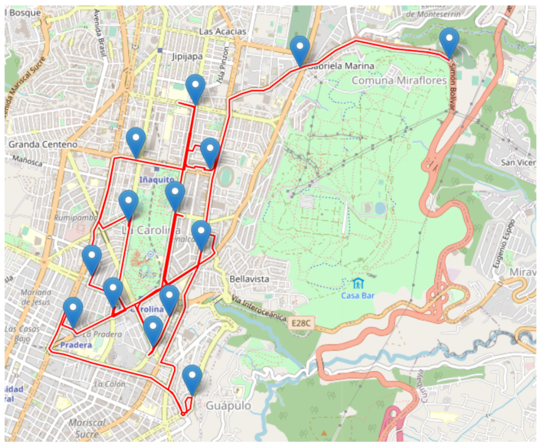
The results of the application of the decision made for the patrol route for a specific case are shown in Figure 14 and Figure 15 and

Table 2. Patrol Route Selection Data with CPSPA Algorithm.

Route	Color	Probability	Distance (km)	Time (min)	Hour
Route 1	Red	0.05	2.5	9	18:09
Route 2	Blue	0.14	2.3	12	18:21
Route 3	Green	0.06	2.0	12	18:33
Route 4	Orange	0.02	1.4	13	18:46
Route 5	Black	0.09	1.4	5	18:51
Route 6	Light blue	0.11	0.9	3	18:54
Route 7	Purple	0.07	1.8	4	18:58
Route 8	Brown	0.08	2.4	6	19:04
Route 9	Pink	0.03	2.7	9	19:13
Route 10	White	0.10	1.7	8	19:21
Route 11	Dark Yellow	0.04	2.8	9	19:32
Route 12	Gray	0.13	6.1	10	19:42
Route 13	Yellow	0.12	2.6	11	19:53
Total			30.6	111

, where the probabilities (Equation (5)), distances, route time, and time of the patrol between each of the points (blue points Figure 15) are listed. In this specific example, the patrol day is $dy=6$ (Saturday), the start time is $h{r}_{start}=18$, and the patrol starting point is $O_{k=1}$. The obtained patrol route is $30.6$ km.

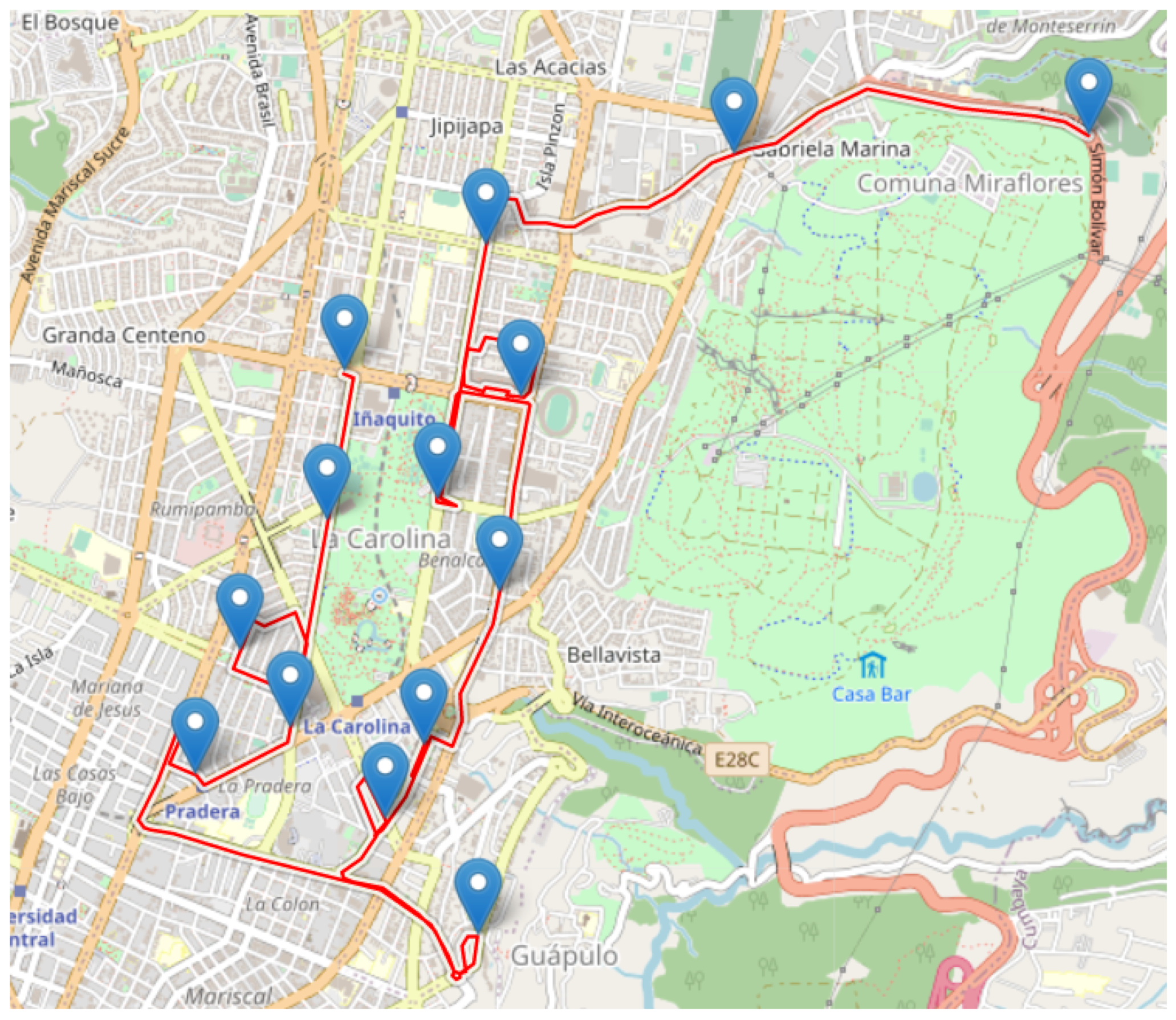
The results obtained by the security expert (

Table 3. Patrol route selection data from expert decision.

Route	Color	Probability	Distance (km)	Time (min)	Hour
Route 1	Light blue	0.0004	0.75	8	18h08${}^{\prime }$
Route 2	Red	0.0061	1.3	14	18h22${}^{\prime }$
Route 3	Yellow	0.0014	1.0	9	18h31${}^{\prime }$
Route 4	Orange	0.0026	0.6	3	18h34${}^{\prime }$
Route 5	Blue	0.0039	3.6	22	18h56${}^{\prime }$
Route 6	Purple	0.0018	2.3	12	19h08${}^{\prime }$
Route 7	Gray	0.0060	1.8	14	19h22${}^{\prime }$
Route 8	White	0.0009	1.5	16	19h38${}^{\prime }$
Route 9	Green	0.0079	2.2	20	19h58${}^{\prime }$
Route 10	Pink	0.0081	1.8	16	20h14${}^{\prime }$
Route 11	Brown	0.0086	1.0	9	20h25${}^{\prime }$
Route 12	Black	0.0093	1.7	12	20h37${}^{\prime }$
Route 13	Dark Yellow	0.0097	3.8	20	20h57${}^{\prime }$
Total			21.65	175

, Figure 16 and Figure 17) showed lower probability rate for each generated route. The expert has estimated the probability of the routes using date, hour and a specific geographical area. The distance obtained by the expert was 21.65 km, smaller in comparison to the one obtained by the proposed algorithm, 30.6 km. The total time patrolling route was 175 min, that is, slower than the CPSPA algorithm, with 111 min. In general, the results show that the CPSPA algorithm works with the most relevant variables and finds valid routes that may help find new routes with some advantages.

In addition, as previously mentioned, the period of a semester (6 months) has been proved to have enough information of crimes to deal with, but still it may be not large enough for a more complete analysis of the data. Hence, to further test the algorithm, it has been applied to the second half of 2017 set of data.

Table 4. Resultsin circuits $C_{02}$, $C_{06}$, y $C_{10}$ with data from the second semester of 2017.

Datasets	Records	${\mathit{O}}_{\mathit{k}}$	Distance (km)	Accuracy	Time (min)	Processing Time (s)
$C_{02}$- Turn 1	105	8	34.70	85.01	164	226.919
$C_{02}$- Turn 2	157	10	35.90	81.03	172	273.192
$C_{02}$- Turn 3	295	13	39.60	79.78	197	292.792
$C_{06}$- Turn 1	37	6	28.50	77.52	101	187.984
$C_{06}$- Turn 2	92	7	30.10	77.48	114	194.682
$C_{06}$- Turn 3	103	9	33.00	82.39	139	226.281
$C_{10}$- Turn 1	100	9	31.20	76.88	124	242.634
$C_{10}$- Turn 2	238	14	33.40	80.11	145	269.965
$C_{10}$- Turn 3	371	15	30.60	76.99	111	311.484
Total	1498	Average	33.00	79.69	140.77	247.32

shows data and results working with this new data set: the number of crimes broken down into patrol turns in the first column; the $H_k$ hotspots of the circuits that are then calculated, and the $L_i$ predictions obtained of where crimes will take place for each circuit (Phase 2.2). If the distance between them is smaller than 1 km, $L_i$ will be set as way point of the route $O_k$.

$$Accuracy=\frac{deP}{(deP+deN)}100\%$$

(7)

The results obtained regarding accuracy are quite similar to [7,35], proving that finding patterns and predicting future crimes with clustered crimes in space and time is possible. When the rest of the phases of the algorithm are applied, the way points of the patrol routes, $O_k$, are selected. The route distance, route time, and processing time of the proposed algorithm are then calculated (Table 4). For each circuit, between 8 and 15 crime concentration points have been identified, depending on the schedule in which the surveillance is carried out. This value depends on the result obtained with k-means and the Elbow method.

A direct relationship was found between the number of crimes reported and the number of surveillance points. The number of crimes in turns 1 and 2 is smaller than in turn 3.

As shown in Table 4, the time of the route in each circuit has an average of 140.77 min (2 h 34 min). As each turn is 8 h, the route takes 29.32% of the total shift time. Turns 2 and 3 require more time due to traffic. Furthermore, turn 3 has a higher number of crimes.

The distance of the route has an average of $33.00$ km, which is efficient for covering a geographical area of 36 km${}^2$, with approximately 11,000 inhabitants. It depends on the number of way points of the route. The patrol distance increases for turn 2 and is even greater for turn 3.

For this reason, we initially analyzed the temporal data window to work with, as shown in Section 4.1, with the primary objective of determining an optimal period and the necessary historical crime data so that the efficiency of the proposed algorithm is high while time processing is not so demanding. It is worth it to note that adding more data is not relevant to the goal of the algorithm, it could improve the precision a bit but increasing computional time.

Indeed, the average processing time of the algorithm has been calculated, it is 247.32 s. Phases 4 and 5 require more computational time due to the execution of the OpenStreetMap API and the making decision system. The API depends on the speed of the internet connection and the processor of the local computer. The decision-making system uses many resources to generate optimal routes, both for points with high probability and for proximity. As expected, the larger the amount of data, the longer the algorithm processing time.

Therefore, this proposed algorithm provides appropriate routes for all selected way-points in the order the fuzzy logic system determines. When compared with other routes designed by a security expert, results are similar in time and distance, though the proposed method tends to obtain quicker routes. The solutions have been projected on a map of the affected zones where the results have been verified, and the obtained routes are realistic. The analysis of results allows for testing the successful performance of this strategy.

7. Conclusions and Future Works

In this research, an algorithm for the detection of spatio-temporal sources of crime is proposed. The final goal is to design patrolling routes to optimize police resources, reduce crime time response and improve citizen security.

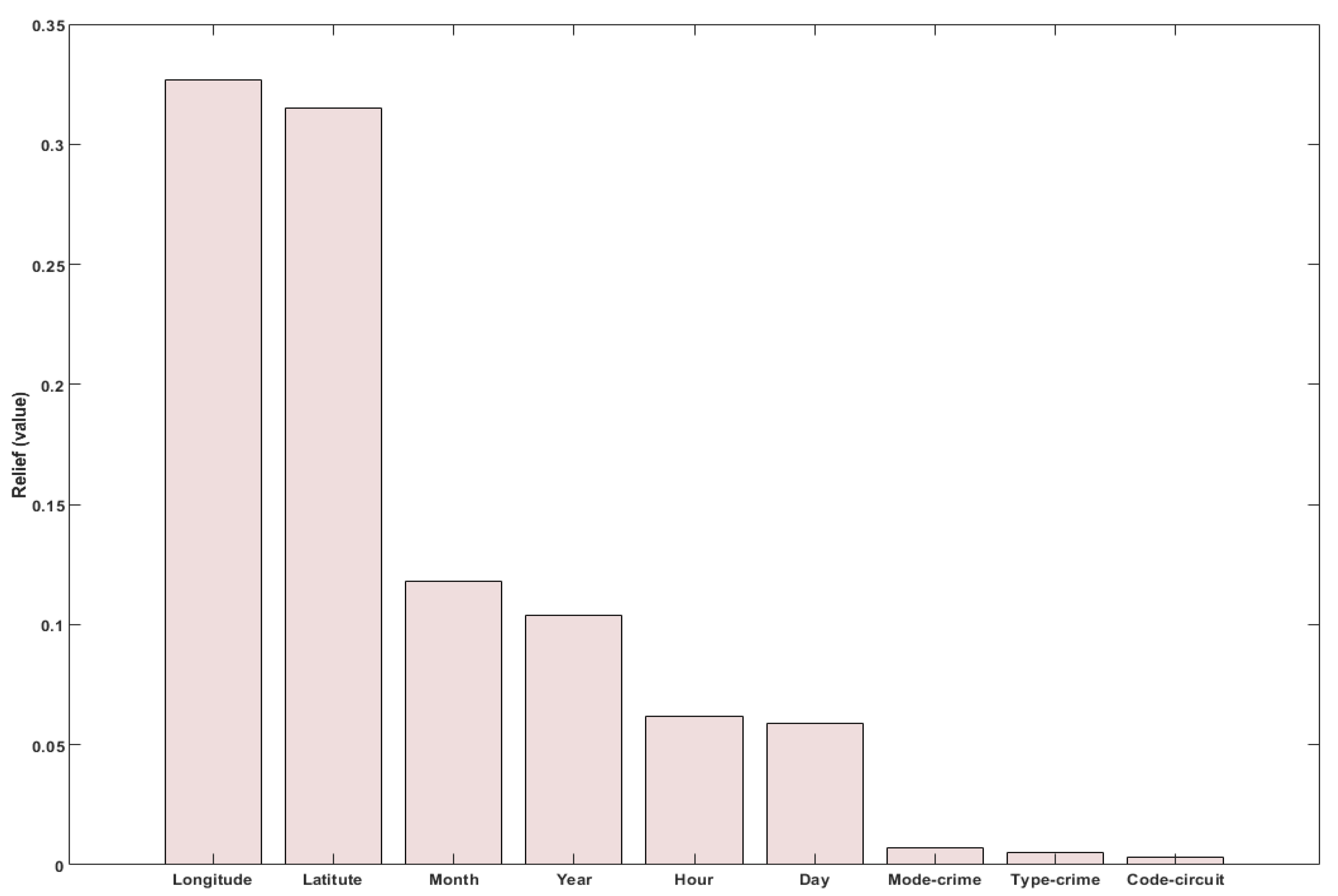
The algorithm consists of several phases and combines different artificial intelligent and ML techniques to deal with the available information. First, Relief and Information gain feature selection procedures are applied to obtain the relevant attributes. Hotspots with a high concentration of crime are identified by applying k-means clustering and KDE. A prediction of future crime points and the probability is obtained based on temporal information of the crimes. Spatial way points of routes are then calculated, and the real distance and travel time are computed with the OpenStreetMap API. Finally, a fuzzy inference system determines the order of the way-points in the route based on their probability, distance, and time.

The experimental evaluation was performed on a real crime dataset collected in Quito, Ecuador, in 2017. It allowed to conclude that this analysis makes it possible the use of information both in space and time of crimes committed in a region to determine policing more efficiently. Furthermore, the use of the OpenStreetMap API allows working with real measures and including traffic, giving more realistic solutions but at the cost of more computational time and resources.

The sequence of strategies applied along the procedure to determine the routes has been proved key to the succes of the algorithm. Besides, the hibridization of techniques has also been shown a must in order to address this type of complex problems. The complete development of the algorithm is presented, from the analysis and processing of the spatial and temporal information to the patrol routes generation. It allows to obtain automatically a patrolling route in a similar way to an expert.

To summarize, the main advantages of our proposal are that the route is automatically obtained, it is optimized in terms of time and distance, and the computational time is low. It is similar but more complete than the one proposed by the expert as it identifies the hot spots and future crime points, while the expert only works with hotspots in a specific area, so the available information is more limited. In addition, the routes obtained by the algorithm tend to be faster as they consider real time information of traffic.

For future research, we propose to study the generation of maps that incorporate temporal information of the surveillance zones to reduce the execution time of the algorithm and allows its use in real-time. It is also intended to continue analyzing the problem to improve patterns and prediction, incorporating information of the relationship between crimes and areas of population concentration, such as parks, shops, liquor stores, restaurants, and so on. From the algorithm point of view, other clustering techniques, such as Gaussian Mixture Models, Mean-Shift Clustering, and DBSCAN, may be tried to see how the tecnique chosed affects the results of the CPSPA algorithm.