Detection of River Floating Garbage Based on Improved YOLOv5

Abstract

The random dumping of garbage in rivers has led to the continuous deterioration of water quality and affected people’s living environment. The accuracy of detection of garbage floating in rivers is greatly affected by factors such as floating speed, night/daytime natural light, viewing angle and position, etc. This paper proposes a novel detection model, called YOLOv5_CBS, for the detection of garbage objects floating in rivers, based on improvements of the YOLOv5 model. Firstly, a coordinate attention (CA) mechanism is added to the original C3 module (without compressing the number of channels in the bottleneck), forming a new C3-CA-Uncompress Bottleneck (CCUB) module for improving the size of the receptive field and allowing the model to pay more attention to important parts of the processed images. Then, the Path Aggregation Network (PAN) in YOLOv5 is replaced with a Bidirectional Feature Pyramid Network (BiFPN), as proposed by other researchers, to enhance the depth of information mining and improve the feature extraction capability and detection performance of the model. In addition, the Complete Intersection over Union (CIoU) loss function, which was originally used in YOLOv5 for the calculation of location score of the compound loss, is replaced with the SCYLLA-IoU (SIoU) loss function, so as to speed up the model convergence and improve its regression precision. The results, obtained through experiments conducted on two datasets, demonstrate that the proposed YOLOv5_CBS model outperforms the original YOLOv5 model, along with three other state-of-the-art models (Faster R-CNN, YOLOv3, and YOLOv4), when used for river floating garbage objects detection, in terms of the recall, average precision, and F1 score achieved by reaching respective values of 0.885, 90.85%, and 0.8669 on the private dataset, and 0.865, 92.18%, and 0.9006 on the Flow-Img public dataset.

1. Introduction

With the rapid development of industry and agriculture, the living space for human beings is constantly expanding, the living standard is continuously improving, and the requirements for water quality consequently increase. However, due to soil erosion, massive dumping of garbage, and various other factors, the number of the aquatics is decreasing, the water is eutrophic, and the algae has overgrown in recent years, thus seriously affecting the quality of water. In the past, the main method used to control the quality of water was to manually check the river site conditions, and then apply a salvage procedure. To save unnecessary manpower, real-time monitoring of river dredging and blocking by means of patrolling or fixed cameras, or Unmanned Aerial Vehicles (UAVs) [1], has become a feasible and efficient way to detect floating garbage today.

As early as 2001, Viola and Jones proposed a real-time face detection model [2], working without any constraints. Later, Dalal and Triggs proposed the Histograms of Oriented Gradients (HOG) model [3], which made important improvements on both scale-invariant feature transforms and shaping contexts. In 2008, Felzenszwalb et al. proposed the Deformable Part Model (DPM) [4], which was later improved in [5,6], making it a leader in traditional object detection at that time. In 2014, Girshick et al. proposed the Region Convolutional Neural Network (R-CNN) model [7] with a cross-era significance. From then on, object detection began to develop rapidly. In the next year, He et al. proposed the Spatial Pyramid Pooling Network (SPPNet) [8], which introduced a spatial pyramid pooling layer to avoid repeated calculation of convolution features. In 2015, on the basis of R-CNN and SPPNet, Girshick proposed the Fast R-CNN model [9], with greatly improved detection speed and accuracy. In 2015, Ren et al. proposed the first end-to-end deep learning detector, Faster R-CNN [10], which broke through the speed bottleneck of Fast R-CNN, but was still suffering from computational redundancy in the subsequent detection phase. Therefore, later a variety of improved models were proposed, including R-FCN [11] and Light-head R-CNN [12]. In 2017, Lin et al. proposed the Feature Pyramid Network (FPN) [13] on the basis of Faster R-CNN, which has made great progress in detecting objects of various scales.

In 2015, Liu et al. proposed the Single Shot MultiBox Detector (SSD) [14], which introduced multi-reference and multi-resolution detection techniques with greatly improved detection accuracy. In the same year, Redmon et al. proposed the You Only Look Once (YOLO) model [15], which was the first single-stage detector in the era of deep learning. Later, Redmon et al. made a series of improvements in the first YOLO version and subsequently proposed new versions of it, i.e., YOLOv2 [16], YOLOv3 [17], followed by YOLOv4 [18,19], proposed by Bochkovskiy et al. In 2020, Ultralytics released YOLOv5 [20], which further improved the detection accuracy while maintaining high detection speed.

The objective of this paper is to come up with a novel model, called YOLOv5_CBS, based on YOLOv5 improvements, to achieve better river garbage detection, based on captured images. The main contributions of the paper can be summarized as follows:

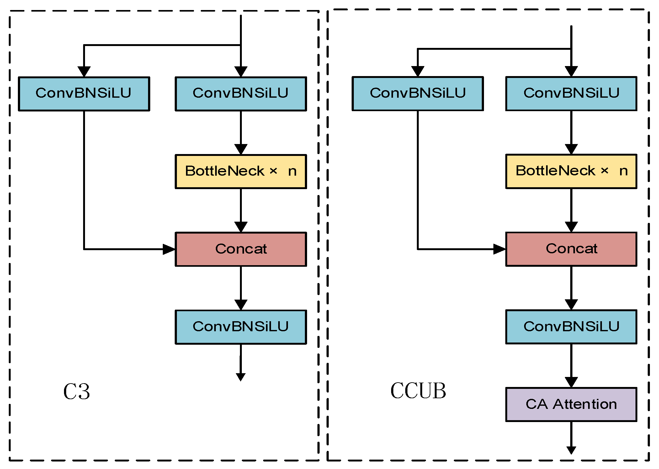
• Adding a coordinate attention (CA) [21] mechanism after the original C3 module of YOLOv5, as proposed in [22], but without compressing the number of channels in the bottleneck, which results in a new C3-CA-Uncompress Bottleneck (CCUB) module used for increasing the receptive field and allowing the model to pay more attention to important parts of the processed images;
• Replacing the Complete Intersection over Union (CIoU) loss function [23], originally used in YOLOv5 for the calculation of location score of the compound loss, with the SCYLLA-IoU (SIoU) loss function [24], to achieve faster convergence and improve the regression precision of the model;
• Verifying (by comparison with four state-of-the-art models, based on experiments conducted on two datasets—private and public) that these new elements, introduced into YOLOv5, do indeed improve the river garbage detection performance.

2. Background

2.1. Attention Mechanisms

Attention mechanisms are unique brain signal processing mechanisms of human vision [25], dealing with an object area that needs close attention by quickly scanning the global image, then focusing the attention only on the objects of interest, and obtaining more detailed information about them, thus suppressing other useless information. In the area of artificial neural networks, attention mechanisms deal with resource allocation of computing resources to more important tasks, thus solving the problem of information overload under the condition of limited computing power [26,27]. In the learning process of a neural network, the larger the amount of information stored by the model, the better the expressiveness of the model [28]. However, this leads to the problem of information overload. In this regard, attention mechanisms can help by allowing the model to focus on the information that is more critical to the current task and reduce the attention to other information, including filtering out any irrelevant information, thus also improving the data processing efficiency. Generally speaking, an attention mechanism with intuition, polyfunctionality, and interpretability presents remarkable potential for object detection. Common attention mechanisms include Squeeze-and-Excitation (SE) [29], Convolutional Block Attention Module (CBAM) [30], Efficient Channel Attention (ECA) [31], and Coordinate Attention (CA) [21]. SE first compresses the channels of input feature map, which, however, has a negative impact on learning the dependency relationship between channels. In view of this, ECA avoids dimension reduction, effectively realizes local cross channel interaction with one-dimensional convolution, and extracts the dependency relationship between channels. On the basis of ECA, CBAM intervenes in the spatial attention module after the channel attention module to realize a dual mechanism of channel attention and spatial attention. At the same time, CBAM no longer adopts a single maximum pooling or average pooling but relies on stacking of maximum pooling and average pooling. A combination of ECA and CBAM, called Efficient-CBAM (E-CBAM), is used in [1] to improve the network’s feature extraction of crucial regions and reduce the attention to useless background information. The coordinate attention (CA) mechanism introduces an even more efficient way to capture location information and channel relationships in order to enhance the feature representation. CA also operates better than SE and CBAM by decomposing the two-dimensional global pooling operation into two one-dimensional encoding processes. Figure 1 depicts the structure of SE, CBAM, and CA attention mechanisms.

2.2. Feature Fusion

In practice, as the resolution and information of different layers are different, and because low-level features undergo a few convolutions, semantics is lower. However, with a higher resolution, more position information is provided. The high-level features are exactly opposite to the low-level features. When the resolution is low, the perception ability of detail information is poor. By integrating multi-level features, the object detection performance of a model could be improved. The feature fusion can neutralize and utilize multiple image features, receive the complementary advantages of multiple features, and obtain more robust and accurate detection results.

The existing feature fusion techniques can be divided into early fusion and late fusion techniques, depending on whether the prediction takes place before or after the feature fusion. Early fusion includes classic operations such as concatenation and addition, e.g., concatenation operation from Densely Connected Convolutional Networks (DenseNet) [32] and addition operation from ResNet [33]. Late fusion includes SSD, pyramid fusion of features, e.g., Feature Pyramid Network (FPN), etc.

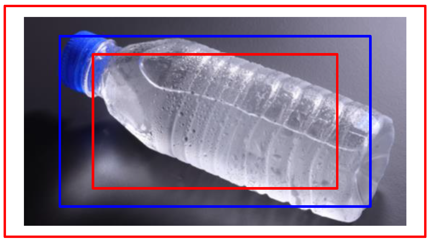
2.3. Intersection over Union (IoU) Loss Functions

The Intersection over Union (IoU) loss [34] first obtains the ratio of intersection and union between the predicted box A and ground truth box B, as follows:

$$IoU=\frac{\left|A\cap B\right|}{\left|A\cup B\right|}.$$

(1)

The IoU loss is defined as:

$$L_{IoU}=1-IoU.$$

(2)

If the predicted box and ground truth box fully overlap, IoU is equal to 1, meaning that a loss value of 0 indicates the highest possible degree of overlapping between these two boxes. Figure 2 shows three common ways of overlapping between the predicted box and ground truth box.

In order to solve problems arising when the distance between these two boxes cannot be reflected because the predicted box and ground truth box do not intersect, and to reflect the coincidence degree between them, Stanford scholars introduced a minimum circumscribed rectangle C of the predicted box A and ground truth box B, and propose the GIoU loss [35], on the basis of the IoU loss, as follows:

$$L_{GIoU}=1-IoU+\frac{C-A \cup B}{C}.$$

(3)

Three different relationships between A, B, and C are shown in Figure 3.

However, the GIoU loss degenerates to the IoU lost when the predicted box A and ground truth box B are of the same width or same height (c.f. Figure 3b,c). Thus, some scholars have modified the penalty term of introducing the minimum circumscribed box in GIoU so as to maximize the overlap area and minimize the standardized distance between the two bounding boxes’ (BBoxes) centers, thus speeding up the convergence process of the loss. The result of this is the DIoU loss [23], defined as follows:

$$L_{DIoU}=1-IoU+\frac{\left(b,b^{gt}\right){\rho }^2}{D^2},$$

(4)

where $b$ and $b^{gt}$ denote the center points of the predicted box and ground truth box, respectively, $\rho$ denotes the Euclidean distance between them, and $D$ denotes the diagonal distance of the minimum closure area that contains both the predicted box and ground truth box.

Another loss function, CIoU, which is used in YOLOv5 for the calculation of the location score of the compound loss [1], considers the aspect ratio of the DIoU loss on the basis of BBoxes, thus further improving the regression accuracy as follows:

$$L_{CIoU}=1-IoU+\frac{\left(b,b^{gt}\right){\rho }^2}{D^2}+\alpha v,$$

(5)

where α denotes the weighting factor and v is used to measure the consistency of the relative proportions of the ground truth box and prediction box. Although the CIoU loss considers the overlap area along with the center distance and aspect ratio of the BBox regression, the difference of the aspect ratio is reflected in its formula, rather than the real difference between the width and height of the two boxes and its confidence, respectively, thus sometimes hindering the effective optimization similarity of the model. This problem is illustrated in Figure 4, where the blue box refers to the ground truth box, while the two red boxes correspond to two different predicted boxes. All three boxes are of the same proportion and have a common center, so the CIoU loss may be inconsistent with the regression object. To solve this problem, in the EIoU loss [36], two optimizations have been made on the basis of the CIoU loss: (i) disassembling the aspect ratio; and (ii) adding a focal loss to spotlight quality anchor boxes. The penalty term of EIoU is to disassemble the impact factors of the aspect ratio on the basis of the penalty term of CIoU and calculate the length and width of the prediction box and anchor box, respectively (the anchor box is obtained according to the object position in the image and is used for making the predicted box). The loss function includes three parts: overlap loss, center distance loss, and width–height loss, as follows:

$$L_{EIoU}=1-IoU+\frac{\left(b,b^{gt}\right){\rho }^2}{C^2}+\frac{\left(w,w^{gt}\right){\rho }^2}{C_w^2}+\frac{\left(h,h^{gt}\right){\rho }^2}{C_h^2} ,$$

(6)

where $w$ and $h$ denote the width and height of the predicted box, $w^{gt}$ and $h^{gt}$ denote the width and height of the ground truth box, and $C_w$ and $C_h$ denote the width and height of the minimum BBox covering the true part of the predicted box. In (6), the first two parts still follow the CIoU logic, but the width–height loss directly minimizes the difference between the width and height of the object box and anchor box, making the convergence faster.

3. Related Work

The object detection models can be generally divided into two main categories depending on the presence or absence of region proposals. The first category includes the two-stage models for object detection, mainly carried out by means of a convolutional neural network (CNN), using region recommendation to identify possible positions of objects in advance by using color edges of the images and other information, and then reducing the complexity of computing through some candidate positions. The two-stage object detection models exhibit high accuracy but lower speed than the single-stage models, appearing later, which calculate the probability of an object being a certain type by direct regression along with obtaining the coordinate value of the object’s position in the image. The models in this second category are generally less accurate, but faster than the two-stage object detection models.

3.1. Two-Stage Object Detection Models

3.1.1. R-CNN

R-CNN [7] is a milestone in the application of CNNs for object detection, realized by region proposals. R-CNN is the first work of the two-stage models, laying a foundation for the development of future models of this type. Before R-CNN, many effective models mainly used complex ensemble systems that fused multiple low-level image features and high-level context information. R-CNN is a simple and scalable object detection model, which obtained the best MAP of 53.3% on VOC2012 due to two main reasons: (i) extracting features from top-down candidate regions using a CNN for object detection and object segmentation; and (ii) using pre-training transfer learning of other auxiliary tasks, which can greatly improve the performance when the size of the dataset is small.

The operation of R-CNN is depicted in Figure 5. First, the image is divided into candidate regions. Then, a CNN is used to extract features from each candidate region. The extracted features are sent to a support vector machine (SVM) classifier [37] to determine the class they belong to. Finally, the position of the candidate box is refined by a BBox regression.

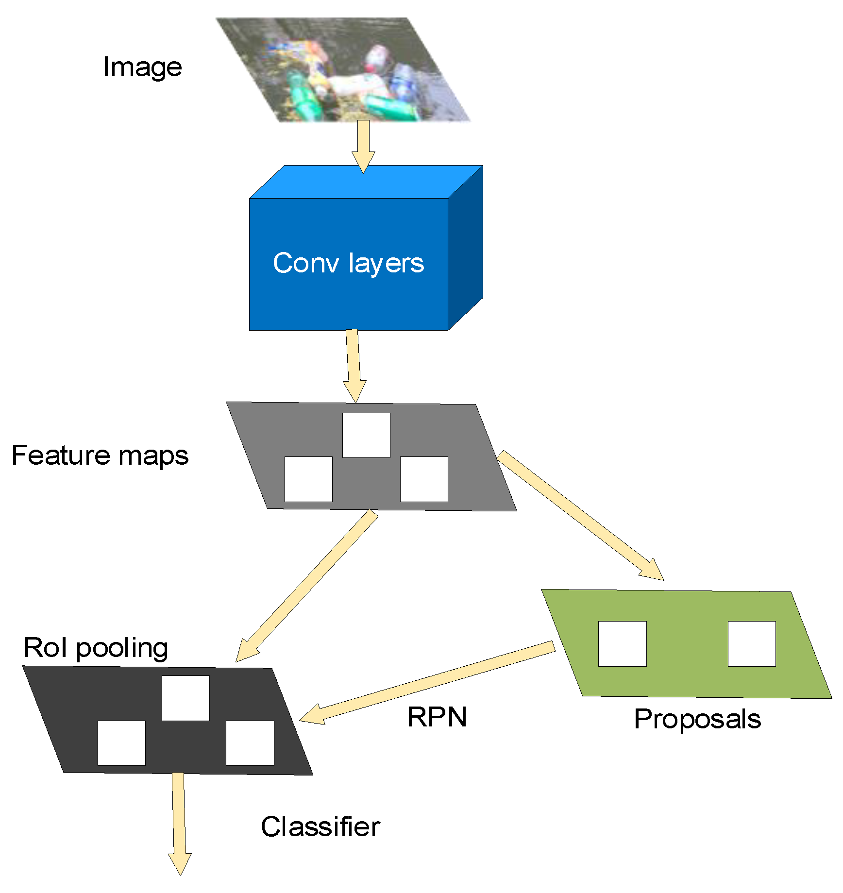
3.1.2. Faster R-CNN

Faster R-CNN [10] consists of two main modules, as shown in Figure 6. The first module is a Region Proposal Network (RPN) used for extracting the BBoxes, and the second one is a Fast R-CNN object detector operating on the candidate boxes. An attention mechanism is used to pay more attention to particular parts of the images processed. First, the features of the input data are extracted by means of a CNN. Then, the RPN module is used to generate a large number of anchor boxes, cut and filter them, and then judge whether an anchor is a foreground or background. This is followed by mapping of the serial interface, suggested to the last convolution, generating a feature map of fixed size, and performing further training.

3.2. Single-Stage Object Detection Models

3.2.1. Single Shot MultiBox Detector (SSD)

The feature extraction network of SSD is derived from the improvement of the VGG16 network [38]. The feature map of small features is increased by adding several groups of convolutional layers behind the VGG16 network. The multi-scale detection method adopted by SSD is to gradually use the convolution operation with a step size of 2 on the large feature map output by the VGG16 network, so as to generate feature maps of two scales. The larger of the two scales is used to identify small objects, while the smaller one is used to identify large objects. This approach leads to improving the detection accuracy of small objects.

Ideologically, SSD draws on the Faster R-CNN’s anchor idea, but also refers to the YOLO’s regression idea. SSD performs regression calculations through the multi-scale regional features of all convolutional layers, which allows it to achieve a good balance between detection accuracy and speed.

3.2.2. YOLO

YOLOv1 [15], YOLOv2 [16], YOLOv3 [17] are general object detection models proposed by Redmon et al. YOLOv4 [18] is an improvement of YOLOv3, proposed by Bochkovskiy et al. It summarizes almost all the object detection techniques, which are then screened, arranged, and combined to verify which one is the more effective for use. Based on YOLOv4, YOLOv5 [20] undergoes scaling, adjustment of color space, and enhancement of Mosaic data. At the same time, the anchor box of YOLOv5 is automatically learned based on the training set, whereas YOLOv4 does not have an adaptive anchor box. The activation functions adopted by YOLOv5 include Leaky ReLU [39] (used at the middle layer) and Sigmoid (used at the final detection layer), whereas YOLOv4 uses Leaky ReLU and Mish activation functions. YOLOv5 uses two optimization functions—the adaptive moment estimation (Adam) and stochastic gradient descent (SGD) (used by default)–with presetting of the matching training super-parameters for both. YOLOv4 only uses the SGD optimization function. The compound loss function of YOLOv5 contains classes loss, objectness loss, and location loss, whereby the latter is calculated using the CIoU loss and the other two losses are calculated using the Binary Cross-Entropy with Logits Loss (BCEWithLogitsLoss) (https://pytorch.org/docs/master/generated/torch.nn.BCEWithLogitsLoss.html) (accessed on 3 November 2022) [1]. Differently, YOLOv4 uses only the CIoU loss.

So far, based on YOLOv5, Ultralytics has produced a total of five models—YOLOv5n, YOLOv5s, YOLOv5m, YOLOv5l, and YOLOv5x. YOLOv5m, YOLOv5l, and YOLOv5x use neural networks with the smallest depth and widest feature map width, on the basis of YOLOv5s. The YOLOv5_CBS model, proposed in this paper, mainly improves the YOLOv5s model.

Figure 7 presents the YOLOv5 structure consisting of four parts—input, backbone, neck, and prediction. The YOLOv5 input uses the Mosaic data enhancement method, which is a reference to the CutMix [40] data enhancement method proposed at the end of 2019. On its basis, four images are stitched using random scaling, random cropping, and random arrangement, which improves the detection of small objects (a small object is defined as a detected object with size between 0*0 and 32*32). At the same time, YOLOv5 also adopts adaptive anchor box computing; in different datasets, anchor boxes are initially set with different sizes. In the process of network training, the network outputs the predicted box based on the initial anchor box, compares it with the ground truth box, continuously calculates the gap between them, and then reversely updates and iterates the network parameters. YOLOv5 also adopts adaptive image scaling, so that its reasoning is faster and its object detection speed is also improved. YOLOv5’s backbone section combines various new approaches including: CSPDarknet53 [41], Mish activation function [42], Dropblock [43], and others. YOLOv5’s neck uses PAN and FPN network structures. FPN is a top-down model, which transfers and fuses the high-level feature information from top sampling to obtain a feature map for prediction, while PAN adds bottom-up route enhancement and adaptive feature pooling. Moreover, YOLOv5 uses a non-maximum suppression (NMS) to complete the screening of many object boxes during the post-processing of object detection.

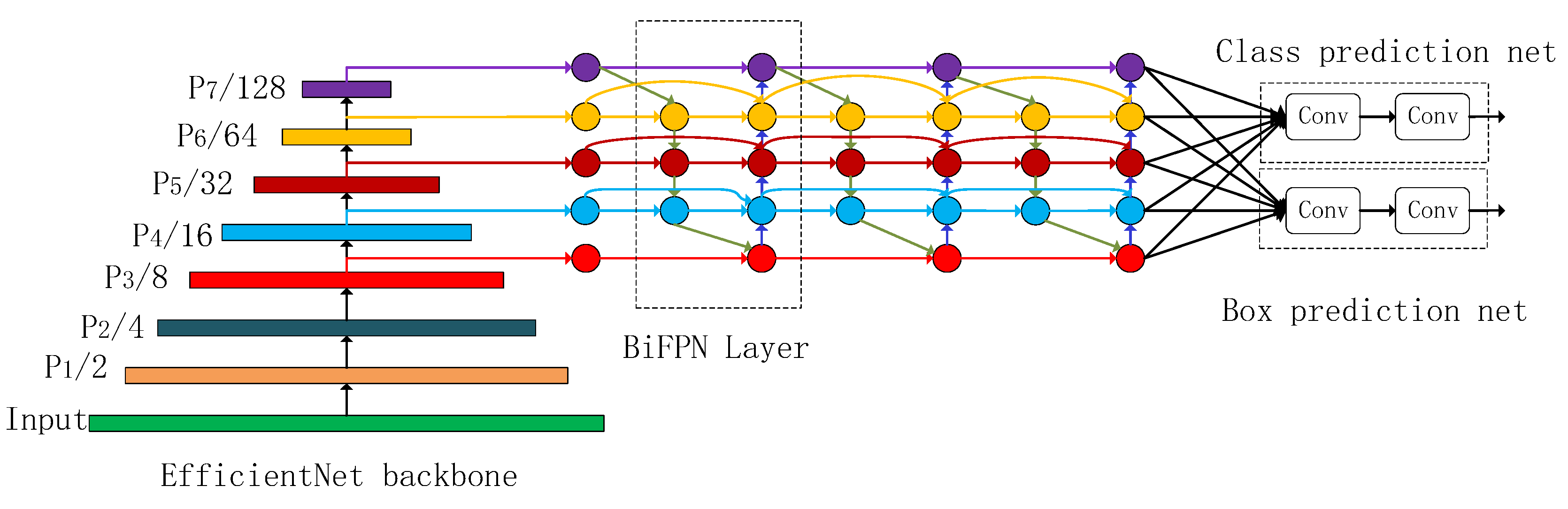
3.2.3. EfficientDet

EfficientDet [44] is a series of eight object detection algorithms (D0 to D7) published in November 2019. With different equipment constraints, it can achieve state-of-the-art results with always better efficiency than the prior models used under extensive resource constraints. Especially in the case of a single model and a single scale, EfficientDet-D7 achieves average precision of 52.2% on the Microsoft Common Objects in Context (COCO) test equipment with 52M parameters and 325B floating point of operations (FLOPs), which represents a significant improvement over the previously used models (i.e., FLOPs are reduced by a factor of 13 to 42).

Firstly, EfficientDet proposes a weighted bidirectional feature pyramid network (BiFPN), which allows simple and fast multi-scale feature integration. Secondly, EfficientDet proposes a compound feature pyramid network scaling method, which uniformly scales the resolution, depth and width, feature network, and box/class prediction network of the backbone. Figure 8 depicts the EfficientDet-D0 structure.

4. Proposed YOLOv5_CBS Model

Based on YOLOv5, this paper proposes a novel YOLOv5_CBS model, shown in Figure 9, with the following improvements described in detail in the subsections below: (i) adding a coordinate attention (CA) mechanism after the original C3 module (similarly to [22], but without compressing the number of channels in the bottleneck, thus forming a new C3-CA-Uncompress Bottleneck (CCUB) module, which is used instead of the original C3 module); (ii) replacing the original PAN network structure with a BiFPN structure; and (iii) replacing the CIoU loss function, which is originally used in YOLOv5 for the calculation of location score of the compound loss, with the SIoU loss function.

4.1. Using a SIoU Loss Function

The traditional object detection loss function depends on the aggregation of regression indexes of the BBox, such as the distance, overlap area, and aspect ratio between the predicted box and ground truth box. However, the methods proposed and used so far have not considered the direction of the mismatch between the ground truth box and the predicted box [24]. This deficiency causes slow convergence and low efficiency because the predicted box may wander around in the training process, eventually producing a worse model. To solve this problem, in May 2022, Gevorgyan proposed the SIoU loss [24], consisting of four basic functions, namely the angle cost, distance cost, shape cost, and IoU cost.

The angle cost is calculated as follows:

$$\Lambda =1-2\times si{n}^2\left(arcsin\left(\frac{c_h}{\sigma }\right)-\frac{\pi }{4}\right),$$

(7)

where $c_h$ denotes the height difference between the center points of the ground truth box and predicted box, and $\sigma$ denotes the distance between the center points of the ground truth and predicted box.

The distance cost is calculated as follows:

$$\Delta ={{\displaystyle \sum }}_{t=x,y}\left(1-e^{-\gamma {\rho }_t}\right) ,$$

(8)

where

$${\rho }_x={\left(\frac{b_{c_x}^{gt}-b_{c_x}}{c_w}\right)}^2;{\rho }_y={\left(\frac{b_{c_y}^{gt}-b_{c_y}}{c_h}\right)}^2;\gamma =2-\Lambda ,$$

(9)

$b_{c_x}^{gt}$ and $b_{c_y}^{gt}$ are the coordinates of the center point of the ground truth box, $b_{c_x}$ and $b_{c_y}$ are the coordinates of the center point of the predicted box, and

$$c_w=\mathit{max} \left(b_{c_x}^{gt},b_{c_x}\right)-\mathit{min} \left(b_{c_x}^{gt},b_{c_x}\right) ;$$

(10)

$$c_h=\mathit{max} \left(b_{c_y}^{gt},b_{c_y}\right)-\mathit{min} \left(b_{c_y}^{gt},b_{c_y}\right).$$

(11)

The shape cost is calculated as follows:

$$\Omega ={\displaystyle \sum }_{t=w,h}{\left(1-e^{-{\omega }_t}\right)}^{\theta },$$

(12)

where $\theta$ represents the degree of attention that should be paid to the shape cost and

$${\omega }_w=\frac{\left|w-w^{gt}\right|}{\mathit{max}\left(w, w^{gt}\right)} ; {\omega }_h=\frac{\left|h-h^{gt}\right|}{\mathit{max}\left(h, h^{gt}\right)},$$

(13)

where $w$ and $h$, and $w^{gt}$ and $h^{gt}$, denote the width and height of the predicted box and ground truth box, respectively.

The SIoU loss function is defined as

$$Los{s}_{SIou}=1-IoU+\frac{\Delta +\Omega }{2}.$$

(14)

Since the SIoU loss introduces the vector angle between the required regressions, it can accelerate the convergence speed and improve the regression accuracy. These are the main reasons why the proposed YOLOv5_CBS model adopts the SIoU loss as its loss function.

4.2. Using a Coordinate Attention

Coordinate attention (CA) [21] encodes the relationship between channels and long-term dependency through accurate location information. The specific operations used are the coordinate information embedding and the CA generation.

The global pooling method is usually used for the global coding of channel attention code space information, however, with it, it is difficult to save the position information because it compresses the global space information into the channel descriptor. To enable the attention module to capture the remote spatial interaction with accurate position information, the global pooling is decomposed by the following formula and transformed into a one-to-one dimensional feature code operation:

$$z_c=\frac{1}{H\times W}{\displaystyle \sum }_{i=1}^H{\displaystyle \sum }_{j=1}^W{x}_c\left(i,j\right),$$

(15)

where $H$ and $W$ denote the height and width of the polling kernel, $x_c$ denotes the input of channel $C$, and $z_c$ denotes the output of channel $C$. Firstly, each channel is coded along horizontal and vertical coordinates by a pooling kernel with the size of $\left(H,1\right)$ or $\left(1,W\right)$. Then, the input feature map is divided into width and height directions for global average pooling. In each direction, the feature map is, respectively, obtained as follows:

$$z_c^h\left(h\right)=\frac{1}{W}{\displaystyle \sum }_{0\le i<W}{x}_c\left(h,i\right); z_c^w\left(w\right)=\frac{1}{H}{\displaystyle \sum }_{0\le j<H}{x}_c\left(j,w\right).$$

(16)

By means of (16), features along two spatial directions are aggregated to obtain a pair of directional sensing feature maps. The two transformations in (16) also allow CA to capture the long-term dependence along one spatial direction and save the accurate position information along another spatial direction, which helps the network to position the objects of interest more accurately.

Through the transformations performed by the first operation (i.e., the coordinate information embedding), CA can better obtain the global receptive field and encode the accurate position information. To make use of the resulting representation, a second operation, called CA generation, performs concatenation on the above transformations, and then performs transformation by using the following convolution function:

$$f=\delta \left(F_1\left(\left[z^h,z^w\right]\right)\right),$$

(17)

where $F_1$ denotes the characteristic diagram after batch normalization, $z^h$ denotes the output of the channel at height $h$, and $z^w$ denotes the output of the channel at width $w$. The concatenation performed along the spatial dimension is a nonlinear activation function and an intermediate feature mapping for encoding spatial information in the horizontal and vertical directions. Then, it is decomposed into two separate tensor sums along the spatial dimension, whereby the sums are transformed into tensors with the same number of channels as the input by using the sums of other two convolution transformations. The two convolutions and Sigmoid activation function for $f^h$ and $f^w$ are used to obtain the attention weights $g^h$ and $g^w$ in height and width, respectively, as follows:

$$g^h=\sigma \left(F_h\left(f^h\right)\right) ; g^w=\sigma \left(F_w\left(f^w\right)\right),$$

(18)

where $f^h$ denotes the intermediate feature map that encodes spatial information in the vertical direction, $f^w$ denotes the intermediate feature map that encodes spatial information in the horizontal direction, $\sigma$ denotes the Sigmoid function, and $F_h$ and $F_w$ denote a 1 × 1 convolutional transformation in the horizontal and vertical direction, respectively.

In order to reduce the complexity and computational cost, an appropriate reduction ratio is usually applied to reduce the number of channels. Then, the output sums are expanded, and attention weights are applied, respectively. Finally, the CA output can be written as follows:

$$y_c\left(i,j\right)=x_c\left(i,j\right)\times g_c^h\left(i\right)\times g_c^w\left(j\right).$$

(19)

In the proposed YOLOv5_CBS model, the CA attention mechanism is added after the original C3 module of YOLOv5, as suggested in [22]. However, the difference between the C3-CA-Uncompress Bottleneck (CCUB) module (Figure 10), used in the proposed YOLOv5_CBS model, and the C3CA module proposed in [22], is that the CCUB module does not compress the number of channels in the bottleneck.

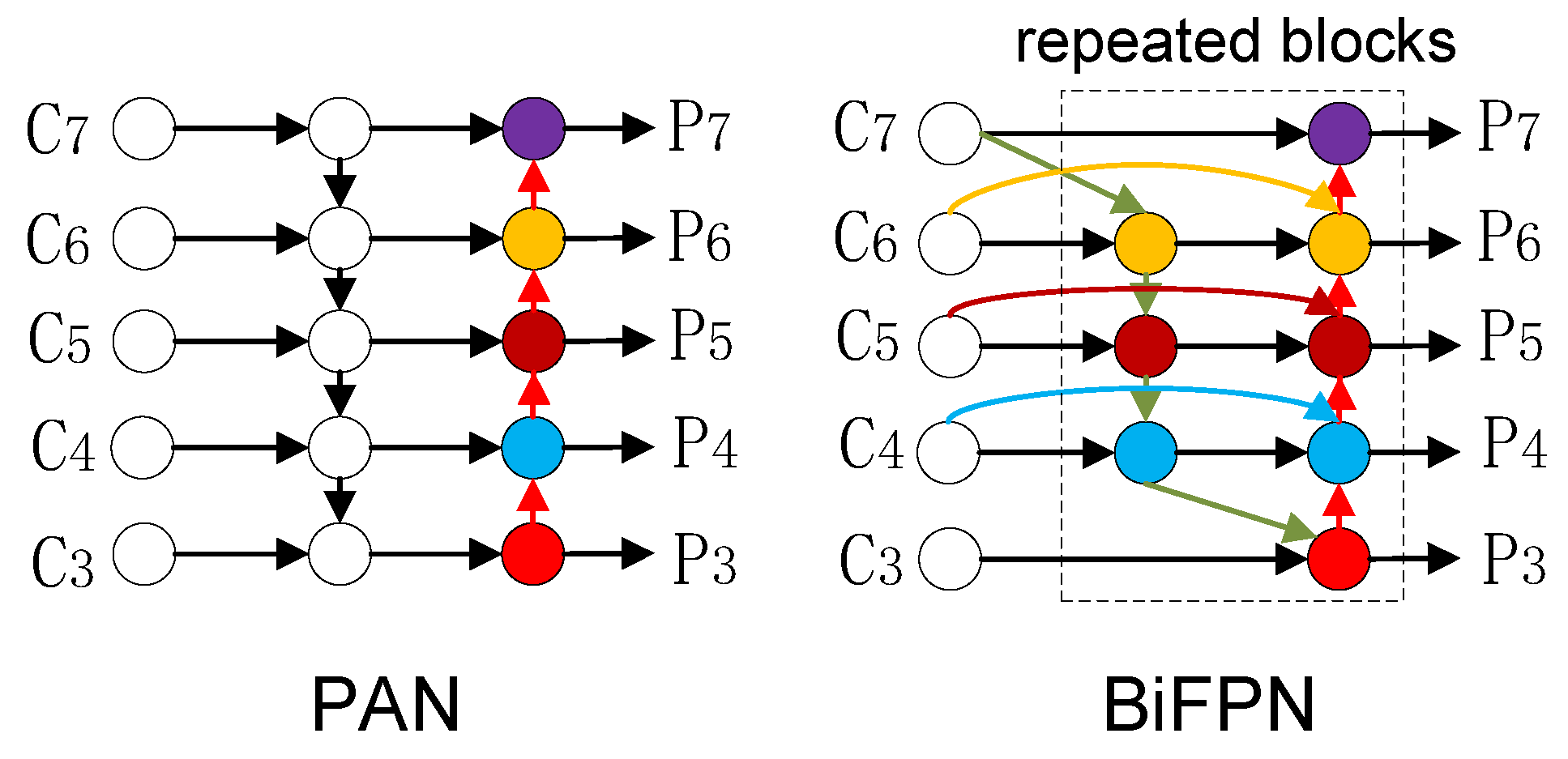
4.3. Using a BiFPN

In the proposed YOLOv5_CBS model, the original PAN network structure [45] of YOLOv5s is replaced with a BiFPN structure [46], as proposed by Du and Jiao in [47] for enhancing the depth of information mining and improving the feature extraction capability of the model. In addition, this replacement allows realization of two-way fusion of top-down and bottom-up deep and shallow features, thus enhancing the transfer of feature information between different network layers and improving the detection performance of the model. Compared to PAN, improvements of BiFPN, shown in Figure 11, include: (i) deletion of all network nodes with only one input edge (as these have less contribution with respect to fusing different features, which leads to a simplified two-way network); (ii) adding an extra edge between an input and output node positioned at the same level (so as to integrate more functions without increasing the cost); (iii) using different top-down and bottom-up paths (each two-way path, i.e., top-down and bottom-up, is regarded as an elementary network layer, which is repeated many times to enable more advanced functional convergence).

The use of BiFPN strengthens the effect of feature fusion between different scales by downSample, upSample, and spanning links. In the proposed YOLOv5_CBS model, the Concat method is used for feature fusion, which avoids possible information loss and is not limited by the number of channels in the feature map. In addition, BiFPN can make better use of the correlation between depth maps of different scales.

5. Experiments and Results

5.1. Datasets

The experiments were carried out on two datasets used for river garbage object detection. The first one is a private dataset provided by respective units in Tangshan City, Hebei Province, China. The other one is the FloW-Img public dataset [48] provided by researchers from Mila Laboratory, Tsinghua University, China, and Northwestern Polytechnical University, China.

The private dataset contains 2400 images with a resolution of 416×416, including 3510 floating garbage objects. In order to meet the requirements of the experiments, the dataset was first converted into the VOC2007 format and then annotated by means of the LabelImg software (https://github.com/tzutalin/labelImg) (accessed on 15 August 2022). In the conducted experiments, the original images of the dataset were used without any preprocessing, such as sharpening. Sample images of this dataset are shown in Figure 12.

The FloW-Img public dataset contains 2000 images with a resolution of 1280 × 720, including 5271 floating garbage objects, all labeled [48]. In the experiments, the original images of the dataset were used without any preprocessing. Sample images of this dataset are shown in Figure 13.

In the conducted experiments, in each dataset, the images were divided into three separate subsets, based on the number of object labels, whereby the training subset accounted for 60%, the validation subset for 20%, and the test subset for 20% of the total number of labels. The specific number of labels in each subset is shown in

Table 1. Splitting of datasets into training, validation, and test subsets.

	Private Dataset	Flow-Img Dataset
Training subset	2106 labels	3163 labels
Validation subset	702 labels	1054 labels
Test subset	702 labels	1054 labels

for each dataset used. Using these percentages, the images in each dataset were split randomly five times in different subset conglomerations so as to eliminate the test contingency. The obtained results are shown under the corresponding experiment number in Section 5.4.

5.2. Experiments Setup

Experiments were conducted on a PC with the Windows 11 operating system, Intel TM i5-11400F CPU, GeForce RTX3060 GPU, and 12 GB video memory, by using CUDA11.3 for training acceleration, PyTorch 1.11 deep learning framework for training, input image size of 640 × 640, initial learning rate of 0.01, final learning rate of 0.1, SGD optimizer with 0.937 momentum, and training batch size of 8, as shown in

Table 2. Experiments setup components.

Component	Name/Value
Operating system	Windows 11
CPU	Intel TM i5-11400F
GPU	GeForce RTX3060
Video memory	12 GB
Training acceleration	CUDA 11.3
Deep learning framework for training	PyTorch 1.11
Input image size	640 × 640
Initial learning rate	0.01
Final learning rate	0.1
Optimizer	SGD
Optimizer momentum	0.937
Training batch size	8

.

5.3. Evaluation Metrics

In the conducted experiments, the object detection performance of the proposed YOLOv5_CBS model was compared to that of four state-of-the-art models, namely Faster R-CNN, YOLOv3, YOLOv4, and YOLOv5, based on precision and recall, which are commonly used evaluation metrics for detection problems.

Precision refers to the proportion of correct object detections to all (true and false) positive detections, as follows:

$$precision=\frac{TP}{TP+FP},$$

(20)

where TP (true positive) refers to the number of correct positive outcomes (object detections) and FP (false positive) refers to the number of incorrect positive outcomes.

Recall refers to the proportion of correct object detections to the actual number of all objects, as follows:

$$recall=\frac{TP}{TP+FN},$$

(21)

where FN refers to the number of incorrect negative outcomes.

For the performance evaluation of the compared models, the F1 score and average precision were used as the main metrics because they take into account both precision and recall. F1 score is the harmonic mean of precision and recall, defined as follows:

$$F1=\frac{2\ast precision\ast recall}{precision+recall}.$$

(22)

The higher the F1 score, the more robust the model.

Average precision (AP) represents the mean of the detector in all recalls, corresponding to the area under the precision–recall curve, which can be expressed as:

$$AP={{\displaystyle \int }}_0^{1}p\left(r\right)\mathrm{d}r,$$

(23)

where $p\left(r\right)$ denotes the precision function of recall ($r$).

5.4. Results

In the conducted experiments, the precision–recall curves were first created for each of the compared models, using each dataset, based on the obtained values of recall and precision. Then, these curves were used to calculate the AP of each model, separately for each of the five conducted experiments, based on (23). The calculated AP values of each model in each of the five experiments, conducted on each dataset, are presented in

Table 3. Average precision (%) of compared models on private dataset.

Model	Experiment 1	Experiment 2	Experiment 3	Experiment 4	Experiment 5
Faster R-CNN	76.16	78.63	75.76	78.11	75.47
YOLOv3	80.09	81.34	79.28	81.46	82.43
YOLOv4	80.90	82.73	80.44	81.83	82.97
YOLOv5	85.96	88.37	87.73	86.44	88.28
YOLOv5_CBS	89.82	91.92	90.38	90.96	91.16

and

Table 4. Average precision (%) of compared models on FLOW-Img public dataset.

Model	Experiment 1	Experiment 2	Experiment 3	Experiment 4	Experiment 5
Faster R-CNN	78.34	77.83	79.16	80.12	78.96
YOLOv3	82.27	83.65	83.01	84.83	83.93
YOLOv4	87.65	87.90	86.22	88.52	85.81
YOLOv5	90.51	90.93	89.56	92.15	89.76
YOLOv5_CBS	91.68	92.65	91.46	93.77	91.34

. Then, F1 score, was used, separately for each model in each of the five experiments, conducted on each dataset. The calculated F1 score values of each model in each of the five experiments, conducted on each dataset, are presented in

Table 5. F1 score of compared models on private dataset.

Model	Experiment 1	Experiment 2	Experiment 3	Experiment 4	Experiment 5
Faster R-CNN	0.7003	0.7198	0.6954	0.7146	0.6919
YOLOv3	0.7534	0.7642	0.7379	0.7613	0.7704
YOLOv4	0.7694	0.7859	0.7678	0.7805	0.7839
YOLOv5	0.8049	0.8361	0.8277	0.8204	0.8314
YOLOv5_CBS	0.8564	0.8759	0.8636	0.8675	0.8712

and

Table 6. F1 score of compared models on FLOW-Img public dataset.

Model	Experiment 1	Experiment 2	Experiment 3	Experiment 4	Experiment 5
Faster R-CNN	0.7102	0.7118	0.7249	0.7367	0.7179
YOLOv3	0.7768	0.7913	0.7880	0.7994	0.7902
YOLOv4	0.8490	0.8504	0.8413	0.8572	0.8392
YOLOv5	0.8763	0.8796	0.8992	0.8974	0.8637
YOLOv5_CBS	0.8935	0.9048	0.8957	0.9186	0.8904

. The corresponding values of AP, and separately of F1 score, were then averaged across all five experiments to obtain the final AP and F1 score result for each model on each dataset, as summarized in

Table 7. Performance comparison of models on private dataset.

Model	Recall	F1 Score	AP (%)	Training Time (h)	FPS
Faster R-CNN	0.604	0.7044	76.83	18.4	11.6
YOLOv3	0.667	0.7574	80.92	8.6	30.9
YOLOv4	0.693	0.7775	81.77	7.5	40.1
YOLOv5	0.837	0.8241	87.36	2.2	95.2
YOLOv5_CBS	0.885	0.8669	90.85	2.9	75.2

and

Table 8. Performance comparison of models on FLOW-Img public dataset.

Model	Recall	F1 Score	AP (%)	Training Time (h)	FPS
Faster R-CNN	0.621	0.7203	78.88	16.1	10.5
YOLOv3	0.685	0.7891	83.54	7.5	31.7
YOLOv4	0.828	0.8474	87.22	6.5	39.8
YOLOv5	0.861	0.8832	90.58	1.6	96.2
YOLOv5_CBS	0.865	0.9006	92.18	2.1	76.9

.

According to the results obtained on the private dataset shown in Table 7, the proposed YOLOv5_CBS model outperforms all four state-of-the-art models with respect to recall, average precision (AP), and F1 score achieved. More specifically, Faster R-CNN, YOLOv3, YOLOv4, and YOLOv5 are outperformed, respectively, by 0.281, 0.218, 0.192, and 0.048 points in terms of recall, by 14.02, 9.93, 9.08, and 3.49 points in terms of AP, and by 0.1625, 0.1095, 0.0894, and 0.0428 points in terms of F1 score. With respect to the training time and frame rate (measured in frames per second, FPS), the proposed YOLOv5_CBS model closely follows the winner, i.e., the original YOLOv5 model, by significantly outperforming the other three models, i.e., Faster R-CNN, YOLOv3, and YOLOv4.

According to the results obtained on the FloW-Img public dataset shown in Table 8, the proposed YOLOv5_CBS model outperforms all four state-of-the-art models with respect to recall, average precision (AP), and F1 score achieved on this dataset too. More specifically, Faster R-CNN, YOLOv3, YOLOv4, and YOLOv5 are outperformed, respectively, by 0.244, 0.180, 0.037, and 0.004 points in terms of recall, by 13.30, 8.64, 4.96, and 1.60 points in terms of AP, and by 0.1803, 0.1115, 0.0532, and 0.0174 points in terms of F1 score. With respect to the training time and frame rate, the proposed YOLOv5_CBS model again closely follows the winner, i.e., the original YOLOv5 model, by significantly outperforming the other three models, i.e., Faster R-CNN, YOLOv3, and YOLOv4.

Although the proposed YOLOv5_CBS model outperforms all considered state-of-the-art models based on all evaluation metrics used and on both datasets, the initial observations reveal some shortcomings. For instance, it seems that YOLOv5_CBS is not so effective for the detection of floating objects when reflections on the water surface exist (in which case part of the prediction box may treat the reflection as an object too, or results in a bigger prediction box which should not actually include the reflection, c.f., B instances in Figure 14), or if multiple small objects are present in the images, or when the density of the target objects is high (resulting in low detection rates and low confidence levels, c.f., A instances in Figure 14).

6. Conclusions

In order to better detect floating garbage in rivers, this paper has proposed a novel model, called YOLOv5_CBS, based on the YOLOv5 model. Firstly, a coordinate attention (CA) mechanism has been added to the original C3 module of YOLOv5 (similarly to [22], but without compressing the number of channels in the bottleneck), forming a new C3-CA-Uncompress Bottleneck (CCUB) module so as to increase the receptive domain and make the model pay more attention to important parts of the images. Secondly, in order to enable the model to extract features more quickly and effectively and reduce the computation of redundant information of features, the original feature fusion network, PAN, of YOLOv5 has been replaced by BiFPN, as proposed in [47]. Thirdly, on the premise of keeping the fast prediction ability of YOLOv5, for the calculation of location score of the compound loss, the CIoU loss function has been replaced with the SIoU loss function, so as to improve the convergence speed and regression accuracy of the model. A series of experiments, conducted on two datasets, confirmed that these improvements integrated into YOLOv5 can indeed help achieve better detection of garbage objects floating in rivers, which has also been demonstrated with respect to three other state-of-the-art models (Faster R-CNN, YOLOv3, and YOLOv4), in terms of recall, average precision, and F1 score.

However, due to the use of the CA mechanism by the proposed YOLOv5_CBS model, it has higher computational complexity and requires more time for training than the original YOLOv5 model (c.f. Table 7 and Table 8). In the view of this, in the future, we plan to introduce some specially designed lightweight modules into the model to increase its object detection speed. In addition, we also plan to work on improving the small-object detection ability of the model by employing additional techniques and methods, such as the improved feature fusion method (PB-FPN) proposed in [49] for small object detection based on PAN and BiFPN.

References

- Huang, J.; Jiang, X.; Jin, G. Detection of River Floating Debris in UAV Images Based on Improved YOLOv5. In Proceedings of the 2022 International Joint Conference on Neural Networks (IJCNN), Padua, Italy, 18–23 July 2022; pp. 1–8. [Google Scholar]
- Viola, P.A.; Jones, M.J. Rapid Object Detection using a Boosted Cascade of Simple Features. In Proceedings of the Computer Vision and Pattern Recognition, 2001, CVPR 2001, Kauai, HI, USA, 8–14 December 2001. [Google Scholar]
- Dalal, N.; Triggs, B. Histograms of oriented gradients for human detection. In Proceedings of the 2005 IEEE computer society conference on computer vision and pattern recognition (CVPR’05), San Diego, CA, USA, 20–25 June 2005; pp. 886–893. [Google Scholar]
- Felzenszwalb, P.F.; Mcallester, D.A.; Ramanan, D. A discriminatively trained, multiscale, deformable part model. In Proceedings of the 2008 IEEE Conference on Computer Vision and Pattern Recognition, Anchorage, AK, USA, 23–28 June 2008. [Google Scholar]
- Felzenszwalb, P.F.; Girshick, R.B.; McAllester, D.; Ramanan, D. Object detection with discriminatively trained part-based models. IEEE Trans. Pattern Anal. Mach. Intell. 2010, 32, 1627–1645. [Google Scholar] [CrossRef] [PubMed]
- Felzenszwalb, P.F.; Girshick, R.B.; McAllester, D. Cascade object detection with deformable part models. In Proceedings of the 2010 IEEE Computer Society Conference on Computer Vision and Pattern Recognition, San Francisco, CA, USA, 13–18 June 2010; pp. 2241–2248. [Google Scholar]
- Girshick, R.; Donahue, J.; Darrell, T.; Malik, J. Rich feature hierarchies for accurate object detection and semantic segmentation. In Proceedings of the IEEE Conference on Computer Vision and Pattern Recognition, Columbus, OH, USA, 23–28 June 2014; pp. 580–587. [Google Scholar]
- He, K.; Zhang, X.; Ren, S.; Sun, J. Spatial pyramid pooling in deep convolutional networks for visual recognition. IEEE Trans. Pattern Anal. Mach. Intell. 2015, 37, 1904–1916. [Google Scholar] [CrossRef] [PubMed]
- Girshick, R. Fast R-CNN. In Proceedings of the 2015 IEEE International Conference on Computer Vision (ICCV), Santiago, Chile, 7–13 December 2015; pp. 1440–1448. [Google Scholar]
- Ren, S.; He, K.; Girshick, R.; Sun, J. Faster R-CNN: Towards Real-Time Object Detection with Region Proposal Networks. IEEE Trans. Pattern Anal. Mach. Intell. 2017, 39, 1137–1149. [Google Scholar] [CrossRef]
- Dai, J.; Li, Y.; He, K.; Sun, J. R-fcn: Object detection via region-based fully convolutional networks. Adv. Neural Inf. Process. Syst. 2016, 29. Available online: https://arxiv.org/abs/1605.06409 (accessed on 26 July 2022).
- Li, Z.; Peng, C.; Yu, G.; Zhang, X.; Deng, Y.; Sun, J. Light-head r-cnn: In defense of two-stage object detector. arXiv 2017, arXiv:1711.07264. [Google Scholar]
- Lin, T.-Y.; Dollár, P.; Girshick, R.; He, K.; Hariharan, B.; Belongie, S. Feature pyramid networks for object detection. In Proceedings of the IEEE Conference on Computer Vision and Pattern Recognition, Honolulu, HI, USA, 21–26 July 2017; pp. 2117–2125. [Google Scholar]
- Liu, W.; Anguelov, D.; Erhan, D.; Szegedy, C.; Reed, S.; Fu, C.-Y.; Berg, A.C. Ssd: Single shot multibox detector. In Proceedings of the European Conference on Computer Vision, Amsterdam, The Netherlands, 8–16 October 2016; pp. 21–37. [Google Scholar]
- Redmon, J.; Divvala, S.; Girshick, R.; Farhadi, A. You Only Look Once: Unified, Real-Time Object Detection. In Proceedings of the 2016 IEEE Conference on Computer Vision and Pattern Recognition (CVPR), Las Vegas, NV, USA, 27–30 June 2016; pp. 779–788. [Google Scholar]
- Redmon, J.; Farhadi, A. YOLO9000: Better, Faster, Stronger. In Proceedings of the 2017 IEEE Conference on Computer Vision and Pattern Recognition (CVPR), Honolulu, HI, USA, 21–26 July 2017; pp. 6517–6525. [Google Scholar]
- Redmon, J.; Farhadi, A. Yolov3: An incremental improvement. arXiv 2018, arXiv:1804.02767. [Google Scholar]
- Bochkovskiy, A.; Wang, C.-Y.; Liao, H.-Y.M. Yolov4: Optimal speed and accuracy of object detection. arXiv 2020, arXiv:2004.10934. [Google Scholar]
- Wang, C.-Y.; Bochkovskiy, A.; Liao, H.-Y.M. Scaled-yolov4: Scaling cross stage partial network. In Proceedings of the IEEE/cvf Conference on Computer Vision and Pattern Recognition, Nashville, TN, USA, 20–25 June 2021; pp. 13029–13038. [Google Scholar]
- Zhu, X.; Lyu, S.; Wang, X.; Zhao, Q. TPH-YOLOv5: Improved YOLOv5 based on transformer prediction head for object detection on drone-captured scenarios. In Proceedings of the IEEE/CVF International Conference on Computer Vision, Montreal, QC, Canada, 10–17 October 2021; pp. 2778–2788. [Google Scholar]
- Hou, Q.B.; Zhou, D.Q.; Feng, J.S.; Ieee Comp, S.O.C. Coordinate Attention for Efficient Mobile Network Design. In Proceedings of the 2021 IEEE/CVF Conference on Computer Vision and Pattern Recognition, CVPR, Nashville, TN, USA, 20–25 June 2021; pp. 13708–13717. [Google Scholar]
- Li, J.; Liu, C.; Lu, X.; Wu, B. CME-YOLOv5: An Efficient Object Detection Network for Densely Spaced Fish and Small Targets. Water 2022, 14, 2412. [Google Scholar] [CrossRef]
- Zheng, Z.; Wang, P.; Liu, W.; Li, J.; Ye, R.; Ren, D. Distance-IoU loss: Faster and better learning for bounding box regression. In Proceedings of the AAAI Conference on Artificial Intelligence, New York, NY, USA, 7–12 February 2020; pp. 12993–13000. [Google Scholar]
- Gevorgyan, Z. SIoU Loss: More Powerful Learning for Bounding Box Regression. arXiv 2022, arXiv:2205.12740. [Google Scholar]
- Bello, I.; Zoph, B.; Vaswani, A.; Shlens, J.; Le, Q.V. Attention augmented convolutional networks. In Proceedings of the IEEE/CVF International Conference on Computer Vision, Seoul, Korea, 27 October–2 November 2019; pp. 3286–3295. [Google Scholar]
- Choromanski, K.; Likhosherstov, V.; Dohan, D.; Song, X.; Gane, A.; Sarlos, T.; Hawkins, P.; Davis, J.; Mohiuddin, A.; Kaiser, L. Rethinking attention with performers. arXiv 2020, arXiv:2009.14794. [Google Scholar]
- Cai, Z.W.; Fan, Q.F.; Feris, R.S.; Vasconcelos, N. A Unified Multi-scale Deep Convolutional Neural Network for Fast Object Detection. In Lecture Notes in Computer Science, Proceedings of the COMPUTER VISION—ECCV 2016, PT IV, Amsterdam, The Netherlands, 11–14 October 2016; Springer Nature: Cham, Switzerland, 2016; pp. 354–370. [Google Scholar]
- Huang, L.; Wang, W.; Chen, J.; Wei, X.-Y. Attention on attention for image captioning. In Proceedings of the IEEE/CVF International Pconference on Computer Vision, Seoul, Korea, 27 October–2 November 2019; pp. 4634–4643. [Google Scholar]
- Jie, H.; Li, S.; Gang, S.; Albanie, S. Squeeze-and-Excitation Networks. IEEE Trans. Pattern Anal. Mach. Intell. 2017, 2011–2023. [Google Scholar] [CrossRef]
- Woo, S.H.; Park, J.; Lee, J.Y.; Kweon, I.S. CBAM: Convolutional Block Attention Module. In Lecture Notes in Computer Science, Proceedings of the COMPUTER VISION—ECCV 2018, PT VII, Munich, Germany, 8–14 September 2018; Springer Nature: Cham, Switzerland, 2018; pp. 3–19. [Google Scholar]
- Wang, Q.; Wu, B.; Zhu, P.; Li, P.; Zuo, W.; Hu, Q. ECA-Net: Efficient Channel Attention for Deep Convolutional Neural Networks. In Proceedings of the 2020 IEEE/CVF Conference on Computer Vision and Pattern Recognition (CVPR), Seattle, WA, USA, 13–19 June 2020; pp. 11531–11539. [Google Scholar]
- Huang, G.; Liu, Z.; Van Der Maaten, L.; Weinberger, K.Q. Densely connected convolutional networks. In Proceedings of the IEEE Conference on Computer Vision and Pattern Recognition, Honolulu, HI, USA, 21–26 July 2017; pp. 4700–4708. [Google Scholar]
- He, K.; Zhang, X.; Ren, S.; Sun, J. Deep residual learning for image recognition. In Proceedings of the IEEE Conference on Computer Vision and Pattern Recognition, Las Vegas, NV, USA, 27–30 June 2016; pp. 770–778. [Google Scholar]
- Zhai, H.; Cheng, J.; Wang, M. Rethink the IoU-based loss functions for bounding box regression. In Proceedings of the 2020 IEEE 9th Joint International Information Technology and Artificial Intelligence Conference (ITAIC), Chongqing, China, 11–13 December 2020; pp. 1522–1528. [Google Scholar]
- Rezatofighi, H.; Tsoi, N.; Gwak, J.; Sadeghian, A.; Reid, I.; Savarese, S. Generalized Intersection Over Union: A Metric and a Loss for Bounding Box Regression. In Proceedings of the 2019 IEEE/CVF Conference on Computer Vision and Pattern Recognition (CVPR), Long Beach, CA, USA, 15–20 June 2019; pp. 658–666. [Google Scholar]
- Zhang, Y.-F.; Ren, W.; Zhang, Z.; Jia, Z.; Wang, L.; Tan, T. Focal and efficient IoU loss for accurate bounding box regression. Neurocomputing 2022, 506, 146–157. [Google Scholar] [CrossRef]
- Niu, X.-X.; Suen, C.Y. A novel hybrid CNN–SVM classifier for recognizing handwritten digits. Pattern Recognit. 2012, 45, 1318–1325. [Google Scholar] [CrossRef]
- Simonyan, K.; Zisserman, A. Very deep convolutional networks for large-scale image recognition. arXiv 2014, arXiv:1409.1556. [Google Scholar]
- Krizhevsky, A.; Sutskever, I.; Hinton, G.E. Imagenet classification with deep convolutional neural networks. Commun. ACM 2017, 60, 84–90. [Google Scholar] [CrossRef]
- Yun, S.; Han, D.; Oh, S.J.; Chun, S.; Choe, J.; Yoo, Y. Cutmix: Regularization strategy to train strong classifiers with localizable features. In Proceedings of the IEEE/CVF International Conference on Computer Vision, Seoul, Korea, 27 October–2 November 2019; pp. 6023–6032. [Google Scholar]
- Wang, C.-Y.; Liao, H.-Y.M.; Wu, Y.-H.; Chen, P.-Y.; Hsieh, J.-W.; Yeh, I.-H. CSPNet: A new backbone that can enhance learning capability of CNN. In Proceedings of the IEEE/CVF Conference on Computer Vision and Pattern Recognition Workshops, Seattle, WA, USA, 13–19 June 2020; pp. 390–391. [Google Scholar]
- Misra, D. Mish: A self regularized non-monotonic neural activation function. arXiv 2019, arXiv:1908.08681. [Google Scholar]
- Ghiasi, G.; Lin, T.-Y.; Le, Q.V. Dropblock: A regularization method for convolutional networks. Adv. Neural Inf. Process. Syst. 2018, 31. Available online: https://proceedings.neurips.cc/paper/2018/file/7edcfb2d8f6a659ef4cd1e6c9b6d7079-Paper.pdf (accessed on 25 July 2022).
- Tan, M.; Pang, R.; Le, Q.V. EfficientDet: Scalable and Efficient Object Detection. In Proceedings of the 2020 IEEE/CVF Conference on Computer Vision and Pattern Recognition (CVPR), Seattle, WA, USA, 13–19 June 2020; pp. 10778–10787. [Google Scholar]
- Liu, S.; Qi, L.; Qin, H.; Shi, J.; Jia, J. Path aggregation network for instance segmentation. In Proceedings of the IEEE Conference on Computer Vision and Pattern Recognition, Salt Lake City, UT, USA, 18–23 June 2018; pp. 8759–8768. [Google Scholar]
- Zhu, L.; Deng, Z.; Hu, X.; Fu, C.-W.; Xu, X.; Qin, J.; Heng, P.-A. Bidirectional feature pyramid network with recurrent attention residual modules for shadow detection. In Proceedings of the European Conference on Computer Vision (ECCV), Munich, Germany, 8–14 September 2018; pp. 121–136. [Google Scholar]
- Du, F.-J.; Jiao, S.-J. Improvement of Lightweight Convolutional Neural Network Model Based on YOLO Algorithm and Its Research in Pavement Defect Detection. Sensors 2022, 22, 3537. [Google Scholar] [CrossRef] [PubMed]
- Cheng, Y.; Zhu, J.; Jiang, M.; Fu, J.; Pang, C.; Wang, P.; Sankaran, K.; Onabola, O.; Liu, Y.; Liu, D. FloW: A Dataset and Benchmark for Floating Waste Detection in Inland Waters. In Proceedings of the IEEE/CVF International Conference on Computer Vision, Montreal, QC, Canada, 10–17 October 2021; pp. 10953–10962. [Google Scholar]
- Liu, H.; Sun, F.; Gu, J.; Deng, L. SF-YOLOv5: A Lightweight Small Object Detection Algorithm Based on Improved Feature Fusion Mode. Sensors 2022, 22, 5817. [Google Scholar] [CrossRef] [PubMed]