Optimal Route Design for Construction Waste Transportation Systems: Mathematical Models and Solution Algorithms

Abstract

A huge amount of construction waste is generated in construction sites every day that needs to be transported by vehicle to disposal facilities for processing. Unlike in most typical transportation problems, once these vehicles are loaded with construction waste, they must travel directly to the disposal facility. Moreover, there are different types of construction waste that may require handling by different disposal facilities. In this paper, we develop a model and algorithm for identifying the optimal transportation routes specific to construction waste transportation. Our results can not only minimize the overall costs for both the logistics company and the contractor but also minimize the distance traveled, thus reducing urban traffic emissions.

1. Introduction

Over 10 billion tons of construction and demolition waste is generated annually worldwide [1]. This vast amount of waste needs to be transported for disposal and recycling, burdening the urban traffic system and incurring high costs. In Hong Kong, for example, an average of 400 trips per day are generated to transport construction waste to the outlying island transfer facilities. According to Lu et al. [2], construction waste transport trucks make 3000 deliveries per day in Hong Kong. As noted by Das and Bhattacharyya [3], waste transportation is not only important but costly; the waste collection process in low- and middle-income countries may account for 80–90% and 50–80%, respectively, of their municipal solid waste management budgets. Considering the ever-increasing labor costs and the high fuel consumption, which also affects the environment, optimizing the design of travel routes to transport construction waste is an important consideration.

Waste transportation has received considerable attention in the literature because it is important to both construction and transportation. Nguyen-Trong et al. [4] proposed a mixed-integer linear programming model (MILP) to optimize municipal solid waste transportation routes and used an agent-based simulation to prove that their model could reduce costs by more than 11%. Hemmelmayr et al. [5] adopted a neighborhood search algorithm and a mixed-integer linear programming model to study the allocation of waste bins on roads and the routing of vehicles in solid waste management. Aringhieri et al. [6] put forward a neighborhood-based metaheuristic to investigate the routing of bulky recyclable waste. Wy and Kim [7] developed a neighborhood heuristic approach to optimize vehicle routing with time windows for industrial waste transportation. Samanlioglu [8] optimized hazardous waste location and routing problem taking the risk of population exposure into account. Inghels et al. [9] focused on service network design for transporting municipal solid waste by multimodal truck and inland water routes. They proposed a discrete multiperiod dynamic model and proved its effectiveness and cost savings through numerical experiments. A comparison of these and other related studies is presented in

Table 1. Summary of waste transportation studies.

Study	Application	Method(s)
Nguyen-Trong et al. [4]	Municipal solid waste transportation	MILP and agent-based simulation
Inghels et al. [9]	Municipal solid waste transportation	Dynamic model
Hemmelmayr et al. [5]	Solid waste transportation	MILP and heuristic
Aringhieri et al. [6]	Bulky recyclable waste	Heuristic
Wy and Kim [7]	Industrial waste transportation	Heuristic
Samanlioglu [8]	Hazardous waste transportation	MILP
Rabbani et al. [10]	Hazardous waste transportation	Multi-objective stochastic mixed-integer nonlinear programming (MINLP) model
Zhang and Ahmed [11]	Inert construction waste	Queuing theory
Elshaboury and Marzouk [12]	Construction waste transportation	Heuristic
Bi et al. [13]	Construction waste transportation	Data analysis

.

As Table 1 shows, the research on construction waste transportation is limited. Elshaboury and Marzouk [12] used a genetic algorithm to study construction and demolition waste transportation and developed near-optimum solutions. Zhang and Ahmed [11] used queuing theory to explore the reverse logistics network in transporting inert construction waste. Bi et al. [13] noted that three main transportation features distinguish construction waste from other types of waste. First, the vehicles for transporting construction waste do not travel between construction sites but go directly to the disposal facility after loading, unlike in most typical vehicle routing problems. Second, construction waste can be divided into different types that are handled by different disposal facilities. Third, construction waste requires transportation continuously during a working day.

Considering the above characteristics, we study the construction waste transportation system with a single logistics company and multiple construction sites (CSs) and disposal facilities (DFs). This is a complex system involving vehicle routing and three parties, i.e., the logistics company, CSs and DFs. The details are as follows. At the beginning of each working day, the logistics company assigns vehicles to transport construction waste between the CSs and DFs. Each truck has enough capacity to transport waste from only one site at a time [13]. There are different types of construction waste that are handled by different DFs and charged differently. For example,

Table 2. The charge level of government waste disposal facilities in Hong Kong.

Government Waste Disposal Facilities	Type of Construction Waste Accepted	Charge per Ton
Type 1: Public fill reception facilities	Consisting entirely of inert construction waste	USD 9.05
Type 2: Sorting facilities	Containing more than 50% by weight of inert construction waste	USD 22.30
Type 3: Landfills	Containing not more than 50% by weight of inert construction waste	USD 25.48
Type 4: Outlying islands transfer facilities	Containing any percentage of inert construction waste	USD 25.48

shows the various DF types and charging standards in Hong Kong [14]. The public landfill reception facilities for entirely inert construction waste charge the lowest rates. The logistics company must transport all construction waste from the CSs to the waste DFs within one day, i.e., each CS must be visited once a day. For simplicity, we assume that a construction site only produces one type of construction waste. This is reasonable because if a site produces multiple types of waste, we can treat it as multiple sites. The logistics company has different trucks that can serve different CSs. As trucks require manpower, the working time of a truck, comprising traveling time, loading time, and unloading time, cannot exceed 8 h per day.

The main aim of this paper is to develop a model for designing an optimal transportation network for the construction waste transportation system. We first propose an integer programming model [15,16,17,18,19] to select the routes that can serve all the construction sites at the minimum cost. Then we propose an algorithm that can generate all candidate routes efficiently. The contributions of our study are summarized below.

(1)

The problem of construction waste transportation has received little attention in the literature. This paper considers a complex system with a single logistics company and multiple CSs and DFs. The proposed integer programming model can help the company choose the optimal delivery routes that can transport all the waste from all CSs within one working day at the minimum cost.

(2)

In this study, we propose to generate the route space with two recursive algorithms and put forward using the maximum number of CSs that can be served to reduce the running time of the algorithm. Using the characteristics of the problem, we find a new mathematical method to solve the construction waste transportation problem.

(3)

As the goal includes transportation costs, our model contributes to reducing emissions and protecting the environment [20,21]. Optimal vehicle routing can also reduce urban traffic pressure. In sum, the complex system addressed in our study could affect construction, traffic, and environment systems. Additionally, our findings will help these systems work more efficiently and environmentally friendly.

(4)

This model is highly applicable and practical. Companies can implement our model to design vehicle scheduling plans that saves costs for both the logistics company and the contractors because it minimizes both transportation and disposal costs.

The remainder of this paper is organized as follows. Section 2 proposes the model for minimizing construction waste transportation and disposal costs. Our methodology includes an integer programming model and an algorithm for generating route space (i.e., all the candidate routes). In Section 3, we conduct a case study based on data in Hong Kong. Conclusions are presented in Section 4.

2. Model

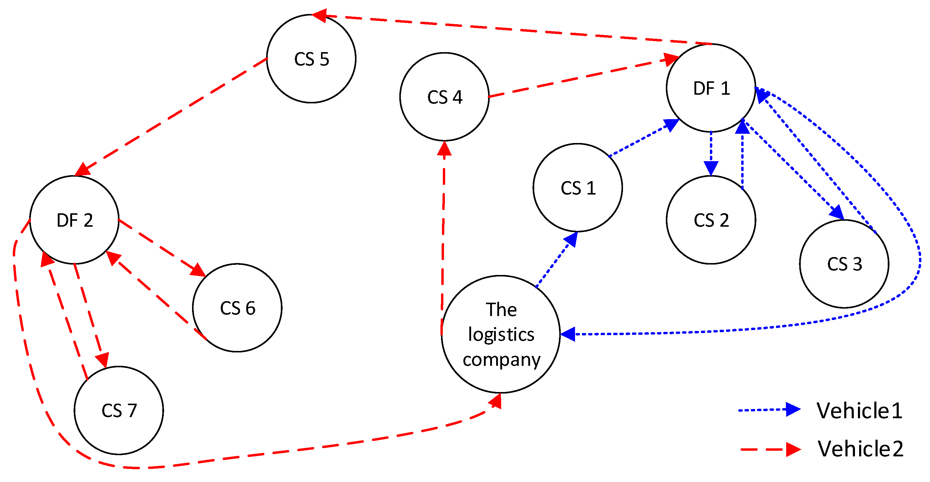
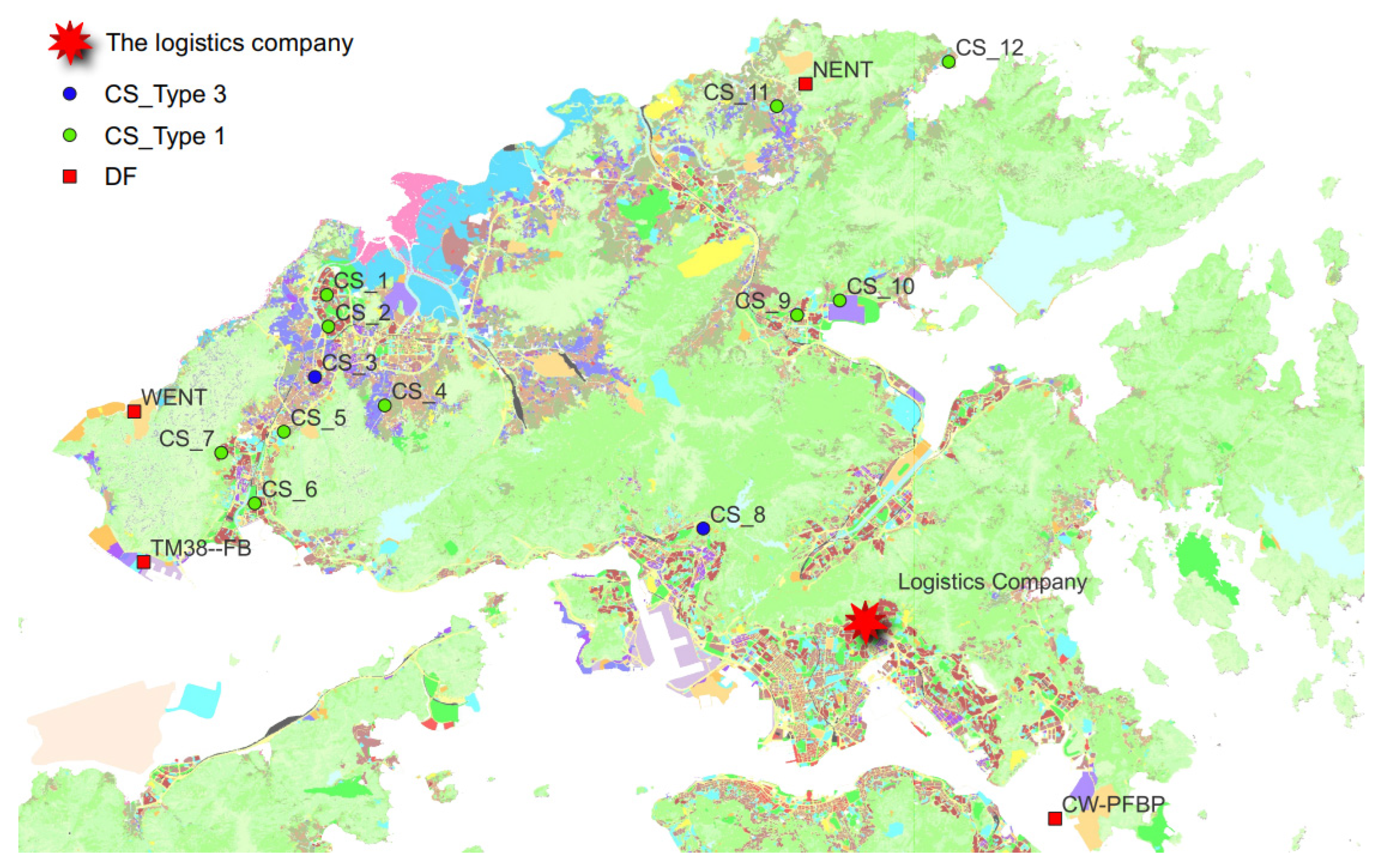
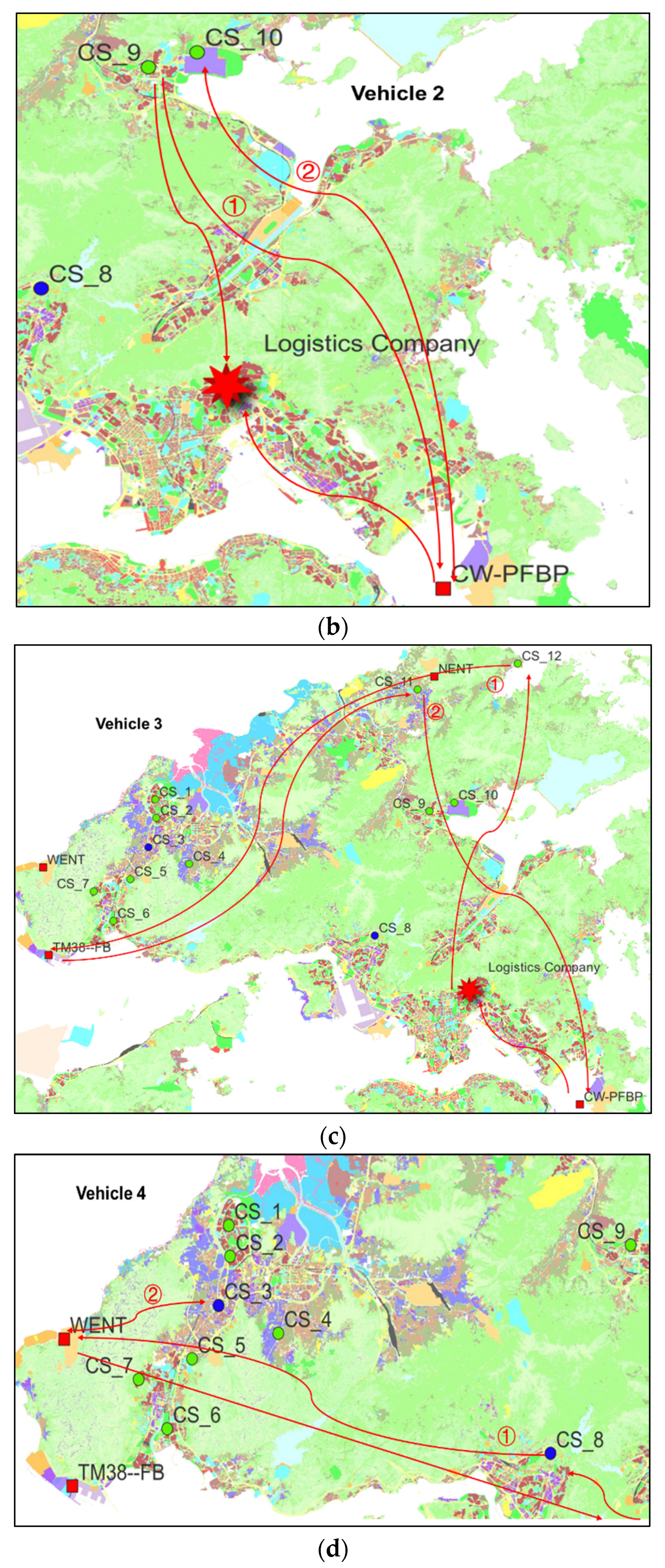
An example of a transportation network is shown in Figure 1. The assigned trucks depart from the logistics company to transport construction waste between the CSs and DFs. Considering the distance and the kind of waste handled by the DFs, one truck may visit different DFs (see Vehicle 2 in Figure 1). Finally, the trucks return to the company from the final DF they visit. Note that in the construction scenario, after a truck transports waste from a CS, it will go to a DF directly and will not go to other CSs for further transportation, so we do not need to consider the load of trucks as long as the capacity of the trucks is large enough to carry the waste from a CS [13]. Furthermore, the aim of our study is to develop a one-day vehicle dispatch schedule, and therefore, the set of CSs that has waste to transport will be different; thus, the model will be re-run, and the vehicle dispatch schedule will be generated and implemented on the next day. In summary, the decision in this transportation system is to choose the optimal service sequence to deliver construction waste at the lowest cost. On the premise that the total waste at each construction site is transported to DFs and the working time of each truck does not exceed 8 h, the overall goal of the transportation system is to minimize the transportation cost (including fixed costs and fuel consumption costs) of the logistics company and the disposal cost that contractors need to pay. The main symbols used in our model are listed in

Table 3. Symbols.

Sets
$K$	Set of DFs, $k\in K$
$J$	Set of CSs, $j\in J$
$S$	Set of trucks, $s\in S$
$J_s$	Set of CSs that truck $s\in S$ can serve
$K_j$	Set of DFs that can handle construction waste from CS $j\in J$
$R_s$	Set of traveling sequence, $r\in R_s$
Parameters
$c_r$	The total cost generated by route r
$c_{jk}$	The cost generated by transporting construction waste from CS j to DF k
$b_{rj}$	Binary variable that equals 1 if route r includes CS j and 0 otherwise
$w$	The loading and unloading time (hour)
$p_{jk}$	The transportation time between CS j and DF k (hour)
$N$	The maximum number of CSs that can be served within one route
Decision Variables
$x_r$	Binary decision variable that equals 1 if route r is chosen and 0 otherwise
$y_{jk}$	Binary decision variable that equals 1 if DF $k\in K_j$ is chosen and 0 otherwise

.

2.1. Integer Programming Model

Consider the system with a single logistics company and multiple CSs and DFs. We use set $J$ to denote the set of CSs and set $K$ to denote the set of DFs. The logistics company has different trucks, denoted by $S$. We use node 0 to denote the logistics company. Different trucks serve different CSs, and we use $J_s$ to denote the CSs that truck $s\in S$ can serve. We use set $K_j$ to denote the DFs that can handle the construction waste from CS $j$. According to $J_s$ and $K_j$, we can enumerate all the traveling sequences of truck $s\in S$. For example, a sequence can be $\left(0,CS1,DF2,CS2,DF2,0\right)$. Note that the first and last node in a sequence must be node 0 and that the CSs and DFs alternate. We define $R_s$ to denote the set of travel sequences $r\in R_s$. The cost generated by route $r$ is denoted by $c_r$, including the transportation cost, fixed cost, and disposal cost. We use the binary variable $b_{rj}$ to indicate whether route $r\in R_s$ visits CS $j$. We use binary decision variable $x_r$ to indicate whether route $r\in R_s$ is selected. Thus, the following integer programming model is formulated:

[M1]

$$\min \sum _{s\in S}\sum _{r\in R_s}{c}_r{x}_r$$

(1)

subject to

$$\sum _{s\in S}\sum _{r\in R_s}{b}_{rj}{x}_r=1,\forall j\in J$$

(2)

$$\sum _{r\in R_s}{x}_r\le 1,\forall s\in S$$

(3)

$$x_r^s\in \left\{0,1\right\},\forall s\in S,r\in R_s$$

(4)

Objective function (1) minimizes the total cost. Constraint (2) indicate that each CS must be visited once, i.e., the construction waste in CSs must be transported. Constraint (3) guarantees that each truck can conduct at most one route per day. Constraint (4) gives the domain of decision variables.

2.2. Generating the Route Space

The key parameter in [M1] is $r\in R_s$. However, $R_s$ could be a very large set if we enumerate all possible routes of truck $s$, resulting in a large number of integer decision variables. For example, if truck $s$ can serve 5 CSs, it will have 325 route sequences in terms of CSs (the number 325 is obtained by calculating the permutations $C_5^1+C_5^2{A}_2^2+C_5^3{A}_3^3+C_5^4{A}_4^4+A_5^5$). The simplest case is that each CS has a unique DF to send its construction waste. If only one CS has two optional DFs, there will be 650 route sequences, and if two CSs each have two optional DFs, there will be 1300 route sequences. We must therefore generate 1300 integer decision variables to choose the optimal route for truck $s$. As the number of DFs increases, the number of permutations increases exponentially. As a result, the efficiency of solving [M1] is greatly reduced. Therefore, the process of generating $R_s$ needs to fully consider the characteristics of the problem to reduce the number of integer decision variables. To simplify notation, we define the following parameters: (1) $w$, the loading and unloading time; (2) $p_{jk}$, the transportation time between CS $j\in J$ and DF $k\in K$; (3) $N$, the maximum number of CSs that can be served within one route sequence. From the problem description, we know that if a truck visits $N$ CSs, it will travel $\left(2N+1\right)$ routes and load and unload $N$ times. We define

$$p_{min}=\min \left\{p_{jk},\forall j\in J,k\in K\right\}$$

(5)

The value of $N$ should satisfy the following formula because the total working time of each truck cannot exceed 8 h per day:

$$\left(2N+1\right)\times p_{min}+w\times N\le 8,\forall j\in J,k\in K$$

(6)

Then the maximum $N$ can be obtained by Equation (7):

$$N=\lfloor \frac{8-p_{min}}{2p_{min}+w}\rfloor$$

(7)

Taking advantage of $N$, we can generate the sequence of CSs with the following Algorithm 1, which contains two typical recursive algorithms for generating combinations and permutations [22]. Note that the sets are converted into arrays in Algorithm 1 for the needs of programming.

Algorithm 1. CSs sequence generating algorithm

Initialize: The maximum number of CSs that can be served by trucks $N\leftarrow \lfloor \frac{8-p_{min}}{2p_{min}+w}\rfloor$

$U_p=\left\{\right\}$//we use $U_p$ to store the generated permutations

$U_c=\left\{\right\}$//we use $U_c$ to store the generated permutations of combinations

//define the function for generating permutations

function Heap ($u$, $U$)

if $u=1$ then

$U_p=U_p\cup U$

else

Heap ($u-1, U$)

for $(v=0, v<u-1, v++$)

if $\left(u\%2\right)=0$ then//determine if n is even or odd

swap $(U\left[v\right]$$, U\left[u-1\right]$)

else

swap $(U\left[0\right]$$, U\left[u-1\right]$)

end if

Heap ($u-1, U$)

end for

end if

return $U_p$

//define the function for generating combinations

function Combination ($U$$, J_s$$, n$)

if $n=0$ then

//now we have the final combination U and then we need to generate permutations based on U

$U_p=\mathbf{Heap} (\mathrm{length}\left(U\right)$$, U$)

$U_c=U_c\cup U_p$

else

for $(i=0, i<\mathrm{length}\left(J_s\right), i++)//\mathrm{length}\left(S\right)$ will count the number of elements in array S

Combination $(U+J_s\left[i\right]$$, S\left[i+1:\right]$$, n-1$)

end for

end if

return $U_c$

$R_s{}^{\prime }=\left\{\right\}$

for$(s=1$$, s\le \mathrm{length}\left(S\right)$$, s++$)

for$(n=1$$, n\le N$$, n++$)

//The input {} means an empty array defined for choosing elements from S according to n

$U_c=$ Combination ($\left\{\right\}$$, J_s$$, n$)

$R_s{}^{\prime }=R_s{}^{\prime }{\cup }^{ }{U}_c$//now we have all the permutations of CSs

end for

end for

for$(s=1$$, s\le \mathrm{length}\left(S\right)$$, s++$)

for $r^{\prime }\in R_s{}^{\prime }$

$\mathrm{Compute} b_{rj}$$, c_r$

end for

for $r^{\prime }\in R_s{}^{\prime }$

if $\mathrm{there} \mathrm{exists} c_{r^{\#}}<c_{r^{\prime }}$$\mathrm{and} \mathrm{elements} \mathrm{in} r^{\prime }=r^{\#}$ then

$\mathrm{drop} r^{\prime }$

end if

end for

Output:$R_s{}^{\prime }$//The permutations of CSs of truck s

Next, we need to insert DF $k\in K$ and node 0 into $r^{\prime }\in R_s{}^{\prime }$ to obtain the final $R_s$. To simplify notation, we define $N_{r^{\prime }}$ to denote the total number of CSs in each $r^{\prime }$ and use $j_{r^{\prime },1},\dots ,j_{r^{\prime },n},\dots ,j_{r^{\prime },N_{r^{\prime }}}$ to denote the sequence ID of CSs in $r^{\prime }$. For example, $r^{\prime }$ could be $\left(CS1,CS3,CS7\right)$, and $j_{r^{\prime },2}$ indicates $CS3$. As our goal is to complete the transportation task at the minimum cost, we can solve [M2-$s$-$r^{\prime }$] for the optimal choice of DFs for each $r^{\prime }\in R_s{}^{\prime }$. The binary decision variable $y_{nk}$ indicates whether DF $k\in K$ is selected to dispose of the waste from CS $j_{r^{\prime },n}$, $n=1,\dots ,N_{r^{\prime }}$. The parameters $c_{j_{r^{\prime },n},k}$ and $t_{j_{r^{\prime },n},k}$ represent the transportation cost and transportation time between CSs and DFs. Parameter $o_k$ represents the disposal cost in DF $k\in K$.

[M2-$s$-$r^{\prime }$]

$$\min {\sum }_{n=1}^{N_{r^{\prime }}-1}{\sum }_{k\in K_{j_{r^{\prime },n}}}\left(c_{j_{r^{\prime },n},k}+c_{k,j_{r^{\prime },n+1}}+o_k\right)y_{nk}+{\sum }_{k\in K_{j_{r^{\prime },N_{r^{\prime }}}}}(c_{j_{r^{\prime },N_{r^{\prime }}},k}+c_{k,0}+o_k)y_{N_{r^{\prime }},k}$$

(8)

subject to

$$\sum _{k\in K_{j_{r^{\prime },n}}}{y}_{nk}=1, n=1,\dots ,N_{r^{\prime }}$$

(9)

$$t_{0,j_{r^{\prime },1}}+\sum _{n=1}^{N_{r^{\prime }}-1}\sum _{k\in K_{j_{r^{\prime },n}}}\left(t_{j_{r^{\prime },n},k}+t_{k,j_{r^{\prime },n+1}}\right)y_{nk}+{\sum }_{k\in j_{r^{\prime },N_{r^{\prime }}}}\left(t_{j_{r^{\prime },N_{r^{\prime }}},k}+t_{k,0}\right)y_{N_{r^{\prime }},k}+N_{r^{\prime }}w\le 8$$

(10)

$$y_{nk}\in \left\{0,1\right\},n=1,\dots ,N_{r^{\prime }},k\in K_{j_{r^{\prime },n}}.$$

(11)

Objective function (8) minimizes the cost of transporting and disposing of construction waste between CS $j_{r^{\prime },n}$, $n=1,\dots ,N_{r^{\prime }}$ and DF $k\in K$ plus the cost of transporting and disposing of construction waste between the final DF and the logistics company (note that we do not consider the cost between the logistics company and the first CS because it does not affect the choice of DF). Constraint (9) restricts that each construction waste in each CS must be transported to one DF. Constraint (10) is the working time limit. Constraint (11) gives the domain of the decision variables. By solving [M2-$s$-$r^{\prime }$], we can obtain the optimal choice of DFs for each route. By solving all the [M2-$s$-$r^{\prime }$] for $r^{\prime }\in R_s{}^{\prime }$, we have the final route space $R_s$.

3. Case Study

3.1. Data

In this section, we conduct a case study based on real CSs and DFs in Hong Kong. The data, including the latitude and longitude of each site, the waste type in each CS, and the names of the DFs, come from Yao et al. [23]. We suppose that the logistics company is located in Kowloon (Hong Kong) and serves CSs within the New Territories (Hong Kong) and Kowloon. We further match the names of DFs with their type according to the public data available from the Hong Kong Environmental Protection Department [14]. As shown in Appendix A, there are two types of DFs within the New Territories and Kowloon. Type 1 indicates public landfill reception facilities that can only handle 100% inert construction waste. Type 3 indicates landfills that can handle construction waste containing a maximum of 50% inert construction waste by weight. As DFs can only dispose of certain types of construction waste, we select CSs that generate type 1 and type 3 construction waste from all the CSs included in Yao et al. [23]. We then randomly pick a point within the area as the logistics company. The geographic coordinates of the CSs and DFs used are shown in Appendix A and Appendix B, respectively. The physical layout of the CSs and DFs is shown in Figure 2.

3.2. Parameter Settings

We first assume that the trucks in the logistics company can serve all of the CSs that generate the same type of construction waste. For example, a truck that can serve CS3 can also serve CS8. The DFs to which the construction waste from each CS can be transported are determined by the DF type and the CS type. For example, the construction waste in CS1 can be sent to DF1 or DF2 (see Appendix A and Appendix B). That is, we have set $J_s$ and $K_j$.

The transportation cost is measured by the real travel distance (km), denoted by $D_{jk}$. According to GOGOVAN [24], the transportation cost equals $\mathrm{USD}\left(4.14+0.33\times D_{jk}\right)$. We set the fixed cost to USD 60, including labor and depreciation costs. Thus, we have $c_{jk}$:

$$c_{jk}=64.14+0.33\times D_{jk},\forall j\in J_s,k\in K_j.$$

(12)

The disposal cost is shown in Table 2. Type 1 DF charges USD 9.05 per ton and Type 3 DF charges USD 25.48 per ton. Note that although the disposal cost varies according to the weight of the construction waste, the optimization results will not be affected by the weight because a certain type of construction waste can only be sent to a DF that disposes of that type of waste, and DFs of the same type charge the same rates.

The transportation time can also be estimated from the real travel distance. We suppose that the average speed of the vehicle is 40 km/h [25]. Then, parameter $p_{jk}$ equals $D_{jk}/40$. The loading and unloading time, i.e., $w$, for each truck is set to 0.5 h. Knowing $p_{jk}$ and $w$, we can calculate the maximum number of served CSs per day.

3.3. Results of Case Study

The results are shown in Figure 3. The company needs to assign four trucks to transport the construction waste generated by these CSs. The four optimal routes are: (Company, CS₄, DF₂, CS₁, DF₂, CS₂, DF₂, CS₅, DF₂, CS₆, DF₂, CS₇, DF₂, Company), (Company, CS₉, DF₁, CS₁₀, DF₁, Company), (Company, CS₁₂, DF₂, CS₁₁, DF₁, Company), and (Company, CS₈, DF₄, CS₃, DF₄, Company). The total transportation cost is USD 423. The working times of vehicles 1, 2, 3, and 4 are 7.8, 4.3, 5.2, and 4.2 h, respectively, and their traveling distances are 189, 201, 181, and 193 km, respectively.

Vehicle 1 serves six CSs that all generate type 1 construction waste and transports all waste to DF₂ (i.e., TM38-FB). We know that the DFs available for Vehicle 1 are DF₁ and DF₂ because Vehicle 1 transports type 1 construction waste. As shown in Figure 2, DF₁ (i.e., CW-PFBP) is located far from these six CSs, and therefore all the construction waste is sent to DF₂ (see Figure 3a). The fixed cost is greater than the transportation cost within a certain distance that is longer than the distance in our optimal solution. Therefore, the optimal solutions should aim to use one vehicle to transport as much construction waste as possible instead of using multiple vehicles. However, Vehicle 1 can only serve these six CSs due to the limit on working hours per day. The type 1 construction waste from both CS₉ and CS₁₀ is transported to DF₁ (i.e., CW-PFBP) considering the transportation cost (see Figure 3b). As shown in Figure 3c, the type 1 construction waste from CS₁₁ and CS₁₂ is transported to DF₂ and DF₁, respectively. However, these four CSs that all generate type 1 construction waste cannot use the same vehicle due to the working time requirement. Finally, there are only two CSs that generate type 3 construction waste, which is sent to DF₄ (i.e., WENT) using one vehicle.

3.4. Computing Performance

To further test the solution efficiency of our proposed method, we randomly generate more CSs (note that the above case study is based on real-world data from Yao et al. [23] and CSs in this subsection are only generated numerically to test the algorithm’s efficiency). In the transportation scenario of construction waste, the number of DFs is usually limited, so we only increase the number of CSs. As in the vehicle routing problem (VRP), studies usually increase the number of customers to test the efficiency of proposed algorithms [26].

The experiments are run on a laptop computer equipped with 2.60 GHz of Intel Core i7 CPU and 16 GB of RAM, and the models are solved using CPLEX Python API 20.1.0. The results are shown in

Table 4. The computing time for different scale instance.

Number of CSs	CPU Time (s)
10	0.75
20	2.08
30	23.32
40	158.28
50	714.53

. The largest instance with 50 CSs can be solved within 12 min, which is efficient enough for practical use as the number of CSs that need to be served is usually not large [27,28]. We also compared our results with other VRP-related studies. For example, Jin and Muriel [26] studied the transportation problem with a single warehouse and multiple retailers. Their largest instance had 50 retailers and was solved within 30 min. Hong [29] explored the vehicle routing problem with time windows, and the largest instance could be solved within 17 min. Although each study has its own problem settings, the computing time of our method is fully acceptable both in theory and in practice.

4. Conclusions

In this paper, we study a construction waste transportation system with a single logistics company and multiple CSs and DFs. Trucks depart from the company at the beginning of a working day to transport construction waste between CSs and DFs. Each truck must go directly to a DF once it is loaded with waste. Different CSs may produce different types of construction waste that must be sent to different DFs. We develop an algorithm to generate the route space in which all routes can meet the working time requirement. With the restriction that all CSs must be served once a day, we propose an integer programming model to decide the optimal routes with the lowest cost. We conduct a case study to show the effectiveness of our model. Our model can provide companies with optimized transportation routes that help to save costs for both the logistics company and contractors. Moreover, as one of the goals of our model is to minimize the transportation cost, designing optimal routes helps to protect the environment by reducing emissions. As a future research direction, we will develop data-driven models that predict the amounts of waste at construction sites and optimize the transportation routes [30,31,32].