Image Reconstruction Algorithm Using Weighted Mean of Ordered-Subsets EM and MART for Computed Tomography

Abstract

Iterative image reconstruction algorithms have considerable advantages over transform methods for computed tomography, but they each have their own drawbacks. In particular, the maximum-likelihood expectation-maximization (MLEM) algorithm reconstructs high-quality images even with noisy projection data, but it is slow. On the other hand, the simultaneous multiplicative algebraic reconstruction technique (SMART) converges faster at early iterations but is susceptible to noise. Here, we construct a novel algorithm that has the advantages of these different iterative schemes by combining ordered-subsets EM (OS-EM) and MART (OS-MART) with weighted geometric or hybrid means. It is theoretically shown that the objective function decreases with every iteration and the amount of decrease is greater than the mean between the decreases for OS-EM and OS-MART. We conducted image reconstruction experiments on simulated phantoms and deduced that our algorithm outperforms OS-EM and OS-MART alone. Our algorithm would be effective in practice since it incorporates OS-EM, which is currently the most popular technique of iterative image reconstruction from noisy measured projections.

1. Introduction

In computed tomography (CT), image reconstruction, an inverse problem of estimating pixel values of a tomographic image from measured projections, is performed in practice by using transform and iterative methods [1,2,3,4,5,6,7]. Iterative image reconstruction [2,5,6,8] algorithms based on the optimization strategy have considerable advantages over transform methods such as the filtered back-projection procedure. Although the maximum-likelihood expectation-maximization (MLEM) [2] algorithm, a well-known iterative method, reconstructs high-quality images even for noisy projection data, it is slow to converge [7,9,10,11]. On the other hand, while the simultaneous multiplicative algebraic reconstruction technique (SMART) [12,13,14,15] converges quickly at early iterations, it is susceptible to noise [16,17].

In this study, we constructed a novel algorithm that has the advantages of these different iterative schemes by combining ordered-subsets versions of MLEM (OS-EM) [7,10] and MART (OS-MART) [14] with a weighted mean. Our method employs combinations of weighted geometric or hybrid means of iterative points. We theoretically show that the objective function for the geometric mean decreases with every iteration and the amount of decrease is greater than the mean between the decreases for OS-EM and OS-MART when the tomographic inverse problem is consistent. By exploiting the complementary advantages of MLEM and SMART, we have created a fast-converging algorithm for reconstructing high-quality images.

Furthermore, we developed a system of switched differential equations with a piecewise smooth vector field, whose numerical discretization corresponds to a combination of the iterative equation for the OS-EM and OS-MART methods. Here, this approach is considered to be an application of the dynamical method [18,19,20,21,22,23] for solving ill-posed inverse problems. The dynamical systems that are applied to constrained tomographic inverse problems [24,25,26,27,28,29] enable us to prove the stability of the equilibrium corresponding to the true image by using the Lyapunov stability theorem [30] and provide a policy for methodically designing a novel algorithm of iterative reconstruction.

A drawback of the weighted-mean iterative algorithm is that a sequential calculation of its terms entails longer computation times per iteration than that of the terms of the individual equation for OS-EM and OS-MART. We show that this issue can be resolved by constructing a fast sequential algorithm with the above discretization scheme for the dynamical system of differential equations. Moreover, we present a time-varying method of improving performance by replacing the constant weight parameter included in the autonomous system with a function of the iteration number.

We conducted numerical experiments on image reconstruction, and the results indicate that our algorithm outperformed OS-EM and OS-MART.

2. Preliminary

The main problem in image reconstruction is to find pixel values $x\in R_{+}^J$ satisfying

$$y=Ax+\delta$$

(1)

where $y\in R_{+}^I$, $A\in R_{+}^{I\times J}$, and $\delta \in R^I$ indicate the projection value, projection operator, and noise, respectively, with $R_{+}$ being the set of nonnegative real numbers. We call the noise-free system in Equation (1) consistent when it has a solution $e\in R_{+}^J$. The tomographic inverse problem of minimizing an objective function can be transformed into one of finding an unknown x, which can be achieved by employing an optimization procedure using either a discrete-time (iterative) or continuous-time system.

The following ideas are related to the ordered-subsets algorithms. Let $A^m\in R_{+}^{I^m\times J}$ be a submatrix consisting of $I^m$ partial rows of A and $y^m\in R_{+}^{I^m}$ be a subvector of y with the same corresponding rows of $A^m$, for $m=1,2,\dots ,M$, with M indicating the total number of divisions.

With $R_{++}$ being the set of positive real numbers, we define the OS-EM algorithm of images $u\left(n\right)\in R_{++}$ as

$$u_j(n+1)=u_j\left(n\right)f_j^m\left(u\left(n\right)\right),u\left(0\right)=z^0\in R_{++}^J$$

(2)

and the OS-MART algorithm of images $v\left(n\right)\in R_{++}$ as

$$v_j(n+1)=v_j\left(n\right)g_j^m\left(v\left(n\right)\right),v\left(0\right)=z^0\in R_{++}^J$$

(3)

for the iteration number $n=0,1,2,\dots ,N-1$ and the subset number $m=(n \mathrm{mod} M)+1$, where

$$f_j^m\left(x\right):=\frac{1}{{\displaystyle \sum _{i=1}^{I^m}{A}_{ij}^m}}\sum _{i=1}^{I^m}{A}_{ij}^m\frac{y_i^m}{{\left(A^{m}x\right)}_i}$$

(4)

and

$$g_j^m\left(x\right):=exp\left({\displaystyle \frac{1}{{\displaystyle \sum _{i=1}^{I^m}{A}_{ij}^m}}\sum _{i=1}^{I^m}{A}_{ij}^{m}log\frac{y_i^m}{{\left(A^{m}x\right)}_i}}\right)$$

(5)

for $j=1,2,\dots ,J$. The iterative solutions $u\left(n\right)$ and $v\left(n\right)$, $n=0,1,2,\dots ,N-1$ for the Equations (2) and (3) remain nonnegative due to the selection of the initial values.

As theoretical measures of convergence, we will use the generalized Kullback–Leibler (KL) divergence [31,32],

$$\mathrm{KL}(\alpha ,\beta ):=\sum _{\ell }{\alpha }_{\ell }log\frac{{\alpha }_{\ell }}{{\beta }_{\ell }}+{\beta }_{\ell }-{\alpha }_{\ell }$$

(6)

for nonnegative vectors $\alpha$ and $\beta$ and the weighted KL-divergence,

$$\mathrm{WKL}(e,x,\Psi ):=\sum _{j=1}^J\mathrm{KL}(e_j,x_j)\sum _{k=1}^K{\Psi }_{kj}$$

(7)

for evaluating $x\in R_{+}^J$ compared with $e\in R_{+}^J$ where $\Psi \in R^{K\times J}$ denotes a projection operator with K rows. The reason why the KL-divergence is used for evaluating the convergence is that it can be considered as an objective function of which there exists a minimizer for each of MLEM and SMART [27,32,33,34].

3. Results

3.1. Proposed Method

Our method of solving the tomographic inverse problem consists of iterative algorithms and dynamical systems.

• Weighted geometric mean:

The iterative reconstruction of an image z involves taking the weighted geometric means of u and v in Equations (2) and (3) with a weight parameter $\alpha \in [0,1]$ and a relaxation or scaling parameter $h>0$:

$$z_j(n+1)=z_j\left(n\right){\left(f_j^m\left(z\left(n\right)\right)\right)}^{h(1-\alpha )}{\left(g_j^m\left(z\left(n\right)\right)\right)}^{h\alpha }$$

(8)

where $z\left(0\right)=z^0\in R_{++}^J$ for $j=1,2,\dots ,J$, $n=0,1,2,\dots ,N-1$, and $m=(n \mathrm{mod} M)+1$. The accompanying system of equations is a continuous analog based on the dynamical method. It is a switched nonlinear system consisting of the following family of M subsystems:

$$\frac{d{x}_j\left(t\right)}{dt}=x_j\left(t\right)\left((1-\alpha )log\left(f_j^m\left(x\left(t\right)\right)\right)+\alpha log\left(g_j^m\left(x\left(t\right)\right)\right)\right)$$

(9)

where the derivative is taken with respect to the state variable $x\left(t\right)$ as an image at $t\in [t^{m-1}+k\tau ,t^m+k\tau )$ with $x\left(0\right)=z^0$ and a sequence of times $0=t^0<t^1<t^2<\cdots <t^M=\tau$, where $k=(n-m+1)/M$ for $j=1,2,\dots ,J$, $n=0,1,2,\dots ,N-1$, and $m=(n \mathrm{mod} M)+1$. It is easy to attain the iterative formula in (8) by using the multiplicative Euler method [35,36] with a step size of h to discretize (9).

• Weighted hybrid mean:

A second pair of discrete- and continuous-time systems can be constructed by making a hybrid combination of additive and multiplicative calculi defined by the iteration,

$$z_j(n+1)=z_j\left(n\right){\left(1+h(1-\alpha )(f_j^m\left(z\left(n\right)\right)-1)\right)}_{+}{\left(g_j^m\left(z\left(n\right)\right)\right)}^{h\alpha },$$

(10)

of images $z\left(n\right)$ with $z\left(0\right)=z^0$, where, for a real number c, ${\left(c\right)}_{+}:=max\{c,0\}$ and its continuous analog:

$$\frac{d{x}_j\left(t\right)}{dt}=x_j\left(t\right)\left((1-\alpha )(f_j^m\left(x\left(t\right)\right)-1)+\alpha log\left(g_j^m\left(x\left(t\right)\right)\right)\right)$$

(11)

of images $x\left(t\right)$ with $x\left(0\right)=z^0$ for $j=1,2,\dots ,J$. The conditions on n, m, t, $t^{\ell }$ for $\ell =0,1,\dots ,M$, $\tau$, and k are the same as in Equations (8) and (9). When $h(1-\alpha )\le 1$, the right-hand side of Equation (10) does not require the clipping operator ${(·)}_{+}$. We can obtain the iterative formula in Equation (10) by discretizing the differential equation in (11). Note that $(f_j^m\left(x\right)-1)$ and $log\left(g_j^m\left(x\right)\right)$ are each zero if and only if $x=e$ holds. The vector field is constructed by adding the terms $(1-\alpha )x_j(f_j^m\left(x\right)-1)$ and $\alpha x_{j}log\left(g_j^m\left(x\right)\right)$, for which additive and multiplicative discretizations using a hybrid Euler method [28] are applied, respectively. The discrete formula in Equation (10) can be regarded as an ordered-subsets version of the iterative reconstruction algorithm [28] derived from an optimization of Jeffreys’ $\alpha$-skew J-divergence [37,38] between the forward and measured projections. Namely, Equation (10) with $M=1$ and $h=\delta$ coincides with Equation (6) in [28].

Notice that each of the iterative Equations (8) and (10) as combinations of weighted geometric and hybrid means reduces to an OS-EM algorithm when $\alpha =0$ and $h=1$ and to the OS-MART algorithm when $\alpha =1$ and $h=1$. A larger value of h in Equations (8) and (10) can accelerate convergence, but the algorithm diverges or oscillates when it is too large. The value of h in our theoretical and experimental results was chosen to be 1 according to the experimental results of OS-EM and OS-MART algorithms as multiplicative Euler discretizations of their continuous analogs [27,34].

3.2. Theoretical Findings

In this section, we present theoretical results on the discrete- and continuous-time systems defined in the previous section under the assumption that the generalized subset balance [33], described as

$$\sum _{i=1}^{I^m}{A}_{ij}^m={\sigma }^m\sum _{i=1}^I{A}_{ij}$$

(12)

for some positive constant ${\sigma }^m$, holds for $m=1,2,\dots ,M$.

• Discrete-time systems:

We consider the discrete-time system in Equation (8) under the assumption $h=1$ and prove that the iterative sequence,

$${\left\{\mathrm{WKL}(e,z(n),A)\right\}}_{n=0}^{\infty }$$

(13)

with $z\left(n\right)\in R_{+}^J$ for $n=0,1,2,\dots$ is decreasing.

Theorem 1.

Let $y=Ae$ for some $e\in R_{++}^J$. Given a solution z to the system in Equation (8) for $h=1$, the inequality,

$$\mathrm{WKL}(e,z\left(0\right),A)-\mathrm{WKL}(e,z\left(1\right),A)\ge \frac{1}{{\sigma }^m}\mathrm{KL}(y^m,A^{m}z\left(0\right)),$$

(14)

is satisfied for any M and $m=1,2,\dots ,M$.

Note that, in Theorem 1 and its proof below, since a discrete time shift has no effect on the autonomous difference system, we have written iteration numbers 0 and 1 instead of n and $n+1$, respectively, for any given $m=1,2,\dots ,M$ with $n=m-1,m,m+1,\dots$, in order to facilitate the description.

Proof 

From the assumption of the generalized subset balance in Equation (12), Inequality (14) is equivalent to

$$\mathrm{WKL}(e,z\left(0\right),A^m)-\mathrm{WKL}(e,z\left(1\right),A^m)\ge \mathrm{KL}(y^m,A^{m}z\left(0\right)).$$

(15)

Let

$$u_j\left(1\right):=u_j\left(0\right)f_j^m\left(u\left(0\right)\right)$$

(16)

and

$$v_j\left(1\right):=v_j\left(0\right)g_j^m\left(v\left(0\right)\right)$$

(17)

for $j=1,2,\dots ,J$, which are one-step updates of the OS-EM and OS-MART equation on the variables u and v with initial values $u\left(0\right)$ and $v\left(0\right)$. Then, we have

$$\mathrm{WKL}(e,z^0,A^m)-\mathrm{WKL}(e,u\left(1\right),A^m)\ge \mathrm{KL}(y^m,A^m{z}^0)$$

(18)

and

$$\mathrm{WKL}(e,z^0,A^m)-\mathrm{WKL}(e,v\left(1\right),A^m)\ge \mathrm{KL}(y^m,A^m{z}^0)$$

(19)

where the initial values $u\left(0\right)$ and $v\left(0\right)$ are the same and equal to $z^0$ (namely, $u\left(0\right)=v\left(0\right)=z^0$). The proof of Inequality (18) is given in [39]. Inequality (19) was first obtained by Byrne [33]. It can also be obtained by applying the procedure of direct reduction [39] using the concavity of the log function and Jensen’s inequality. By multiplying the first and second inequalities by $(1-\alpha )$ and $\alpha$, respectively, and adding the resulting two inequalities side-by-side together, we obtain

$$\begin{array}{ccc}& & \mathrm{WKL}(e,z^0,A^m)-\left((1-\alpha )\mathrm{WKL}(e,u\left(1\right),A^m)+\alpha \mathrm{WKL}(e,v\left(1\right),A^m)\right)\hfill \\ & & \ge \mathrm{KL}(y^m,A^m{z}^0).\hfill \end{array}$$

(20)

Then, the one-step update $z\left(1\right)$ of the algorithm in Equation (8) with $h=1$ and the same initial value,

$$z_j\left(0\right)={\left(u_j\left(0\right)\right)}^{1-\alpha }{\left(v_j\left(0\right)\right)}^{\alpha }=z_j^0,$$

(21)

can be written as

$$z_j\left(1\right)={\left(u_j\left(1\right)\right)}^{1-\alpha }{\left(v_j\left(1\right)\right)}^{\alpha }$$

(22)

for $j=1,2,\dots ,J$. Therefore, we have

$$\begin{array}{ccc}& & \mathrm{WKL}(e,z^0,A^m)-\mathrm{WKL}(e,z\left(1\right),A^m)\hfill \\ & & \ge \mathrm{WKL}(e,z^0,A^m)-\left((1-\alpha )\mathrm{WKL}(e,u\left(1\right),A^m)+\alpha \mathrm{WKL}(e,v\left(1\right),A^m)\right)\hfill \end{array}$$

(23)

according to the following inequality:

$$(1-\alpha )u_j\left(1\right)+\alpha v_j\left(1\right)\ge {\left(u_j\left(1\right)\right)}^{1-\alpha }{\left(v_j\left(1\right)\right)}^{\alpha }$$

(24)

which is in turn derived from Jensen’s inequality,

$$log\left((1-\alpha )\frac{u_j\left(1\right)}{e_j}+\alpha \frac{v_j\left(1\right)}{e_j}\right)\ge (1-\alpha )log\frac{u_j\left(1\right)}{e_j}+\alpha log\frac{v_j\left(1\right)}{e_j}.$$

(25)

The theorem follows directly from inequalities (20) and (23). □

• Continuous-time systems:

When there is no noise and the system in Equation (1) is consistent, we demonstrate that any solution to the continuous analog converges to the wanted solution.

Theorem 2.

Assume there exists $e\in R_{++}^J$ satisfying $y=Ae$. Then, e is an equilibrium for each of the continuous-time systems in Equations (9) and (11) and is asymptotically stable.

Proof 

Notice that e is an equilibrium for each mth subsystem since $f_j^m\left(e\right)=1$ and $g_j^m\left(e\right)=1$ simultaneously hold for $j=0,1,\dots ,J$ and $m=1,2,\dots ,M$. The solutions to the subsystem are in $R_{++}^J$ because the initial state value at $t^{m-1}$, $m=1,2,\dots ,M$, belongs to $R_{++}^J$ and the flow cannot traverse the invariant subspace $x_j=0$ for $j=1,2,\dots ,J$ in the state space. Thus, the following nonnegative function:

$$V\left(x\right):=\mathrm{WKL}(e,x,A)=\sum _{j=1}^J{\int }_{e_j}^{x_j}\frac{w-e_j}{w}dw\sum _{i=1}^I{A}_{ij}$$

of $x_j>0$ is a well-defined common Lyapunov function. Then, we have the derivatives of V along the trajectories of Equations (9) and (11):

$$\begin{array}{ccc}\hfill {\left.\frac{dV}{dt}\left(x\right)\right|}_{\left(9\right)}& =& \sum _{j=1}^J\frac{x_j-e_j}{x_j}\frac{d{x}_j}{dt}\sum _{i=1}^I{A}_{ij}\hfill \\ & =& -(1-\alpha )\sum _{j=1}^J(e_j-x_j)log\left(\frac{1}{{\displaystyle \sum _{i=1}^{I^m}{A}_{ij}^m}}\sum _{i=1}^{I^m}{A}_{ij}^m\frac{y_i^m}{{\left(A^{m}x\right)}_i}\right)\sum _{i=1}^I{A}_{ij}\hfill \\ & & -\frac{\alpha }{{\sigma }^m}\sum _{j=1}^J(e_j-x_j)\sum _{i=1}^{I^m}{A}_{ij}^{m}log\frac{y_i^m}{{\left(A^{m}x\right)}_i}\hfill \\ & \le & -\frac{1-\alpha }{{\sigma }^m}\sum _{i=1}^{I^m}{y}_i^{m}log\frac{y_i^m}{{\left(A^{m}x\right)}_i}\hfill \\ & & +\frac{1-\alpha }{{\sigma }^m}\sum _{i=1}^{I^m}{\left(A^{m}x\right)}_i\left(\frac{y_i^m}{{\left(A^{m}x\right)}_i}-1\right)\hfill \\ & & -\frac{\alpha }{{\sigma }^m}\sum _{i=1}^{I^m}(y_i^m-{\left(A^{m}x\right)}_i)\left(log\left(y_i^m\right)-log\left({\left(A^{m}x\right)}_i\right)\right)\hfill \\ & =& -\frac{1-\alpha }{{\sigma }^m}\mathrm{KL}(y^m,A^{m}x)\hfill \\ & & -\frac{\alpha }{{\sigma }^m}\left(\mathrm{KL}(y^m,A^{m}x)+\mathrm{KL}(A^{m}x,y^m)\right)\hfill \\ & =& -\frac{1}{{\sigma }^m}\left(\mathrm{KL}(y^m,A^{m}x)+\alpha \mathrm{KL}(A^{m}x,y^m)\right)\hfill \\ & \le & 0\hfill \end{array}$$

(26)

and

$$\begin{array}{ccc}\hfill {\left.\frac{dV}{dt}\left(x\right)\right|}_{\left(11\right)}& =& \sum _{j=1}^J\frac{x_j-e_j}{x_j}\frac{d{x}_j}{dt}\sum _{i=1}^I{A}_{ij}\hfill \\ & =& -\frac{1-\alpha }{{\sigma }^m}\sum _{j=1}^J(e_j-x_j)\sum _{i=1}^{I^m}{A}_{ij}^m\left(\frac{y_i^m}{{\left(A^{m}x\right)}_i}-1\right)\hfill \\ & & -\frac{\alpha }{{\sigma }^m}\sum _{j=1}^J(e_j-x_j)\sum _{i=1}^{I^m}{A}_{ij}^{m}log\frac{y_i^m}{{\left(A^{m}x\right)}_i}\hfill \\ & =& -\frac{1-\alpha }{{\sigma }^m}\sum _{i=1}^{I^m}(y_i^m-{\left(A^{m}x\right)}_i)\left(\frac{y_i^m}{{\left(A^{m}x\right)}_i}-1\right)\hfill \\ & & -\frac{\alpha }{{\sigma }^m}\sum _{i=1}^{I^m}(y_i^m-{\left(A^{m}x\right)}_i)\left(log\left(y_i^m\right)-log\left({\left(A^{m}x\right)}_i\right)\right)\hfill \\ & =& -\frac{1-\alpha }{{\sigma }^m}\sum _{i=1}^{I^m}\frac{{\left(y_i^m-{\left(A^{m}x\right)}_i\right)}^2}{{\left(A^{m}x\right)}_i}\hfill \\ & & -\frac{\alpha }{{\sigma }^m}\left(\mathrm{KL}(y^m,A^{m}x)+\mathrm{KL}(A^{m}x,y^m)\right)\hfill \\ & \le & 0.\hfill \end{array}$$

(27)

Therefore, for each system, V is a common Lyapunov function and the equilibrium e is uniformly asymptotically stable. □

The above theorem ensures that the suggested difference system as a first-order approximation to the differential equation has a stable fixed point e when the chosen step size h is small enough to guarantee numerical stability.

3.3. Fast Discretization Algorithm

In Equations (8) and (10), the computational cost of both terms $f_j^m\left(z\right)$ and $g_j^m\left(z\right)$ is higher than that of each single term. Thus, a sequential calculation of the two terms results in a longer computation time. However, because the parts

$$\frac{A_{ij}^m}{{\displaystyle \sum _{i=1}^{I^m}{A}_{ij}^m}}$$

(28)

and

$$\frac{y_i^m}{{\left(A^{m}z\right)}_i}$$

(29)

for $m=1,2,\dots ,M$, $i=1,2,\dots ,I$, and $j=1,2,\dots ,J$ are commonly included in both terms, an effective coding of the program can reduce the computational cost. On the other hand, if approximately the same computation time as OS-EM or OS-MART is required, another method that works by discretizing the continuous-time systems with lower accuracy can be used.

Here, we provide a fast sequential calculation algorithm in the case where $M=1$ and $h=1$, e.g., for the weighted geometric mean:

$$\begin{array}{ccc}\hfill z_j\left(1\right)& =& z_j\left(0\right)p_j\left(0\right) \mathrm{with} \mathrm{calculating} p_j\left(0\right):=f_j\left(z\left(0\right)\right)\mathrm{and} \mathrm{using} \mathrm{an} \mathrm{initial} z_j\left(0\right)=z_j^0\hfill \\ \hfill z_j\left(2\right)& =& z_j\left(1\right){\left(p_j\left(0\right)\right)}^{1-\alpha }{\left(q_j\left(1\right)\right)}^{\alpha }\mathrm{with} \mathrm{calculating} q_j\left(1\right):=g_j\left(z\left(1\right)\right)\mathrm{and} \mathrm{using} p_j\left(0\right)\hfill \\ \hfill z_j\left(3\right)& =& z_j\left(2\right){\left(p_j\left(2\right)\right)}^{1-\alpha }{\left(q_j\left(1\right)\right)}^{\alpha }\mathrm{with} \mathrm{calculating} p_j\left(2\right):=f_j\left(z\left(2\right)\right)\mathrm{and} \mathrm{using} q_j\left(1\right)\hfill \\ \hfill z_j\left(4\right)& =& z_j\left(3\right){\left(p_j\left(2\right)\right)}^{1-\alpha }{\left(q_j\left(3\right)\right)}^{\alpha }\mathrm{with} \mathrm{calculating} q_j\left(3\right):=g_j\left(z\left(3\right)\right)\mathrm{and} \mathrm{using} p_j\left(2\right)\hfill \\ \hfill z_j\left(5\right)& =& z_j\left(4\right){\left(p_j\left(4\right)\right)}^{1-\alpha }{\left(q_j\left(3\right)\right)}^{\alpha }\mathrm{with} \mathrm{calculating} p_j\left(4\right):=f_j\left(z\left(4\right)\right)\mathrm{and} \mathrm{using} q_j\left(3\right)\hfill \\ & ⋮\end{array}$$

for $j=1,2,\dots ,J$ at each step. The vectors p and q whose elements are $p_j$ and $q_j$, respectively, for $j=1,2,\dots ,J$ are calculated alternately. Namely, to calculate the state variable z in the current step, one vector, p or q, is calculated from the previous step and the other is the same one from two steps ago. Although the use of a vector derived from an old state variable leads to a similar effect as having a larger step size and may unstabilize the steady state, the computational cost required for the sequential algorithm is the same as that for either MLEM or SMART. A fast iterative algorithm for the weighted hybrid mean method can be derived in a similar manner by applying the additive and multiplicative terms in Equation (10).

3.4. Time Varying System

In the vector fields of the continuous-time dynamical systems in Equations (9) and (11) with a small value of $\alpha$, the second term $\alpha x_{j}log\left(g_j^m\left(x\right)\right)$ can be considered to be a regularization with which to optimize the metric for OS-MART. When replacing the constant $\alpha$ with a discrete time-varying parameter ${\alpha }_0{\lambda }^n$ where the coefficients ${\alpha }_0$ and $\lambda$ are in the range of 0 to 1, one takes ${\lambda }^n\to 0$, and then the corresponding discretized term $z_j\left(n\right){\left(g_j^m\left(z\left(n\right)\right)\right)}^{{\alpha }_0{\lambda }^n}$ tends to $z_j\left(n\right)$ for $n\to \infty$. The iterative process has the effect of a time-dependent regularization, which makes it possible to optimize dynamically multiple metrics for OS-EM and OS-MART. The discrete time-varying parameter strategy includes the hybrid-cascaded method [40], a two-phased algorithm using the simultaneous algebraic reconstruction technique (SART) as the primary reconstruction to produce an initial estimate for the secondary steps by MLEM, when the constant parameter $\alpha$ is replaced with either 1 if $n\le L$, or 0 otherwise, for a given nonnegative integer L and iteration numbers $n=0,1,2,\dots ,N-1$, although the primary reconstruction method used in [40] is not SMART but rather SART.

4. Experiments and Discussion

We will demonstrate the above-mentioned theory and efficiency of the suggested method by conducting numerical CT experiments. Image reconstructions using combinations of weighted geometric and hybrid means (referred to as GM and HM, respectively) were compared with those of MLEM and SMART. The experiments were conducted using a 3.5 GHz Intel Xeon processor with 96 GB memory and computing tools provided by MATLAB (MathWorks, Natick, MA, USA) without a multi-threading or parallel-processing.

We used a modified Shepp–Logan phantom image composed of $e\in {[0,1]}^J$ and $256\times 256$ pixels ($J=$ 65,536), as shown in Figure 1, and a projection $y\in R_{+}^I$ created by specifying the number of projections and detectors to 360 and 365, respectively ($I=$ 131,400), with 180-degree sampling. The calculation of the forward projection is performed using a highly optimized library for matrix-vector multiplication in MATLAB.

Figure 1. Image of phantom.

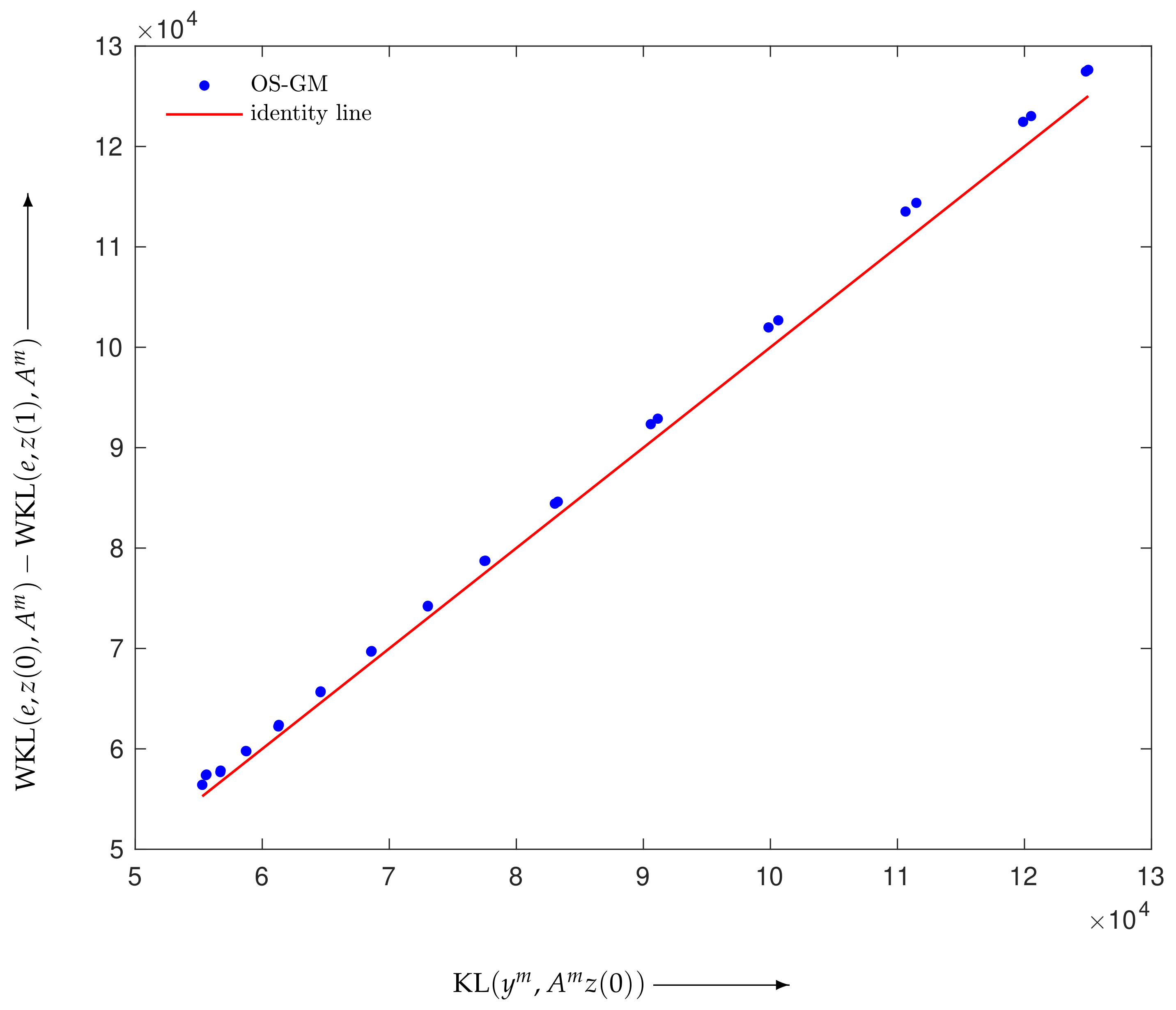
4.1. Verification of Theory

We performed a reconstruction using the weighted geometric mean defined in Equation (8) with $h=1$, $M=30$, $\alpha =0.01$, and a noise-free projection $y=Ae\in R_{+}^I$. An example indicating the validity of Equation (15) is shown in Figure 2, which plots $\mathrm{KL}(y^m,A^{m}z\left(0\right))$ versus $\mathrm{WKL}(e,z\left(0\right),A^m)-\mathrm{WKL}(e,z\left(1\right),A^m)$ applying a one-step iteration $z\left(1\right)$ computed from a given initial state $z\left(0\right)$ through random elements for $m=1,2,\dots ,30$. It can be seen that all the points lie above the line of equality (identity line), as stated in Theorem 1. Another experiment with different values of $\alpha$ yielded similar results.

Figure 2. Scatter plot with the line of equality (red) for OS-GM in Equation (8) with $m=1,2,\dots ,30$.

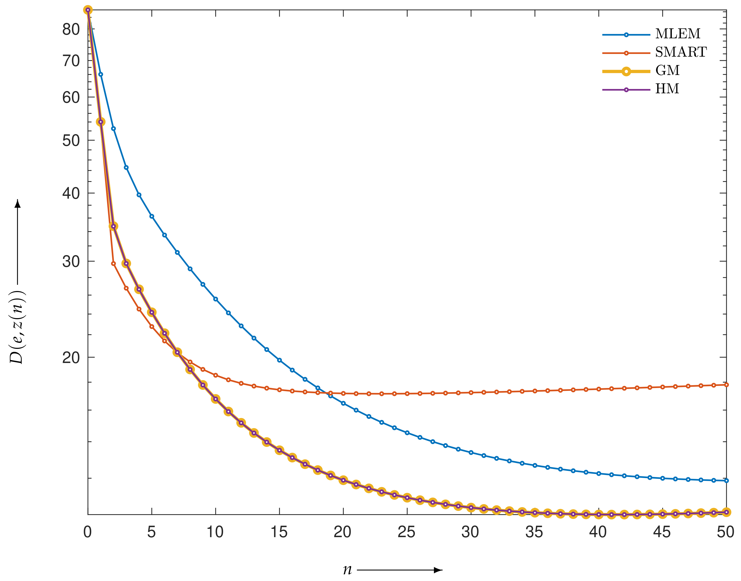
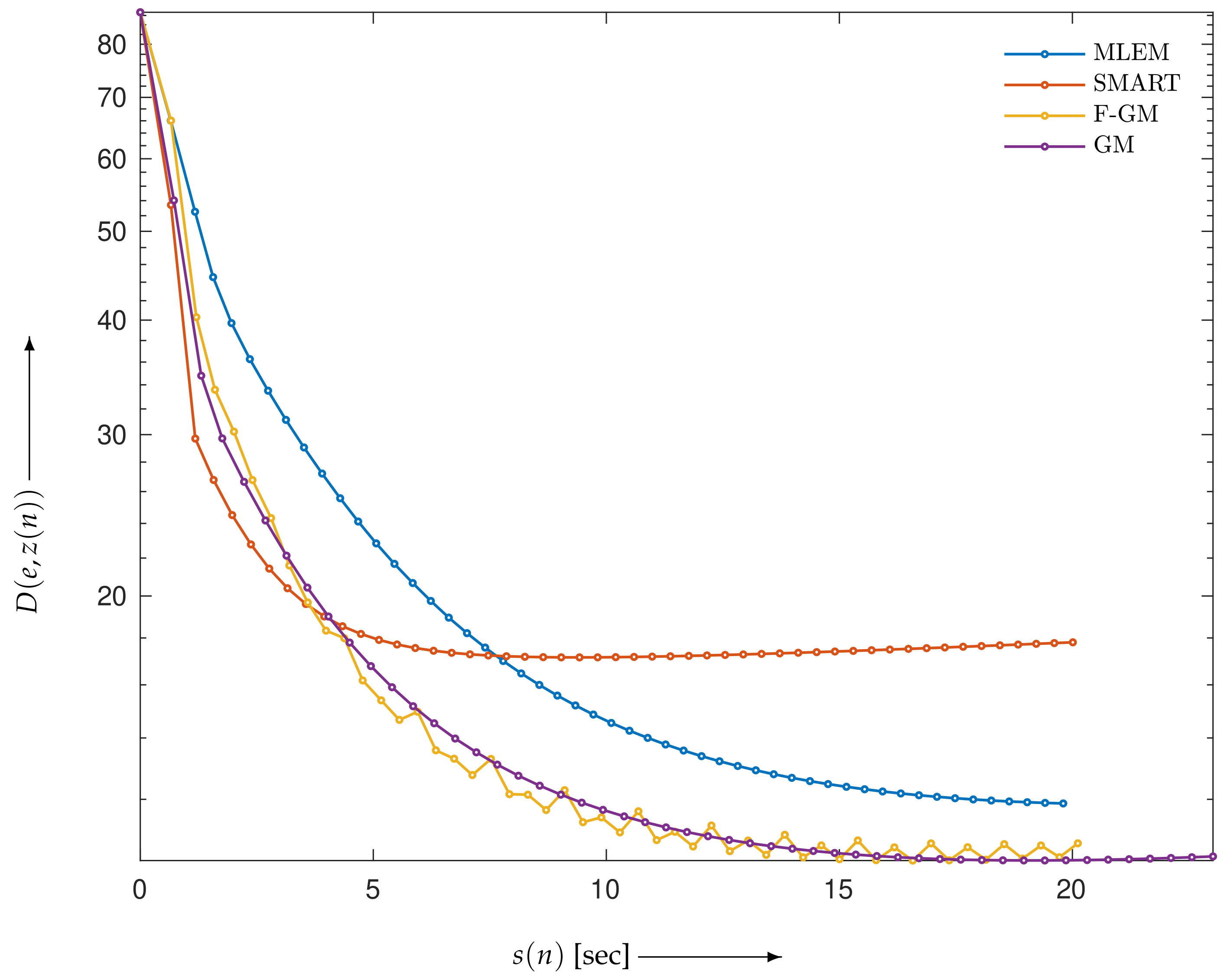
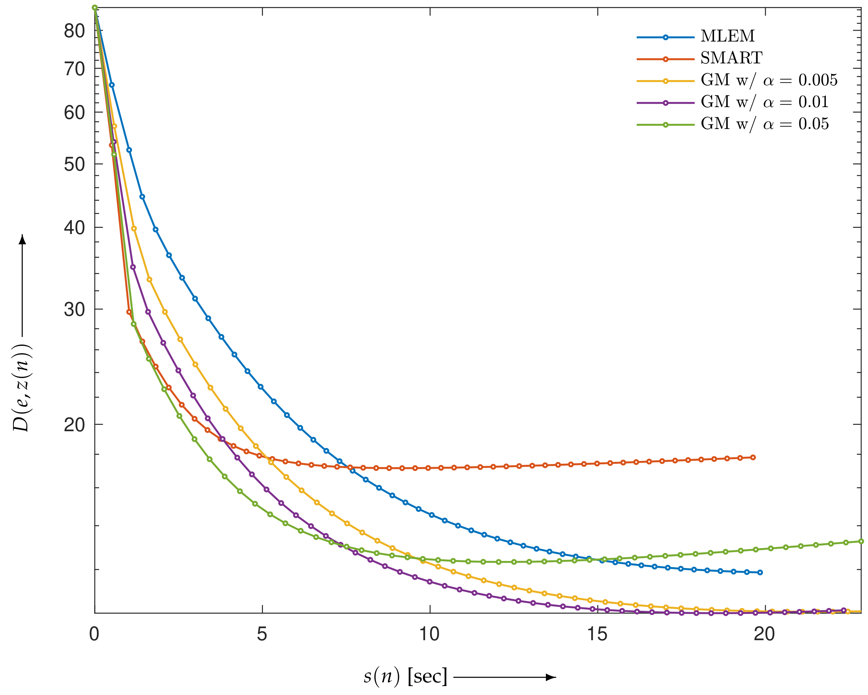
4.2. Evaluation of Reconstructed Images

The noisy projection $y\in R_{+}^I$ obtained from the phantom image was simulated employing Equation (1) with $\delta$ standing for white Gaussian noise so that the signal-to-noise ratio (SNR) was 30 dB unless otherwise specified. We also set a fixed initial value $z_j^0$ for $j=1,2,\dots ,J$ and $h=1$ in Equations (2), (3), (8), and (10). Although putting $h>1$ would hasten convergence, the alteration of h is outside the area of this paper.

To compare the reconstructed image x with the true image e, we defined evaluation functions

$$d_j(e,x):=|e_j-x_j|$$

(30)

for $j=1,2,\dots ,J$ and

$$D(e,x):=\left|\right|e-{x\left|\right|}_2={\left(\sum _{j=1}^J{\left(d_j(e,x)\right)}^2\right)}^{\frac{1}{2}}$$

(31)

which can evaluate the quality of images more directly than $\mathrm{WKL}(e,x,A)$ with weighted coefficients.

Figure 3 displays the evaluation functions $D(e,z(n\left)\right)$ defined in accordance with Equation (31) for the case of $M=1$, $\alpha =0.01$, and noisy projection data for $n=0,1,2,\dots ,50$. Here, we can observe the following. In the early iterations, the SMART algorithm decreases the value of the evaluation function. While the time course of SMART does not exhibit a monotonic decrease, the evaluation function for MLEM monotonically decreases as the number of iterations increases in this range of iterations. It can be seen that the proposed algorithm reduces the evaluation function more than MLEM or SMART.

Figure 3. Evaluation functions for proposed and conventional algorithms at each iteration. The values of the plotted points for GM and HM are almost identical.

Figure 4 graphs the evaluation functions $D(e,z(n\left)\right)$ versus the real computation time $s\left(n\right)$ (in seconds) as a function of the iteration number n for $n=0,1,2,\dots ,50$ under the same settings as in Figure 3. At each iteration of the one-step algorithm, the coefficient in Equation (28) was pre-calculated for all algorithms, and the ratio between the measured and forward projections defined in Equation (29) for each of GM and HM was calculated at every $i=1,2,\dots ,I$. The reconstruction time of the proposed algorithm is approximately 22 s, whereas MLEM and SMART take approximately 20 s in total. Although the proposed algorithm takes 10% longer than the conventional ones, it provides a smaller evaluation function for almost the same computation time ($s\left(43\right)$ for GM or HM) as MLEM or SMART at the 50th iteration. Figure 5 shows images reconstructed by MLEM, SMART, and GM, and the corresponding subtraction images at every pixel, defined as in Equation (30) with $x=u\left(50\right)$, $v\left(50\right)$, and $z\left(43\right)$. The density value of d is on a common scale. By comparing, e.g., the edges of the high-density outer rims in the images, it can be seen that GM generates high-quality reconstructions; this is quantitatively confirmed by the small evaluation function between the phantom and reconstructed images.

Figure 4. Evaluation functions of proposed and conventional algorithms versus computation time for $n=0,1,2,\dots ,50$. The values of the plotted points for GM and HM are almost identical.

Figure 5. Reconstructed images (top plate) and subtraction images (bottom plate) for MLEM and SMART at 50th iteration and for GM at 43rd iteration.

To examine the effectiveness of the sequential discretization algorithm discussed in Section 3.3, we performed reconstructions under the same settings. The time courses of the evaluation functions for MLEM, SMART, GM, and F-GM (short for the fast sequential algorithm using the weighted geometric mean) are plotted in Figure 6 as functions of the computation time. We can see that F-GM has both the same level of performance as GM and the same computational time as MLEM or SMART alone. The oscillatory phenomenon in the iterations that affects F-GM is due to the low accuracy of discretizing the continuous-time system using the state two steps ago. The oscillation can be reduced by choosing the step size h to be less than one in exchange for an increase in computation time, though it is not necessary in this case.

Figure 6. Evaluation functions of proposed and conventional algorithms versus computation time for $n=0,1,2,\dots ,50$.

The proper selection of parameter $\alpha$ is important. As shown in Figure 7, which represents the evaluation functions for GM with $\alpha =0.005$, $0.01$, and $0.05$, $0.01$ provides the best performance. However, Figure 8 shows the effect of changing the SNR of the projections from 30 to 20 dB. Compared with the nonmonotonic decrease in the evaluation function when the SNR is 20 dB and $\alpha$ is $0.05$ (Figure 8), the time-varying system defined in Section 3.4 yields an improvement; for example, by using the exponential function ${\alpha }_0{\lambda }^n$ with coefficients ${\alpha }_0=0.05$ and $\lambda =0.95$ plotted in Figure 9, the values of the evaluation function monotonically decrease up to the 40th iteration. On the other hand, a discontinuous time-varying approach mimicking the hybrid-cascaded method that can be obtained by using SMART in the initial step ($L=0$) and using MLEM in the remaining steps is inferior to the continuous time-varying system (Figure 9). The reason why iterations by the discontinuous time-varying (or MLEM after the second iteration in this case) and pure MLEM algorithms converge to a steady state with the same evaluation function value is conjectured to be that there is a global nonnegative minimizer of an objective function for MLEM.

Figure 7. Evaluation functions of GM for different values of $\alpha$ versus computation time for $n=0,1,2,\dots ,50$.

Figure 8. Evaluation functions of GM using projections with SNR of 20 dB versus computation time for $n=0,1,2,\dots ,50$.

Figure 9. Evaluation functions of proposed and conventional algorithms using projections with SNR of 20 dB at each iteration. $\mathrm{U}$ denotes a unit step function.

The purpose of the next example is to verify the effectiveness of using divided subsets for fixed $\alpha =0.01$. Projections in 180 directions were divided into M nonoverlapping subsets. The ordering of the M subsets was determined using a random projection permutation [41,42]. We can see in Figure 10 that OS-GM with $M=8$ provides better convergence performance with respect to the speed and the evaluation function value compared with not only OS-EM and OS-MART with the same M but also GM and OS-GM with $M=2$. We can also see that, for $M=8$, OS-GM is capable of suppressing the oscillatory phenomenon that appears for successive M iterations in the results of OS-EM. Figure 11 shows images reconstructed by OS-EM with $M=8$ (at the 20th iteration) and GM and OS-GM with $M=8$ (at the 48th and 20th iterations, respectively) and the corresponding subtraction images that were evaluated using the difference from the true image. We can see that OS-GM with $M=8$ provides the best image quality in terms of contrast and artifact.

Figure 10. Evaluation functions for OS-EM, OS-MART, GM, and OS-GM versus computation time for $n=0,1,2,\dots ,N$ along with N equal 60, 45, and 20 for M being 1, 2, and 8, respectively.

Figure 11. Reconstructed images (top plate) and images of subtraction (bottom plate) for GM at 48th iteration and for OS-EM and OS-GM with $M=8$ at 20th iteration.

5. Conclusions

We presented a novel iterative algorithm that combines OS-EM and OS-MART by using weighted geometric or hybrid means. The theoretical results support the convergence of iterative points in view of decreasing of the objective function with increasing of the iteration number. Numerical experiments illustrate that the suggested algorithm and its fast version using a sequential calculation have advantages over the optimization of the evaluation function by MLEM after sufficient iterations as well as by SMART in early iterations. Moreover, our experimental results indicate that the iterative algorithms with a time-varying parameter and the ordered-subsets scheme perform well. In the future, we will use methodologies such as machine learning to make decisions about the best applicable parameter controlled by the numbers of pixels and projections and the noise level of projections, etc.

References

- Ramachandran, G.N.; Lakshminarayanan, A.V. Three-dimensional reconstruction from radiographs and electron micrographs: Application of convolutions instead of Fourier transforms. Proc. Natl. Acad. Sci. USA 1971, 68, 2236–2240. [Google Scholar] [CrossRef] [PubMed]
- Shepp, L.A.; Vardi, Y. Maximum likelihood reconstruction for emission tomography. IEEE Trans. Med. Imaging 1982, 1, 113–122. [Google Scholar] [CrossRef] [PubMed]
- Lewitt, R.M. Reconstruction algorithms: Transform methods. Proc. IEEE 1983, 71, 390–408. [Google Scholar] [CrossRef]
- Natterer, F. Computerized tomography. In The Mathematics of Computerized Tomography; Springer: Berlin/Heidelberg, Germany, 1986; pp. 1–8. [Google Scholar]
- Kak, A.C.; Slaney, M. Principles of Computerized Tomographic Imaging; IEEE Press: Piscataway, NJ, USA, 1988. [Google Scholar]
- Stark, H. Image Recovery: Theory and Application; Academic Press: Washington, DC, USA, 1987. [Google Scholar]
- Hudson, H.M.; Larkin, R.S. Accelerated image reconstruction using ordered subsets of projection data. IEEE Trans. Med. Imaging 1994, 13, 601–609. [Google Scholar] [CrossRef] [PubMed]
- Gordon, R.; Bender, R.; Herman, G.T. Algebraic reconstruction techniques (ART) for three-dimensional electron microscopy and X-ray photography. J. Theor. Biol. 1970, 29, 471–481. [Google Scholar] [CrossRef]
- Fessler, J.A.; Hero, A.O. Penalized maximum-likelihood image reconstruction using space-alternating generalized EM algorithms. IEEE Trans. Image Process. 1995, 4, 1417–1429. [Google Scholar] [CrossRef]
- Byrne, C.L. Accelerating the EMML algorithm and related iterative algorithms by rescaled block-iterative methods. IEEE Trans. Image Process. 1998, 7, 100–109. [Google Scholar] [CrossRef]
- DoSik, H.; Gengsheng, Z.L. Convergence study of an accelerated ML-EM algorithm using bigger step size. Phys. Med. Biol. 2006, 51, 237–252. [Google Scholar]
- Darroch, J.; Ratcliff, D. Generalized iterative scaling for log-linear models. Ann. Math. Stat. 1972, 43, 1470–1480. [Google Scholar] [CrossRef]
- Schmidlin, P. Iterative separation of sections in tomographic scintigrams. J. Nucl. Med. 1972, 11, 1–16. [Google Scholar] [CrossRef]
- Badea, C.; Gordon, R. Experiments with the nonlinear and chaotic behaviour of the multiplicative algebraic reconstruction technique (MART) algorithm for computed tomography. Phys. Med. Biol. 2004, 49, 1455–1474. [Google Scholar] [CrossRef]
- Byrne, C.L. A unified treatment of some iterative algorithms in signal processing and image reconstruction. Inverse Probl. 2004, 20, 103–120. [Google Scholar] [CrossRef]
- Gustavsson, B. Tomographic inversion for ALIS noise and resolution. J. Geophys. Res. Space Phys. 1998, 103, 26621–26632. [Google Scholar] [CrossRef]
- Jiang, W.; Zhang, X. Relaxation Factor Optimization for Common Iterative Algorithms in Optical Computed Tomography. Math. Probl. Eng. 2017, 2017, 4850317. [Google Scholar] [CrossRef]
- Schropp, J. Using dynamical systems methods to solve minimization problems. Appl. Numer. Math. 1995, 18, 321–335. [Google Scholar] [CrossRef]
- Airapetyan, R.G.; Ramm, A.G.; Smirnova, A.B. Continuous analog of gauss-newton method. Math. Model. Methods Appl. Sci. 1999, 9, 463–474. [Google Scholar] [CrossRef]
- Airapetyan, R.G.; Ramm, A.G. Dynamical systems and discrete methods for solving nonlinear ill-posed problems. In Applied Mathematics Reviews; GA, A., Ed.; World Scientific Publishing Company: Singapore, 2000; Volume 1, pp. 491–536. [Google Scholar]
- Airapetyan, R.G.; Ramm, A.G.; Smirnova, A.B. Continuous methods for solving nonlinear ill-posed problems. In Operator Theory and Its Applications; Ramm, A.G., Shivakumar, P.N., Vilgelmovich Strauss, A., Eds.; American Mathematical Society: Providence, RI, USA, 2000; Volume 25, pp. 111–136. [Google Scholar]
- Ramm, A.G. Dynamical systems method for solving operator equations. Commun. Nonlinear Sci. Numer. Simul. 2004, 9, 383–402. [Google Scholar] [CrossRef]
- Li, L.; Han, B. A dynamical system method for solving nonlinear ill-posed problems. Appl. Math. Comput. 2008, 197, 399–406. [Google Scholar] [CrossRef]
- Fujimoto, K.; Abou Al-Ola, O.M.; Yoshinaga, T. Continuous-time image reconstruction using differential equations for computed tomography. Commun. Nonlinear Sci. Numer. Simul. 2010, 15, 1648–1654. [Google Scholar] [CrossRef]
- Abou Al-Ola, O.M.; Fujimoto, K.; Yoshinaga, T. Common Lyapunov function based on Kullback–Leibler divergence for a switched nonlinear system. Math. Probl. Eng. 2011, 2011, 723509. [Google Scholar] [CrossRef]
- Yamaguchi, Y.; Fujimoto, K.; Abou Al-Ola, O.M.; Yoshinaga, T. Continuous-time image reconstruction for binary tomography. Commun. Nonlinear Sci. Numer. Simul. 2013, 18, 2081–2087. [Google Scholar] [CrossRef]
- Tateishi, K.; Yamaguchi, Y.; Abou Al-Ola, O.M.; Yoshinaga, T. Continuous Analog of Accelerated OS-EM Algorithm for Computed Tomography. Math. Probl. Eng. 2017, 2017, 1564123. [Google Scholar] [CrossRef]
- Kasai, R.; Yamaguchi, Y.; Kojima, T.; Yoshinaga, T. Tomographic Image Reconstruction Based on Minimization of Symmetrized Kullback-Leibler Divergence. Math. Probl. Eng. 2018, 2018, 8973131. [Google Scholar] [CrossRef]
- Kasai, R.; Yamaguchi, Y.; Kojima, T.; Abou Al-Ola, O.M.; Yoshinaga, T. Noise-Robust Image Reconstruction Based on Minimizing Extended Class of Power-Divergence Measures. Entropy 2021, 23, 1005. [Google Scholar] [CrossRef] [PubMed]
- Lyapunov, A.M. Stability of Motion; Academic Press: New York, NY, USA, 1966. [Google Scholar]
- Kullback, S.; Leibler, R.A. On information and sufficiency. Ann. Math. Stat. 1951, 22, 79–86. [Google Scholar] [CrossRef]
- Byrne, C.L. Iterative image reconstruction algorithms based on cross-entropy minimization. IEEE Trans. Image Process. 1993, 2, 96–103. [Google Scholar] [CrossRef]
- Byrne, C.L. Block-iterative algorithms. Int. Trans. Oper. Res. 2009, 16, 427–463. [Google Scholar] [CrossRef]
- Tateishi, K.; Yamaguchi, Y.; Abou Al-Ola, O.M.; Kojima, T.; Yoshinaga, T. Continuous analog of multiplicative algebraic reconstruction technique for computed tomography. In Proceedings of the SPIE, Medical Imaging 2016; SPIE Medical Imaging: San Diego, CA, USA, 2016; Volume 9783-4Q. [Google Scholar]
- Aniszewska, D. Multiplicative Runge–Kutta methods. Nonlinear Dyn. 2007, 50, 265–272. [Google Scholar] [CrossRef]
- Bashirov, A.E.; Kurpinar, E.M.; Oezyapici, A. Multiplicative calculus and its applications. J. Math. Anal. Appl. 2008, 337, 36–48. [Google Scholar] [CrossRef]
- Jeffreys, H. Theory of Probability; Clarendon Press: Oxford, UK, 1939. [Google Scholar]
- Jeffreys, H. An invariant form for the prior probability in estimation problems. R. Soc. Lond. 1946, 186, 453–461. [Google Scholar]
- Ishikawa, K.; Yamaguchi, Y.; Abou Al-Ola, O.M.; Kojima, T.; Yoshinaga, T. Block-Iterative Reconstruction from Dynamically Selected Sparse Projection Views Using Extended Power-Divergence Measure. Entropy 2022, 24, 740. [Google Scholar] [CrossRef]
- Tiwari, S.; Srivastava, R. A Hybrid-Cascaded Iterative Framework for Positron Emission Tomography and Single-Photon Emission Computed Tomography Image Reconstruction. J. Med. Imaging Health Inform. 2016, 6, 1001–1012. [Google Scholar] [CrossRef]
- Kazantsev, I.G.; Matej, S.; Lewitt, R.M. Optimal Ordering of Projections using Permutation Matrices and Angles between Projection Subspaces. Electron. Notes Discret. Math. 2005, 20, 205–216. [Google Scholar] [CrossRef]
- Van Dijke, M.C. Iterative Methods in Image Reconstruction. Ph.D. Thesis, Rijksuniversiteit Utrecht, Utrecht, The Netherlands, 1992. [Google Scholar]
Publisher’s Note: MDPI stays neutral with regard to jurisdictional claims in published maps and institutional affiliations. |
© 2022 by the authors. Licensee MDPI, Basel, Switzerland. This article is an open access article distributed under the terms and conditions of the Creative Commons Attribution (CC BY) license (https://creativecommons.org/licenses/by/4.0/).