Abstract
High-order harmonic generation (HHG), the nonlinear upconversion of coherent radiation resulting from the interaction of a strong and short laser pulse with atoms, molecules and solids, represents one of the most prominent examples of laser–matter interaction. In solid HHG, the characteristics of the generated coherent radiation are dominated by the band structure of the material, which configures one of the key properties of semiconductors and dielectrics. Here, we combine an all-optical method and deep learning to reconstruct the band structure of semiconductors. Our method builds up an artificial neural network based on the sensitivity of the HHG spectrum to the carrier-envelope phase (CEP) of a few-cycle pulse. We analyze the accuracy of the band structure reconstruction depending on the predicted parameters and propose a prelearning method to solve the problem of the low accuracy of some parameters. Once the network is trained with the mapping between the CEP-dependent HHG and the band structure, we can directly predict it from experimental HHG spectra. Our scheme provides an innovative way to study the structural properties of new materials.
MSC:
81Q05; 68T07
1. Introduction
The energy band structure is an important characteristic to describe the properties of a crystal. The usual way to map the band structure is to use a technique called angle-resolved photo emission spectroscopy (ARPES), where the momentum and the energy of incoherent emitted electrons are measured independently [1]. ARPES is based on the photoelectric effect proposed by Einstein—electrons in a material will escape by absorbing the energy of a photon under the interaction with light and the maximum kinetic energy of the electron is then , where is the photon energy and is the work function of the material. ARPES is generally used to reconstruct the band structure of 2D materials, such as graphene and high-temperature superconductors. However, it is typically challenging to detect and correctly characterize the emitted photoelectrons, mainly due to the influence of the ambient conditions [2]. The band structure can also be calculated from “first principles”, i.e., by solving the time independent Schrödinger equation (TISE) directly. One of the the most well-known and used software packages is the Vienna AB-Initio Simulation Package (VASP). However, VASP calculations generally require a large number of empirical parameters, which limits its application into the field of new materials [3,4,5,6].
High-order harmonic generation (HHG) is one of the most important phenomena resulting from the nonlinear interaction between strong laser fields and matter (atoms, molecules and recently solids). HHG has been widely used to generate attosecond pulses. These ultrashort sources of coherent radiation allow one to follow the ultrafast electron dynamics in real time [7,8]. The study of solid HHG has received a boost since the first experimental measurement of HHG in ZnO crystals by S. Ghimire et al. [9,10] in 2011. In 2014, Vampa et al. [11] proposed a model for solid HHG based on the well-known atomic three-step model [12], which shed light on the underlying generation mechanisms. The solid three-step model can be described as follows: (i) an electron tunnels vertically from the valence to the conduction band, (ii) the laser subsequently accelerates the electron–hole pair within the bands (intraband acceleration) and (iii) the electron recombines with the hole and emits a harmonic photon (interband transition). Since these electron dynamics are significantly affected by the band structure and band gap energy, both leave fingerprints in the solid HHG spectrum and play an instrumental role in determining the properties of the emitted high-order harmonics. In recent years, several all-optical methods have been proposed based on the solid HHG. In 2015, G. Vampa et al. [13] proposed a technique to reconstruct the momentum-dependent band gaps by exploiting the coherent motion of the electron–hole pairs driven by intense mid-infrared femtosecond laser pulses. However, the biggest limitation of this method is that the even-order harmonics are difficult to capture because of their weak intensity, so the reconstruction of the band gap in the high-energy region is not very accurate. Typically, due to the symmetry properties of both the solid material and driven laser field, only odd-order harmonics are generated. In 2020, Liang Li et al. [14] proposed a method to reconstruct the band structure of semiconductors based on a temporal Young’s interferometer. Here, a few-cycle laser pulse was used to generate the high-order harmonics in the solid. The strict requirements about the number of cycles of the driven laser pulse made this method difficult to implement experimentally.
Concurrently, machine learning (ML) has been a very fruitful platform to tackle a plethora of problems within the physical sciences [15,16,17,18,19,20]. These problems mainly emerge from nonlinear systems, which indicates that ML could present clear advantages compared with traditional methods. Here, we propose a method combining a new all-optical method with ML to reconstruct the semiconductor band structure. Specifically, we exploit the strong sensitivity of solid HHG to the CEP of a few-cycle laser pulse. The CEP-dependent features in the HHG spectrum make up a nonlinear mapping with the band structure of the material. This allows us to use this mapping to train our neural network. With the well-trained neural network, we are able to successfully predict the band gap of the target solid with the measured CEP-dependent harmonic spectrum. Our result shows that it is completely feasible to reconstruct the band structure through ML, thus providing a new scheme for exploring the fundamental physical properties of new materials, combining strong field laser–matter processes and ML.
This article is divided into the following parts: The second section introduces the generation and processing of the input data, as well as the construction of the ML model. Next, we discuss the validity of the model and accuracy of the predicted results. Finally, we briefly summarize our work. We also include some technical details in Appendix A.
2. Methods
2.1. Data Generation and Preprocessing
Reasonable feature selection plays an important role in learning the mapping relationship between the input and output [21,22,23]. The shape of an individual HHG spectrum seems to be the most straightforward choice, but it is inevitably affected by the difference between experimental and theoretical calculations, particularly, the instability of the experimental waveform due to the influence of experimental conditions. In other words, the experimental and theoretical HHG spectra differ for a same system and same band. In this case, even though we can train adequately the model and reconstruct the target band structure with the calculated data, it is difficult to obtain the band information by experimental HHG data. Furthermore, the shape of the laser pulse has a strong modulation effect on HHG. In particular, for few-cycle and subcycle pulses, the change of the carrier-envelope phase (CEP) can have a large impact on HHG features, which enables, for instance, attosecond dynamical imaging in atoms, molecules and solids with the hallmarks of attosecond optical spectroscopy [24,25,26,27,28,29,30,31]. Recently, it was demonstrated in MgO that the experimentally measured harmonic spectrum showed a strong CEP-dependent shift [27]. In our previous paper, we demonstrated that this CEP-dependent shift originated in the interference between adjacent harmonics. Subsequently, this property was confirmed and adopted to measure the CEP of a few-cycle laser pulse [32,33]. Here, we further show that this CEP-dependent shift can be used as a new all-optical probing method to reconstruct the band structure.
Figure 1a shows the numerically calculated CEP dependence of HHG from magnesium oxide (MgO) along the direction. The band structure used for the calculation was obtained from a multicosine fit with the same parameters as reported in Ref. [34]. The HHG spectra were computed by using the semiconductor Bloch equation (SBE) (see Appendix A for more details). In order to verify the accuracy of the numerical calculation, we chose the same laser field as in Ref. [27] and compared the CEP dependence of HHG with the experimental results. A two-cycle full width at half-maximum (FWHM) laser pulse with a peak laser electric field of was used. The numerical calculations had an excellent agreement with the experimental results reported in [27]. A relatively weak field strength was used to ensure the applicability of the two-band model [35,36,37]. Meanwhile, a moderate laser intensity is typically required in order to operate below the damage threshold of the material [38,39]. In the following, we use this CEP-dependent spectrum as the test data set, and the corresponding adopted band structure as the target to text the applicability of the trained neural network.
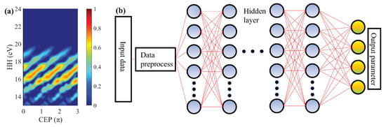
Figure 1.
(a) CEP dependence of HHG from MgO calculated by the SBE. The theoretical calculations reproduce very well the experimental results presented in [27]. For a better comparison with the experimental data, a laser with field strength of and excitation carrier wave central wavelength of , corresponding to a laser period was used. In the numerical simulations, a Gaussian shaped envelope with FWHM was adopted. MgO band was calculated by Equation (1) with , , and , respectively. (b) Schematic illustration of the multilayer perceptron (MLP) used in our investigations.
The training data set was obtained by numerical solution of the semiclassical SBE with different band structure parameters. We used a general polynomial expansion to describe the band structure, which can be view as an approximation of that obtained from an ab initio approach,
where is the Bloch wavevector of the lattice and a is the lattice constant of the material. In Equation (1), are the random parameters for various bands. To obtain the training data set, are randomly chosen within certain ranges. Here, represents the minimum band gap. In order to avoid the singularity caused at the Dirac points, we set . This value contains the band gap range for a vast majority of semiconductor materials. The other three parameters were set to , . The range of values of shows that metals were not included in the learned samples. One important reason was that it was not clear how the nonlinear response would be and if a high-order harmonic spectrum would show up in normal metals due to the zero band gap. Interestingly, it was recently demonstrated that it was possible to generate high-order harmonics in a high-Tc superconductor [40] and that the HHG spectrum was sensitive to the different phases (strange metal, pseudo gap and superconductor). Here, to ensure the robustness of the model, we did not consider metals, but, in principle, our scheme could be applied in such materials. Figure 2 shows the energy bands and the corresponding CEP-dependent spectrum with different parameters of with the same laser parameters. It can be seen that the CEP-dependent spectrum including the cutoff and the shift depended sensitively on the band structures. These band structure data did not correspond to some specific material but could provide us training data from which the mapping relationship between the specific properties of the CEP-dependent harmonic spectrum and the band structure parameters could be learned by the neural network. We calculated a total of 12,000 samples, of which 8500 served as the training set, and the remaining ones were used as the test set. It should be noticed that the target data, which the theoretical simulation reproduced well with the “MgO experiment”, was not included in the training sample so as to prove the portability of the neural network. In order to be consistent with the experimental results in harmonic yield intensities, we normalized each HHG sample individually. We also locally averaged and normalized each sample before they were entered as input data into the model to reduce the quantity of data as well as to facilitate the learning.
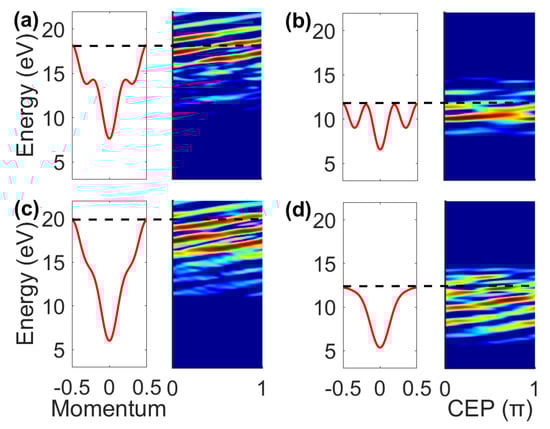
Figure 2.
Panels (a–d) show four CEP-dependent HHG spectra and the corresponding band gaps, randomly generated. The black dashed lines show the HHG cutoff, linked to the high-energy region of the band gap. Every HHG spectrum shares the same colorbar with a normalized intensity. All the panels confirm the strong influence of the band gap shape on the HHG, especially for the high-energy region.
2.2. Model Structure
Machine learning (ML) has developed rapidly in recent years. In order to deal with various problems, people have put forward a variety of network models, such as convolutional neural networks for image classification and object detection [41,42], recurrent neural networks for speech recognition [43], generative adversarial networks for super-resolution and optimization problems [44,45], amongst others. In physics, the common problem, regression problem, seems easy to solve by multilayer perceptrons (MLPs), also called feed-forward neural networks [18,19,46,47]. Figure 1b shows a brief sketch of an artificial neural network (ANN). Here, we used an MLP with six fully connected (FC) layers, excluding the input and output layers. Each FC layer had 200 neurons and an hyperbolic tangent (tanh) activation function was adopted to increase the nonlinearity of the model. The random CEP-dependent HHG spectra shown in Figure 2, which were converted to a one-dimensional array with 350 elements, were the inputs, and the corresponding band gap parameters including the 4 elements were the outputs of the NN. The weights were initialized by the method mentioned in Ref. [48], which could significantly increase the convergence speed of the model. The mean square error (MSE) was adopted as the loss function, which is defined as:
Here, m is the number of samples and n is the number of parameters. and are the predicted and true value, respectively.
3. Results
Figure 3a shows the training and testing loss as a function of the number of steps. Both curves decreased rapidly at the beginning of the training process and then saturated at a low value. To evaluate the accuracy of the model more intuitively, we considered as an accurate predictor sample, and defined , with the number of accurate predicted sample for the ith parameter and the number of total predicted samples, as the precision rate. From Figure 3b–e, we can clearly see that the accuracy of , the band gap, was the highest. In contrast, and had the lowest accuracy. This behavior can be understood as follows. It can be seen from Equation (1) that has the largest impact on the band since its coefficient is always equal to one, which means that it also will have a larger influence on the HHG spectra compared to the rest of the parameters, which is always less than one since their coefficients are functions. In this way, the network can identify and learn more straightforwardly. However, the rest of the parameters have less influence on the band shape, and, as a consequence, on the HHG. This makes their learning much more difficult. We find that even increasing the numbers of the layer and the neurons of each layer, it is difficult to get a high accuracy for all the four parameters at the same time.
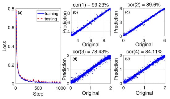
Figure 3.
(a) The loss of the training and testing processes. Both training and testing losses converge to a very small value rapidly at the beginning of the training process. (b–e) show the precision rate of four band parameters, respectively. We can see that , the band gap, has the highest accuracy.
To improve the accuracy in the estimation of and make the model more robust, we proposed a solution called prelearning method. Specifically, after training the model, we put the input data we wanted to predict (i.e., the CEP-dependent HHG) into the model as prelearning data to get the target band gap parameters. Since was the parameter with the highest prediction accuracy and played a decisive role in the energy band, we only kept the predicted , while we let the neutral network relearn with the training data, thus was kept as the predicted one, while the other three parameters were randomly chosen. Figure 4a shows the precision rate of the parameters variation with the sample size adopted in the relearning process. Here, we can observe that the precision rate was improved for the three parameters. It also shows that the number of samples required to reach a precision rate of in the predicted parameters was much smaller than in the previous training. The precision rate could be improved by more than when the number of samples was about 4500.
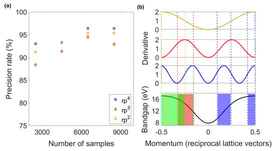
Figure 4.
(a) Variation of the precision rate for with the number of training samples. (b) From top to bottom, the derivatives of the band gap with respect to and the band gap are shown, respectively. The colored area shows where each of the three parameters makes a major contribution to the band. For easier presentation, only the left or right half of each component contribution is displayed.
Based on the above method, we put the “experimental input data” mentioned above into two models to obtain the prediction results, as shown in Figure 5. Figure 5a shows the predicted band gap from training once (red dashed line) with the predicted , , and , respectively. Figure 5b shows the predicted band gap from the prelearning method (red dashed line) which was , , and , respectively. For comparison, we show the target band gap with which the SBE simulation reproduces well the experimental result with a blue line. From comparing the differences in Figure 5 or the parameter values, it is easy to see that the prelearning method predicts the band gap more accurately, especially for the high-energy part.
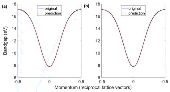
Figure 5.
(a) Comparison of the predicted band gap from training once (red dashed line) with the desired (blue solid line) MgO band gap. (b) Result for prelearning method with 4500 input samples (red dashed line) and the desired MgO band gap (blue solid line).
It is important to note that our training and testing samples, including the MgO sample above, were formed by samples of the identical and independent distribution (IID). This means that the discussion of accuracy and error in our work is within the parameters of the sample. Although we chose a parameter range to take into account the majority of semiconductor band gaps as much as possible, for some band gaps (e.g., semiconductors with very large band gaps), the errors may be large. Limited by the availability of experimental data, we did not consider the accuracy of samples outside the parameter range for at the time. Recently, X. Ma et al. [49] discussed this issue and optimized the model by controlling the parameter range, which provides a possible route to solve this problem and extend the applicability of our model.
4. Discussion
Reexamining Figure 4a, we can reveal that regardless of the number of samples, always had the lowest precision rate, which was in contrast to the fact that the precision rate of was always the highest. To analyze the underlying reason, we then performed an analysis of the contribution of these three parameters to the band, as shown in Figure 4b, which is the derivative of the band gap with respect to the parameters. Compared with , and had a greater impact on the high-energy region of the band, that is, near the boundary of the BZ. It is well-known that the third step of the three-step model (recombination), plays an instrumental role on the HHG cutoff. This means that changes in and will have more influence in the HHG spectra, making them easier to learn for the model, and thus obtaining a higher precision rate. It is also the reason why had the highest precision rate as seen in Figure 3. On the contrary, the HHG hardly depended on . Consequently, here we obtained a low precision rate. It is hard to distinguish the individual influence of and on the energy band and HHG, but we still can infer that was easier to learn. We can then conclude that it is related to its impact on the characteristics of the HHG in the plateau region.
This phenomenon demonstrates that indeed the physical models do have an impact on the result of ML. For regression models with multiple output parameters, different parameters contribute to different degrees to the input features, which can cause a distinct learning accuracy (even considering data processing features such as normalization). The greater the influence on the input features, the more accurate the learning, and conversely, i.e., the smaller the impact, the more inaccurate the learning is, regardless of the ML model itself. The proof of this phenomenon seems complicated, which is closer to exploring the underlying details of ML (see Ref. [50] for a similar discussion about this).
5. Conclusions
In conclusion, we provided a solution for reconstructing the energy band of semiconductors. To overcome the low accuracy of some parameters, we proposed a prelearning method to solve it, which greatly improved the accuracy of the predicted parameters. Finally, we were able to predict the energy band from the experimentally measured HHG. The method did not need too much prior knowledge of the material to complete the whole modeling process. Our approach thus provided an attractive perspective to study the structure of novel materials using an all-optical ultrafast technique. In principle, the driving laser itself does not have any effect on the energy band structure and only initiates an electron–hole dynamic. Because of the ultrashort time range (sub-fs) of the recollision electron–hole pair process, all-optical band structure measurement inherently has an ultrafast temporal resolution. Thus, not only is it possible to reach a picometer spatial resolution but also a sub-fs temporal resolution, allowing the tracking of the laser-initiated processes in real time [51]. Yet, our approach could be extended to other related phenomena. For instance, the effect of the waveguides on the bands of photonic crystals was recently studied [52,53]. Since our model is based on the nonlinear effect of the strong laser field interacting with matter and without considering the propagation process, it is not suitable to apply our approach under such conditions directly. However, one can use the mapping between a given observable and one (or more) input parameters to develop a similar method to ours. The feasibility of such an implementation will be dictated by the sensitivity of the output signal with the input quantities, i.e., the larger the change, the higher the probability to reconstruct the material properties using an ML scheme.
Author Contributions
Conceptualization, W.Y.; methodology, S.Y., Xiwang Liu; software, S.Y. and J.L.; validation, X.S.; formal analysis, R.Z.; investigation, S.Y.; resources, S.Y.; data curation, S.Y.; writing—original draft preparation, S.Y.; writing—review and editing, X.S., M.C. and W.Y.; visualization, S.Y.; supervision, X.S.; project administration, W.Y.; funding acquisition, X.S., M.C. and W.Y. All authors have read and agreed to the published version of the manuscript.
Funding
This research was supported by the National Natural Science Foundation of China (grants nos. 91950101, 12074240, 12264013, 12204135 and 12204136), Hainan Provincial Natural Science Foundation of China (grant nos. 122CXTD504 and 122QN217) and Sino-German Mobility Programme (grant no. M-0031). M.C. acknowledges financial support from the Guangdong Province Science and Technology Major Project (Future functional materials under extreme conditions-2021B0301030005).
Institutional Review Board Statement
Not applicable.
Informed Consent Statement
Not applicable.
Data Availability Statement
The data that support the findings of this study are available from the corresponding author, upon reasonable request.
Conflicts of Interest
The authors declare no conflict of interest.
Appendix A. Numerical Method for Solving HHG: Semiconductor Bloch Equation
A two-band semiconductor Bloch equation (SBE) can be derived from the time-dependent Schrödinger equation (TDSE) and expressed as [11,54,55,56,57]:
Here, and are the interband polarization and the occupation of electrons (holes), respectively. is the electron’s crystal momentum with the initial momentum and the laser vector potential , where is the laser electric field. Here, is the ionization time of the electron, is the recombination time of the electron-hole pair () and is the dephasing time. is called the Rabi frequency, with the dipole matrix element. is the classical action, where is the k-dependent transition band gap between the valence and conduction bands.
The final emitted radiation can be determined by the macroscopic current , due to the intraband motion, and the macroscopic polarization , caused by the interband light emission contribution, which are given, respectively, by:
and
where is called the band velocity. The HHG spectrum can be obtained from the Fourier transform (FT) of the total emitted radiation, . Only the interband contribution was considered in our calculations, the intraband HHG being negligible for the laser parameters used in our work (see, e.g., [11,14] for more details).
Our work focused on the semiconductor band gap rather than the specific band structure. This was indeed related to the underlying mechanism behind the HHG process. It can be seen from the Equations (A1) and (A2) that the mapping we established was the CEP dependence of the HHG with the band gap rather than to the band structure itself. In fact, it was demonstrated that higher bands were active as well, when the laser electric field strength increased. Here, a multiplateau structure in the HHG showed up [29,58]. However, even if more bands were involved in the HHG process, it would be the band gap between the different bands the parameter that would play the instrumental role [59].
References
- Damascelli, A.; Hussain, Z.; Shen, Z.X. Angle-resolved photoemission studies of the cuprate superconductors. Rev. Mod. Phys. 2003, 75, 473. [Google Scholar] [CrossRef]
- Shuvaev, A.M.; Dziom, V.; Mikhailov, N.N.; Kvon, Z.D.; Shao, Y.; Basov, D.N.; Pimenov, A. Band structure of a two-dimensional Dirac semimetal from cyclotron resonance. Phys. Rev. B 2017, 96, 155434. [Google Scholar] [CrossRef]
- Kresse, G.; Hafner, J. Ab initio molecular dynamics for liquid metals. Phys. Rev. B 1993, 47, 558. [Google Scholar] [CrossRef] [PubMed]
- Kresse, G.; Hafner, J. Ab initio molecular-dynamics simulation of the liquid-metal–Amorphous-semiconductor transition in germanium. Phys. Rev. B 1993, 49, 14251. [Google Scholar] [CrossRef]
- Kresse, G.; Furthmüller, J. Efficiency of ab initio total energy calculations for metals and semiconductors using a plane-wave basis set. Comput. Mater. Sci. 1996, 6, 15. [Google Scholar] [CrossRef]
- Kresse, G.; Furthmüller, J. Efficient iterative schemes for ab initio total-energy calculations using a plane-wave basis set. Phys. Rev. B 1996, 54, 11169. [Google Scholar] [CrossRef]
- Corkum, P.; Krausz, F. Attosecond science. Nat. Phys. 2007, 3, 381–387. [Google Scholar] [CrossRef]
- Krausz, F.; Ivanov, M. Attosecond physics. Rev. Mod. Phys. 2009, 81, 163. [Google Scholar] [CrossRef]
- Shambhu, G.; Di Chiara, A.D.; Emily, S.; Pierre, A.; DiMauro, L.F.; David, A.R. Observation of high-order harmonic generation in a bulk crystal. Nat. Phys. 2011, 7, 138–141. [Google Scholar]
- Park, J.; Subramani, A.; Kim, S.; Ciappina, M.F. Recent trends in high-order harmonic generation in solids. Adv. Phys.-X 2022, 7, 2003244. [Google Scholar] [CrossRef]
- Vampa, G.; McDonald, C.R.; Orlando, G.; Klug, D.D.; Corkum, P.B.; Brabec, T. Theoretical Analysis of High-Harmonic Generation in Solids. Phys. Rev. Lett. 2014, 113, 073901. [Google Scholar] [CrossRef] [PubMed]
- Corkum, P.B. Plasma perspective on strong field multiphoton ionization. Phys. Rev. Lett. 1993, 71, 1994. [Google Scholar] [CrossRef] [PubMed]
- Vampa, G.; Hammond, T.J.; Thiré, N.; Schmidt, B.E.; Légaré, F.; McDonald, C.R.; Brabec, T.; Klug, D.D.; Corkum, P.B. All-Optical Reconstruction of Crystal Band Structure. Phys. Rev. Lett. 2015, 115, 193603. [Google Scholar] [CrossRef] [PubMed]
- Li, L.; Lan, P.F.; He, L.X.; Cao, W.; Zhang, Q.B.; Lu, P.X. Determination of Electron Band Structure using Temporal Interferometry. Phys. Rev. Lett. 2020, 124, 157403. [Google Scholar] [CrossRef]
- Mills, K.; Spanner, M.; Tamblyn, I. Deep learning and the Schrödinger equation. Phys. Rev. A 2017, 96, 042113. [Google Scholar] [CrossRef]
- Zahavy, T.; Dikopoltsev, A.; Moss, D.; Haham, G.; Cohen, O.; Mannor, S.; Segev, M. Deep learning reconstruction of ultrashort pulses. Optica 2018, 5, 666. [Google Scholar] [CrossRef]
- Ryczko, K.; Strubbe, D.A.; Tamblyn, I. Deep learning and density-functional theory. Phys. Rev. Lett. 2019, 100, 022512. [Google Scholar] [CrossRef]
- Liu, X.W.; Zhang, G.J.; Li, J.; Shi, G.L.; Zhou, M.Y.; Huang, B.Q.; Tang, Y.J.; Song, X.H.; Yang, W.F. Deep Learning for Feynman’s Path Integral in Strong-Field Time-Dependent Dynamics. Phys. Rev. Lett. 2020, 124, 113202. [Google Scholar] [CrossRef]
- Kirkpatrick, J.; McMorrow, B.; Turban, D.H.P.; Gaunt, A.L.; Spencer, J.S.; Matthews, A.G.D.G.; Obika, A.; Thiry, L.; Fortunato, M.; Pfau, D.; et al. Pushing the frontiers of density functionals by solving the fractional electron problem. Science 2021, 374, 1385–1389. [Google Scholar] [CrossRef]
- Shvetsov-Shilovski, N.I.; Lein, M. Deep learning for retrieval of the internuclear distance in a molecule from interference patterns in photoelectron momentum distributions. Phys. Rev. A 2022, 105, L021102. [Google Scholar] [CrossRef]
- Li, Y.; Li, T.; Liu, H. Recent advances in feature selection and its applications. J. Mach. Learn. Res. 2010, 9, 249–256. [Google Scholar] [CrossRef]
- Li, J.D.; Cheng, K.W.; Wang, S.H.; Morstatter, F.; Trevino, R.; Tang, J.L.; Liu, H. Feature Selection: A Data Perspective. ACM Comput. Surv. 2018, 50, 1–45. [Google Scholar] [CrossRef]
- Cai, J.; Luo, J.W.; Wang, S.L.; Yang, S. Feature selection in machine learning: A new perspective. Neurocomputing 2018, 300, 70–79. [Google Scholar] [CrossRef]
- Smirnova, O.; Mairesse, Y.; Patchkovskii, S.; Dudovich, N.; Villeneuve, D.; Corkum, P.; Ivanov, M.Y. High harmonic interferometry of multi-electron dynamics in molecules. Nature 2009, 460, 972–977. [Google Scholar] [CrossRef]
- Hohenleutner, M.; Langer, F.; Schubert, O.; Knorr, M.; Huttner, U.; Koch, S.W.; Kira, M.; Huber, R. Real-time observation of interfering crystal electrons in high-harmonic generation. Nature 2015, 523, 572–575. [Google Scholar] [CrossRef]
- Silva, R.E.F.; Jiménez-Galán, Á.; Amorim, B.; Smirnova, O.; Ivanov, M. Topological strong-field physics on sub-laser-cycle timescale. Nat. Photonics 2019, 13, 849–854. [Google Scholar] [CrossRef]
- You, Y.S.; Wu, M.X.; Yin, Y.C.; Chew, A.; Ren, X.M.; Gholam-Mirzaei, S.; Browne, D.A.; Chini, M.; Chang, Z.H.; Schafer, K.J.; et al. Laser waveform control of extreme ultraviolet high harmonics from solids. Opt. Lett. 2017, 42, 1816–1819. [Google Scholar] [CrossRef]
- Hawkins, P.G.; Ivanov, M.Y. Role of subcycle transition dynamics in high-order-harmonic generation in periodic structures. Phys. Rev. A 2013, 87, 063842. [Google Scholar] [CrossRef]
- Guan, Z.; Zhou, X.X.; Bian, X.B. High-order-harmonic generation from periodic potentials driven by few-cycle laser pulses. Phys. Rev. A 2016, 93, 033852. [Google Scholar] [CrossRef]
- Yang, W.F.; Lin, Y.C.; Chen, X.Y.; Xu, Y.X.; Zhang, H.D.; Ciappina, M.; Song, X.H. Wave mixing and high-harmonic generation enhancement by a two-color field driven dielectric metasurface. Chin. Opt. Lett. 2021, 19, 123202. [Google Scholar] [CrossRef]
- Zhang, H.D.; Liu, X.W.; Zhu, M.; Yang, S.D.; Dong, W.H.; Song, X.H.; Yang, W.F. High-order-harmonic generation from periodic potentials driven by few-cycle laser pulses. Chin. Phys. Lett. 2021, 38, 063201. [Google Scholar] [CrossRef]
- Song, X.H.; Zuo, R.X.; Yang, S.D.; Li, P.C.; Meier, T.; Yang, W.F. Attosecond temporal confinement of interband excitation by intraband motion. Opt. Express 2019, 27, 2225–2234. [Google Scholar] [CrossRef] [PubMed]
- Hollinger, R.; Paulus, G.G.; Wustelt, P.; Skruszewicz, S.; Zhang, Y.; Kang, H.; Würzler, D.; Jungnickel, T.; Dumergue, M.; Nayak, A.; et al. Carrier-envelope-phase measurement of few-cycle mid-infrared laser pulses using high harmonic generation in ZnO. Opt. Express 2020, 28, 7314. [Google Scholar] [CrossRef] [PubMed]
- Vampa, G.; Lu, J.; You, Y.S.; Baykusheva, D.R.; Wu, M.X.; Liu, H.Z.; Schafer, K.J.; Gaarde, M.B.; Reis, D.A.; Ghimire, S. Attosecond synchronization of extreme ultraviolet high harmonics from crystals. Optica 2020, 53, 144003. [Google Scholar] [CrossRef]
- McDonald, C.R.; Vampa, G.; Corkum, P.B.; Brabec, T. Interband Bloch oscillation mechanism for high-harmonic generation in semiconductor crystals. Phys. Rev. A 2015, 92, 033845. [Google Scholar] [CrossRef]
- Wu, M.X.; Ghimire, S.; Reis, D.A.; Schafer, K.J.; Gaarde, M.B. High-harmonic generation from Bloch electrons in solids. Phys. Rev. A 2015, 91, 043839. [Google Scholar] [CrossRef]
- Lanin, A.A.; Stepanov, E.A.; Fedotov, A.B.; Zheltikov, A.M. Mapping the electron band structure by intraband high-harmonic generation in solids. Optica 2017, 4, 516–519. [Google Scholar] [CrossRef]
- Uzan, A.J.; Orenstein, G.; Jiménez-Galán, Á. Attosecond spectral singularities in solid-state high-harmonic generation. Nat. Photonics 2020, 16, 183–187. [Google Scholar] [CrossRef]
- Nourbakhsh, Z.; Tancogne-Dejean, N.; JiMerdji, H.; Rubio, A. High Harmonics and Isolated Attosecond Pulses from MgO. Phys. Rev. A 2021, 16, 014013. [Google Scholar] [CrossRef]
- Alcalà, J.; Bhattacharya, U.; Biegert, J.; Ciappina, M.; Elu, U.; Graß, T.; Grochowski, P.T.; Lewenstein, M.; Palau, A.; Sidiropoulos, T.P.H.; et al. High-harmonic spectroscopy of quantum phase transitions in a high-Tc superconductor. Proc. Natl. Acad. Sci. USA 2022, 119, e2207766119. [Google Scholar] [CrossRef]
- Shin, H.C.; Roth, H.R.; Gao, M.C.; Lu, L.; Xu, Z.Y.; Nogues, I.; Yao, J.H.; Mollura, D.; Summers, R.M. Deep Convolutional Neural Networks for Computer-Aided Detection: CNN Architectures, Dataset Characteristics and Transfer Learning. IEEE Trans. Med. Imaging 2016, 35, 1285–1298. [Google Scholar] [CrossRef] [PubMed]
- Ren, S.; He, K.; Girshick, R.; Sun, J. Faster R-CNN: Towards Real-Time Object Detection with Region Proposal Networks. IEEE Trans. Pattern Anal. Mach. Intell. 2017, 39, 1137–1149. [Google Scholar] [CrossRef] [PubMed]
- Yu, Y.; Si, X.; Hu, C.; Zhang, J. A Review of Recurrent Neural Networks: LSTM Cells and Network Architectures. Neural Comput. 2019, 31, 1235–1270. [Google Scholar] [CrossRef] [PubMed]
- Creswell, A.; White, T.; Dumoulin, V.; Arulkumaran, K.; Sengupta, B.; Bharath, A.A. Generative Adversarial Networks: An Overview. IEEE Signal Process. Mag. 2018, 35, 53–65. [Google Scholar] [CrossRef]
- Goodfellow, I.J.; Pouget-Abadie, J.; Mirza, M.; Xu, B.; Warde-Farley, D.; Ozair, S.; Courville, A.C.; Bengio, Y. Generative Adversarial Nets. NIPS 2018, 2, 2672–2680. [Google Scholar]
- Raissia, M.; Perdikarisb, P.; Karniadakisa, G.E. Physics-informed neural networks: A deep learning framework for solving forward and inverse problems involving nonlinear partial differential equations. J. Comput. Phys. 2019, 378, 686–707. [Google Scholar] [CrossRef]
- Gherman, A.M.M.; Kovács, K.; Cristea, M.V.; Tosa, V. Artificial Neural Network Trained to Predict High-Harmonic Flux. Appl. Sci. 2018, 8, 2106. [Google Scholar]
- Glorot, X.; Bengio, Y. Understanding the difficulty of training deep feedforward neural networks. J. Mach. Learn. Res. 2010, 9, 249–256. [Google Scholar]
- Ma, X.R.; Tu, Z.C.; Ran, S.J. Deep Learning Quantum States for Hamiltonian Estimation. Chin. Phys. Lett. 2021, 38, 110301. [Google Scholar]
- Li, C.; Huang, H.P. Learning Credit Assignment. Phys. Rev. Lett. 2020, 125, 178301. [Google Scholar] [CrossRef]
- Luu, T.T.; Garg, M.; Kruchinin, S.Y.; Moulet, A.; Hassan, M.T.; Goulielmakis, E. Extreme ultraviolet high-harmonic spectroscopy of solids. Nature 2015, 521, 498–502. [Google Scholar] [CrossRef] [PubMed]
- Díaz-Escobar, E.; Mercadé, L.; Barreda, Á.I.; García-Rupérez, J.; Martínez, A. Photonic Bandgap Closure and Metamaterial Behavior in 1D Periodic Chains of High-Index Nanobricks. Photonics 2022, 9, 691. [Google Scholar] [CrossRef]
- Sirmaci, Y.; Gomez, A.B.; Pertsch, T.; Schmid, J.; Cheben, P.; Staude, I. All-Dielectric Huygens’ Meta-Waveguides for Resonant Integrated Photonics, PREPRINT (Version 1) Available at Research Square. Available online: https://www.researchsquare.com/article/rs-1929644/v1 (accessed on 5 October 2022).
- Golde, D.; Meier, T.; Koch, S.W. High harmonics generated in semiconductor nanostructures by the coupled dynamics of optical inter- and intraband excitations. Phys. Rev. B 2008, 77, 075330. [Google Scholar] [CrossRef]
- McDonald, C.R.; Vampa, G.; Corkum, P.B.; Brabec, T. Intense-Laser Solid State Physics: Unraveling the Difference between Semiconductors and Dielectrics. Phys. Rev. Lett. 2017, 118, 173601. [Google Scholar] [CrossRef] [PubMed]
- Song, X.H.; Yang, S.D.; Zuo, R.X.; Meier, T.; Yang, W.F. Enhanced high-order harmonic generation in semiconductors by excitation with multicolor pulses. Phys. Rev. A. 2020, 101, 033410. [Google Scholar] [CrossRef]
- Zuo, R.X.; Trautmann, A.; Wang, G.F.; Hannes, W.R.; Yang, S.D.; Song, X.H.; Meier, T.; Ciappina, M.; Duc, H.T.; Yang, W.F. Neighboring Atom Collisions in Solid-State High Harmonic Generation. Ultrafast Sci. 2021, 9861923. [Google Scholar] [CrossRef]
- Liu, X.; Zhu, X.S.; Lan, P.F.; Zhang, X.F.; Wang, D.; Zhang, Q.B.; Lu, P.X. Time-dependent population imaging for high-order-harmonic generation in solids. Phys. Rev. A 2017, 95, 063419. [Google Scholar] [CrossRef]
- Luu, T.T.; Wörner, H.J. High-order harmonic generation in solids: A unifying approach. Phys. Rev. B 2016, 94, 115164. [Google Scholar] [CrossRef]
Publisher’s Note: MDPI stays neutral with regard to jurisdictional claims in published maps and institutional affiliations. |
© 2022 by the authors. Licensee MDPI, Basel, Switzerland. This article is an open access article distributed under the terms and conditions of the Creative Commons Attribution (CC BY) license (https://creativecommons.org/licenses/by/4.0/).