Kinematic Modes Identification and Its Intelligent Control of Micro-Nano Particle Manipulated by Acoustic Signal

Abstract

In this paper, the dynamics of a micro-nano particle on the micro-thin plate driven by an acoustic signal was investigated, including the particle kinematics mode, kinematics equation, and trajectory control. According to Newton’s kinematic theorem, analyzing the forces acting on the particle, the kinematic modes of the driven particle are distinguished with specific mathematical conditions, which are classified as slide, bounce, and stable modes strictly planned on a thin plate area. Based on the theory of kinematic modal analysis, the simulation results reveal the distribution rules of particle motion modes against the driving signal or plate geometry. The particle kinematics equation governing the sliding movement on the thin plate was then derived in light of the interaction between the particle and driving signal, based on which, the particle trajectory was drawn and analyzed in detail. For the purpose of controlling the particle trajectory, the control problem was designed in accordance with a linear active disturbance rejection controller (LADRC). Further, a guidance law was proposed, and the corresponding controller was designed to realize the linear trajectory following.

1. Introduction

Over the years, micro-nano manipulation methods have been continuously explored and studied, among which, mainstream technologies include optical tweezers [1,2,3,4], electromagnetic manipulation [5,6], acoustic manipulation, such as the acoustic subwavelength manipulation of particles using a quasiperiodic plate in [7], the control of multiple objects on a Chladni plate [8], the manipulation of objects in two dimensions using a single transducer acoustic levitator [9], and the rotational manipulation of single cells and organisms, which is achieved using acoustic waves [10]. Each manipulation mode has its own characteristics and advantages. For example, mature optical tweezers technology has been widely used in manufacturing; electromagnetic manipulation focuses on the control of particles with electromagnetic properties; acoustic manipulation has unique advantages due to its non-contact control, long wavelength range and good environmental compatibility [11,12,13]. For the theories and applications of acoustic manipulation methods, there is still a big gap that needs to be filled, which contains particle surface dynamics, particle kinematic control and the extension of application scenarios.

Expectedly, the technology of acoustic manipulation is broadly applied in the biomedical field, high-performance material processing, chip-based manufacture, particle shaping, particle trajectory tracking and particle separation [14,15,16]. The acoustic manipulation process indispensably needs the acoustic signal driver and media manipulation needs a metal thin plate, which can be traced back to 1787, when the Chladni effect was discovered [17,18,19,20]. It is described as a metal sheet placed on a violin, where sand was sprinkled evenly on it. Playing the violin with the bow results in the sand being automatically arranged into different beautiful patterns. With different tunes and an increasing frequency of the strings, the patterns also changed and became more complex. Therefore, the movement of particles on a forced vibrating thin plate can be realized by changing the frequency, amplitude and other parameters of the acoustic signal. Some related findings have been reported, such as the Chladni effect, which is used to control the motion of multiple micro-objects in [8]; the controlled manipulation and active sorting of particles inside microfluidic chips, which are realized using bulk acoustic waves in [13]; the use of acoustic waves to rotate single cells and organisms in [21]; the implementation of the acoustic manipulation of cells and microbeads in droplet microfluidics [22]; the use of three sound waves to produce a standing wave field that realizes two-dimensional acoustic manipulation [23]. On the other hand, investigating how many ways there are for particles to generate displacement on the forced vibration plate and how to determine the motion mode of particles in each area of the thin plate is the key to achieving the control tasks.

Particle surface dynamics is governed by the vibrating thin plate so that particles on the surface of the thin plate can visualize the sound signal [24]. The kinematics of particles can be described by components of the deflection function of the forced vibration thin plate in each direction of motion [25,26]. When studying the particle kinematics, Newton’s second law of particles in horizontal and vertical directions should be analyzed. Additionally, the static friction between the particle and thin plate must be considered [27]; otherwise, the sliding motion of particles on the thin plate cannot be discussed. The maximum static friction will be a critical value used to distinguish whether particles slide or jump to generate displacement on the sheet. According to the conclusion of the Chladni effect, there must be some areas characterized by the particles that remain in their original positions [28,29]. In this regard, different kinematic modes can be distinguished in the thin plate area. Furthermore, particles in fixing modes cannot produce displacement; the kinematics of particle jumping is too complex to control; on the sliding region of the thin plate, the control equation of particle kinematics can be derived. In this paper, a square silicon thin plate driven by an acoustic signal is discussed. Different motion modes of particles on the thin plate were distinguished by theoretical analysis and numerical simulation, the dynamic motion model of particles in the gliding region was deduced, and its trajectory was also solved and analyzed.

When the particle is located on the sliding region of the driven plate, the particle will move under the control of Newton’s equation of kinematics. In this way, the velocity and direction of particle motion will be uncontrolled [30,31,32]. In particular, the movement will be influenced by the initial conditions, excitation time, and driving acoustic signal. In this case, the particle motion is beyond control. For this reason, the intelligent control algorithm should be applied to control and improve particle motion. In this work, LADRC was used to achieve the particle tracking following. LADRC has the advantages of strong robustness, a large controllable range, a simple algorithm, and easy implementation in engineering, and it directly establishes the error relation between the input and output and regards the equivalent total output affecting the output as the total disturbance, which was real-time estimated using an extended state observer and suppressed [33,34,35]. According to the algorithm mechanism of LADRC, the path following the control of the particle on the sliding region of the thin plate was formulated.

The rest of this paper is arranged as the following: in Section 2, using Newtonian kinematics and the theory of thin plate vibration, mathematical conditions for different particle modes on the thin plate surface are accurately depicted, and a simulation is also carried out. In Section 3, we discuss the dynamics of the particle, the kinematics governing the equation of particles in gliding mode is derived, and its movement characteristics are analyzed. Particle tracking control for linear trajectory is performed in Section 4 based on LADRC, which explains the control mechanism and displays the simulation results. Lastly, conclusions and future work are stated in Section 5.

2. Particle Kinematic Modes

Acoustic wave manipulation technology provides an effective means of micro-nano target control. The actual system studied is shown in Figure 1, from which, the square micro-thin plate is horizontally fixed on the piezoelectric actuator. The particle to be manipulated is placed on the surface of the thin plate. A sine signal is sent from the computer and applied to the actuator. During the excitation, how does the particle move on the plate? Analyzing and mastering its kinematic modes contribute to the application of the platform.

2.1. Identification of The Modes

Usually, the particle motions on the forced vibrating plate can be assumed as bounce, slide, and fixed, respectively. When the square thin plate is excited by an ideal central sound source, the vibration of the plate is governed by the following equation:

$$\rho h\frac{{\partial }^{2}w}{\partial t^2}+D{\nabla }^{4}w=p(x,y,t)$$

(1)

where $\rho$ is the plate density, h is the thickness, $D=\frac{E{h}^3}{12(1-{\upsilon }^2)}$ indicates the bending stiffness, p is the excitation signal, and ${\nabla }^4={\nabla }^2\left({\nabla }^{2}w\right)$. Consequently, the deflection function w is approximated as Equation (2) according to references [36,37].

$$w(x,y,t)=Asin\left({\omega }_{mn}t\right)sin\frac{m\pi x}{l}sin\frac{n\pi y}{l}$$

(2)

in which, A is the sound source amplitude, l is the side length, $m,n$ determine the vibration modes, and ${\omega }_{mn}={\pi }^2\left(\frac{m^2+n^2}{l^2}\right)\sqrt{\frac{D}{\rho h}}$ is the resonance frequency related to the plate geometry and material.

For further analysis, the spatial coordinate system whose origin is built at the center of the middle plane is shown in Figure 2. Any material point on the surface of the plate can be depicted by $(x,y,\frac{h}{2})$, and, when the plate is excited, the acceleration along the three axes $({\mathrm{e}}_x,{\mathrm{e}}_y,{\mathrm{e}}_z)$ is, respectively, defined as $a_{Tx},a_{Ty},a_{Tz}$ using deflection function $w(x,y,t)$.

$$\left\{\begin{array}{c}{a}_{Tx}(x,y,t)={\dot{v}}_{Tx}=-z{\ddot{w}}_{,x}(x,y,t)\hfill \\ a_{Ty}(x,y,t)={\dot{v}}_{Ty}=-z{\ddot{w}}_{,y}(x,y,t)\hfill \\ a_{Tz}(x,y,t)={\dot{v}}_{Tz}=\ddot{w}(x,y,t)\hfill \end{array}\right.$$

(3)

in which, ${\ddot{w}}_{,x}(x,y,t)=\frac{\partial \ddot{w}}{\partial x}$,${\ddot{w}}_{,y}(x,y,t)=\frac{\partial \ddot{w}}{\partial y}$.

From Figure 1b, the red particle has two ways of generating displacement: bouncing to $T_1$ or sliding to $T_2$. Considering that the particle coordinate on the surface of the plate is $(x_p,y_p)$, the particle kinematics equation is described as Equation (4) in terms of Newtonian kinematics.

$$\left\{\begin{array}{c}z-\mathrm{axis}:m(a_{Tz}+g)-N=0\hfill \\ x-y-\mathrm{plane}:m({\ddot{x}}_P{\mathrm{e}}_x+{\ddot{y}}_P{\mathrm{e}}_y)=f_x{\mathrm{e}}_x+f_y{\mathrm{e}}_y\hfill \end{array}\right.$$

(4)

where m is the particle mass, g is the gravitational acceleration, N represents the interaction between the particle and plate, and $f_x,f_y$ are sliding frictions along the unit vectors ${\mathrm{e}}_x,{\mathrm{e}}_y$. Notably, the description of the particles kinematics in Equation (4) can only be held when particles contact the plate surface, as only in this case can $N>0$ be satisfied.

Further, under the actuation of a certain time, there must be a range keeping $N>0$ on the square thin plate; how the particle motions are distributed is another concern. From Equation (4), the range maintaining $N>0$ is marked as

$$R_{S1}:a_{Tz}+g>0,\forall t$$

(5)

Here, the motion modes of the particle may be sliding or fixing, and, if the particle generates a sliding motion, its in-plane inertial force should be greater than its maximum static friction, which is defined as

$$R_{S2}:\sqrt{a_{Tx}^2+a_{Ty}^2}-\mu (a_{Tz}+g)>0,\forall t$$

(6)

Accordingly, the sliding region on the square thin plate can be obtained as the intersection of Equations (5) and (6)

$$R_{SS}=R_{S1}\cap R_{S2}$$

(7)

In order to identify the particle kinematic modes, combining Equations (3)–(5), the following distribution bases are obtained:

Case 1: When the condition (5) is not established, the corresponding thin plate area keeps its bouncing motion;

Case 2: When the condition (6) does not hold, the corresponding thin plate area is fixing;

Case 3: Only the condition (7) is met, and the corresponding plate region maintains sliding motion.

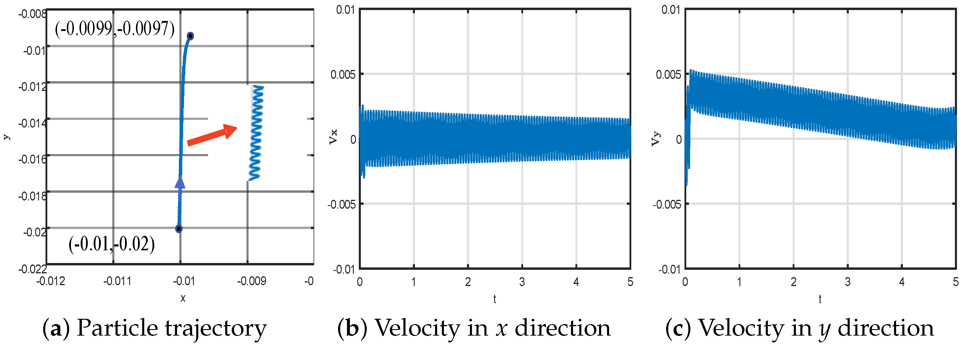
2.2. Simulations Analysis

For the square silicon thin plate with $l=5$ cm, $h=0.0625$ cm, the first three vibration modes are summarized in

Table 1. Vibration modes.

m	n	${\mathit{\omega }}_{\mathit{mn}}$
1	1	126.5475
1	2	315.5072
1	3	631.0144

. Necessarily, combining Equations (2) and (3), the acceleration components of the thin plate material pointing along the unit vectors ${\mathrm{e}}_x,{\mathrm{e}}_y,{\mathrm{e}}_z$ can be obtained as

$$\left\{\begin{array}{c}{a}_{Tz}(x,y,t)=\ddot{w}(x,y,t)=-A{\omega }_{mn}^{2}sin\left({\omega }_{mn}t\right)sin\frac{m\pi x}{l}sin\frac{n\pi y}{l}\hfill \\ a_{Tx}(x,y,t)={\ddot{w}}_{,x}(x,y,t)=A{\omega }_{mn}^2\frac{m\pi h}{2l}sin\left({\omega }_{mn}t\right)cos\frac{m\pi x}{l}sin\frac{n\pi y}{l}\hfill \\ a_{Ty}(x,y,t)={\ddot{w}}_{,y}(x,y,t)=A{\omega }_{mn}^2\frac{n\pi h}{2l}sin\left({\omega }_{mn}t\right)sin\frac{m\pi x}{l}cos\frac{n\pi y}{l}\hfill \end{array}\right.$$

(8)

Referring to the analysis in Section 2.1, the kinematic modes of a particle on the excited plate can be numerically solved. Here, the first three vibration modes (shown in Table 1) were applied to perform the modal distribution using the the mathematical conditions in the last sub-section. All of the parameters were set in accordance with the actual platform, plate density $\rho =2329{\mathrm{g}/\mathrm{m}}^3$, Young’s modulus $E=170\times {10}^9$, Poisson’s ratio $\upsilon =0.28$, and friction coefficient $\mu =0.02$.

The distribution maps of the motion modes corresponding to the first third-order vibration modes are represented by the three subgraphs in Figure 3 drawn by using Matlab(R2020b) with $t=0.5$ s. The particle sliding motion region in the figure is represented by the shadow portion of the dotted line, whereas the particle fixing motion area is represented by the blue area and the particle bouncing motion area by the white area, as shown in the text description of Figure 3a. From Figure 3a–c, the three kinematic modes are distributed in the coordinate plane in a centrally symmetric manner. Along the y-axis direction, the sliding region and the bouncing region alternate. The surface area of the particle stationary zone rapidly reduces as the vibration mode rises ($m=1,n=1$,$m=1,n=2$ to $m=1,n=3$), and the frequency of the conversion between the sliding motion and bouncing motion areas increases as the vibration mode increases.

The vibration modes are displayed at $(m,n)=(1,1)$ and $(m,n)=(1,3)$, respectively, to examine how amplitude A affects the motion modes distribution. These motion mode distribution diagrams are then compared: Figure 3a with Figure 4a, and Figure 3c with Figure 4b. The distribution and switching rules of the particle motion mode are unaffected by amplitude changes; however, the area of the particle fixed area is drastically reduced under the corresponding vibration mode.

3. Dynamics of the Particle

The previous analysis shows that, once the geometric conditions of the thin plate are determined, there may be three different motion modes of particles with zero initial velocity on the thin plate under the excitation of a certain characteristic frequency, and the distribution of particles in the bouncing, sliding, and fixed areas is uniquely determined under the condition that the excitation signal remains unchanged. The dynamics of particles in the sliding area are examined in the following analysis.

On the particle sliding area, the velocity ${\mathrm{v}}_T$ of any material point in the sheet surface is described as:

$${\mathrm{v}}_T(x,y,t)={\mathrm{v}}_{Tx}{\mathrm{e}}_x+{\mathrm{v}}_{Ty}{\mathrm{e}}_y$$

(9)

The velocity of particles ${\mathrm{v}}_P$ on the plane is described as:

$${\mathrm{v}}_P(x,y,t)={\dot{x}}_P{\mathrm{e}}_x+{\dot{y}}_P{\mathrm{e}}_y$$

(10)

The sliding friction force of particles in two directions of the plate plane can be expressed as:

$$\left\{\begin{array}{c}{f}_x=-\mu N\frac{({\mathrm{v}}_P-{\mathrm{v}}_T)}{\left|({\mathrm{v}}_P-{\mathrm{v}}_T)\right|}{\mathrm{e}}_x\hfill \\ f_y=-\mu N\frac{({\mathrm{v}}_P-{\mathrm{v}}_T)}{\left|({\mathrm{v}}_P-{\mathrm{v}}_T)\right|}{\mathrm{e}}_y\hfill \end{array}\right.$$

(11)

which is defined according to the component of the difference between particle velocity ${\mathrm{v}}_P$ and plate velocity ${\mathrm{v}}_T$ on the $x,y$ directions, respectively.

The particle dynamics in the vertical direction and x-y planes are given in Equation (4). The particle dynamics model under sliding mode can be obtained simultaneously using Equations (4) and (11) as follows:

$$\left\{\begin{array}{c}{\ddot{x}}_P=-\mu (a_{Tz}(x,y,t)+g)\frac{({\dot{x}}_P-v_{Tx}(x,y,t))}{\sqrt{{({\dot{x}}_P-v_{Tx}(x,y,t))}^2+{({\dot{y}}_P-v_{Ty}(x,y,t))}^2}}\hfill \\ {\ddot{y}}_P=-\mu (a_{Tz}(x,y,t)+g)\frac{({\dot{y}}_P-v_{Ty}(x,y,t))}{\sqrt{{({\dot{x}}_P-v_{Tx}(x,y,t))}^2+{({\dot{y}}_P-v_{Ty}(x,y,t))}^2}}\hfill \end{array}\right.$$

(12)

In this way, the interaction between the particle and plate N can be eliminated.

In Equation (12), the velocities of the thin plate material point in the x and y directions can be obtained by integrating the corresponding acceleration components, which have been shown in Equation (8).

$$\left\{\begin{array}{c}{v}_{Tx}=\int a_{Tx}(x,y,t)dt=-A{\omega }_{mn}^{}\frac{m\pi h}{2l}cos\left({\omega }_{mn}t\right)cos\frac{m\pi x}{l}sin\frac{n\pi y}{l}\hfill \\ v_{Ty}=\int a_{Ty}(x,y,t)dt=-A{\omega }_{mn}^{}\frac{n\pi h}{2l}cos\left({\omega }_{mn}t\right)sin\frac{m\pi x}{l}cos\frac{n\pi y}{l}\hfill \end{array}\right.$$

(13)

Substituting the velocity expression of the material point in Equation (13) into Equation (12), we can obtain the specific expression of the particle motion model in the sliding area of the acoustic driven thin plate as follows:

$$\left\{\begin{array}{c}{\ddot{x}}_P=-\mu (-A{\omega }_{mn}^{2}sin\left({\omega }_{mn}t\right)sin\frac{m\pi x}{l}sin\frac{n\pi y}{l}+g)\ast \hfill \\ \frac{({\dot{x}}_P+A{\omega }_{mn}^{}\frac{m\pi h}{2l}cos\left({\omega }_{mn}t\right)cos\frac{m\pi x}{l}sin\frac{n\pi y}{l})}{\sqrt{{({\dot{x}}_P+A{\omega }_{mn}^{}\frac{m\pi h}{2l}cos\left({\omega }_{mn}t\right)cos\frac{m\pi x}{l}sin\frac{n\pi y}{l})}^2+{({\dot{y}}_P+A{\omega }_{mn}^{}\frac{n\pi h}{2l}cos\left({\omega }_{mn}t\right)sin\frac{m\pi x}{l}cos\frac{n\pi y}{l})}^2}}\hfill \\ \\ {\ddot{y}}_P=-\mu (-A{\omega }_{mn}^{2}sin\left({\omega }_{mn}t\right)sin\frac{m\pi x}{l}sin\frac{n\pi y}{l}+g)\ast \hfill \\ \frac{({\dot{y}}_P+A{\omega }_{mn}^{}\frac{n\pi h}{2l}cos\left({\omega }_{mn}t\right)sin\frac{m\pi x}{l}cos\frac{n\pi y}{l})}{\sqrt{{({\dot{x}}_P+A{\omega }_{mn}^{}\frac{m\pi h}{2l}cos\left({\omega }_{mn}t\right)cos\frac{m\pi x}{l}sin\frac{n\pi y}{l})}^2+{({\dot{y}}_P+A{\omega }_{mn}^{}\frac{n\pi h}{2l}cos\left({\omega }_{mn}t\right)sin\frac{m\pi x}{l}cos\frac{n\pi y}{l})}^2}}\hfill \end{array}\right.$$

(14)

In addition, when particles are in the fixing area on the plate, the movement of particles is the same as that of the thin plate material point; that is to say, ${\mathrm{v}}_T(x,y,t)={\mathrm{v}}_P(x,y,t)$. Furthermore, the particle dynamics of sliding motion governed by Equation (14) is analyzed. Here, the first vibration mode ($m=n=1$) was applied, and the corresponding excitation frequency was $f=126.5475$ Hz. The simulation step size and termination time were, respectively, set as $\Delta t=1\times {10}^{-5}$ s, $t=5$ s. In particular, the acoustic amplitude $A=0.1$, and the initial velocity of particles in two directions was set as ${\dot{x}}_p=0.0001,$${\dot{y}}_p=0.0001.$

Notably, all of the starting points of the simulations were set at the sliding regions so that the derived dynamics model was valid. Figure 5a and Figure 6a reflect the particle trajectory of the two simulations, respectively, within 5 s. In Figure 5a, the start point is (0.01, 0.01) and the terminal point is (0.01, 0.0197). The trajectory is located at the region of the first quadrant of the thin plate. It can be seen that, although the particle produces a displacement of one centimeter in the sliding area, the track changes constantly as the trajectory enlarges, as shown in Figure 5a. Complementarily, Figure 5b,c express that the velocities along x and y directions change strongly, which shows that the particle motion on the thin plate has a high speed variation and great uncertainty. Another start point is chosen at the third quadrant of the thin plate shown in Figure 6a–c, whose trajectory starts at (−0.01, −0.02) and ends at (−0.0099, −0.0097), and similar rules can be drawn. Moreover, the particle motion trajectory in the sliding area is always in the positive direction of the y-axis. As a result, the motion of the particle in the sliding region of the driven plate has a strong uncontrollability and variability, and, regarding any sliding area on the thin plate, such motion trajectory and features exist.

4. Particle Trajectory Control Based on Ladrc

Micro-nano particle motion on the driven thin plate is a rather complicated process, and it is also a very challenging problem for particle kinematics modeling. From the modeling and analysis in Section 3, during particle movement, the velocity and displacement direction of the particle are both constantly changing. Hence, the particle is in irregular motion. In order to further follow the particle trajectory and realize the basic linear trajectory control, the LADRC algorithm is applied in this section [38,39].

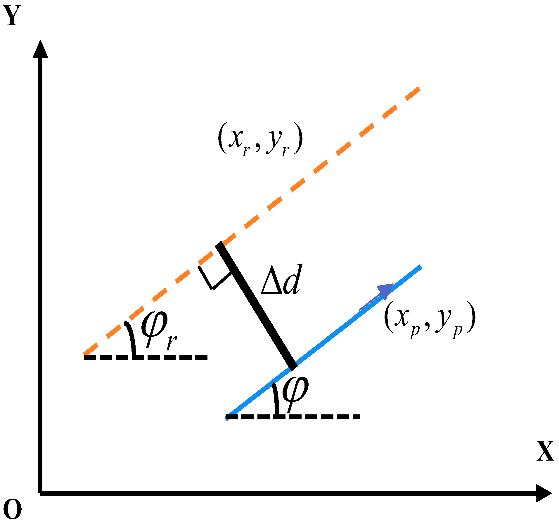
4.1. Control Algorithm and Mechanism

From the particle dynamic model derived above, the acoustic signal is an important quantity used to control the particle trajectory. The excitation frequency and amplitude of the driven signal are the important control variables. Nevertheless, if the signal of the driving frequency is changed randomly, the distribution of particle motion modes will change significantly, so the control process should be carried out under a certain frequency. In this sub-section, we chose the first order vibration mode as it has the larger continuous sliding region ($2.5$ cm × 1 cm) in each quadrant of the plate coordinate plane. Therefore, the amplitude A was considered as the controlling variable of the particle trajectory control task.

As a description, the mechanism of the control task for the linear trajectory is shown in Figure 7. According to the mechanism, the line reference track is set as the orange dotted line shown in Figure 7, and any point on it is marked as $(x_r,y_r)$. The particle path based on the sliding mathematical model is indicated by the blue solid line, and any point of it is represented by $(x_p,y_p)$. Assume that the blue arrow indicates the direction of particle movement. The distance between the reference track and particle path is $▵d$, characterizing the tracking error. Consequently,

$$\Delta d^2={(x_P-x_r)}^2+{(y_P-y_r)}^2.$$

(15)

On the other hand, the included angle between the reference track and x-axis is ${\phi }_r$. The included angle between the particle path and x-axis is ${\phi }_P$. ${\phi }_r$ and ${\phi }_P$ are, respectively, defined as

$$\left\{\begin{array}{c}{\phi }_r=arctan\left(\frac{y_r}{x_r}\right)\hfill \\ {\phi }_P=arctan\left(\frac{y_p}{x_p}\right)\hfill \end{array}\right..$$

(16)

During trajectory control, if the conditions $\Delta d\approx 0$ and ${\phi }_p-{\phi }_p\approx 0$ are all well-controlled, the particle path will follow the reference track. For the control problem discussed in this paper, the amplitude A was used to control the movement of the particle in x and y directions. Further, the non-linear combination was designed for performing this under-actuated control problem as

$$E=\Delta d^2+K\ast ({\phi }_P-{\phi }_r)$$

(17)

in which, K is an adjustable positive factor. According to the geometric mechanism and the proposed non-linear combination, when a good control effect is achieved, $E=0$, so $E=0$ is the control target. As the controller of LADRC does not need precise information, the order of the controlled system is necessary. Then, we will solve this relationship. Combining Equations (14)–(17),

$$\ddot{E}={(\Delta d^2)}^{{}^{″}}+K\ast {(arctan\left(\frac{y_p}{x_p}\right)-arctan\left(\frac{y_r}{x_r}\right))}^{{}^{″}}$$

(18)

Finally, a second-order system can be obtained as

$$\ddot{E}=f({\dot{x}}_P,{\dot{y}}_P,x_P,y_P,\tau \left(A\right))+b_{1}A$$

(19)

in which, $f({\dot{x}}_P,{\dot{y}}_P,x_P,y_P,\tau \left(A\right))$ is regarded as the disturbance of the system, and $b_1$ is a constant. Based on the LADRC, the control core is used to estimate the disturbance and ignore disturbance. Set $x_1=E,x_2=\dot{E},x_3=f$, and define the following system:

$$\left\{\begin{array}{c}{\dot{x}}_1=x_2\hfill \\ {\dot{x}}_2=x_3+b_{1}A\hfill \\ {\dot{x}}_3=\dot{f}\hfill \end{array}\right.$$

(20)

Then, the corresponding linear expanded state observer (LESO) was designed as below:

$$\left\{\begin{array}{c}{\dot{z}}_1=z_2-3{\omega }_o(z_1-x_1)\hfill \\ {\dot{z}}_2=z_3-3{\omega }_o^2(z_1-x_1)+b_{1}A\hfill \\ {\dot{z}}_3=-{\omega }_o^3(z_1-x_1)\hfill \end{array}\right.$$

(21)

in which, $z_1,z_2,z_3$ are, respectively, the estimated values of $x_1,x_2,x_3$. By adjusting the ${\omega }_o$, the observer bandwidth, then an ideal estimated effect $z_3$≈$f({\dot{x}}_P,{\dot{y}}_P,x_P,y_P,\tau \left(A\right))$.

Consequently, the following control law is proposed:

$$A=\frac{K_p(-z_1)+K_d(-z_2)-z_3}{b_1}$$

(22)

where $K_p$ and $K_d$ are the feedback control gains.

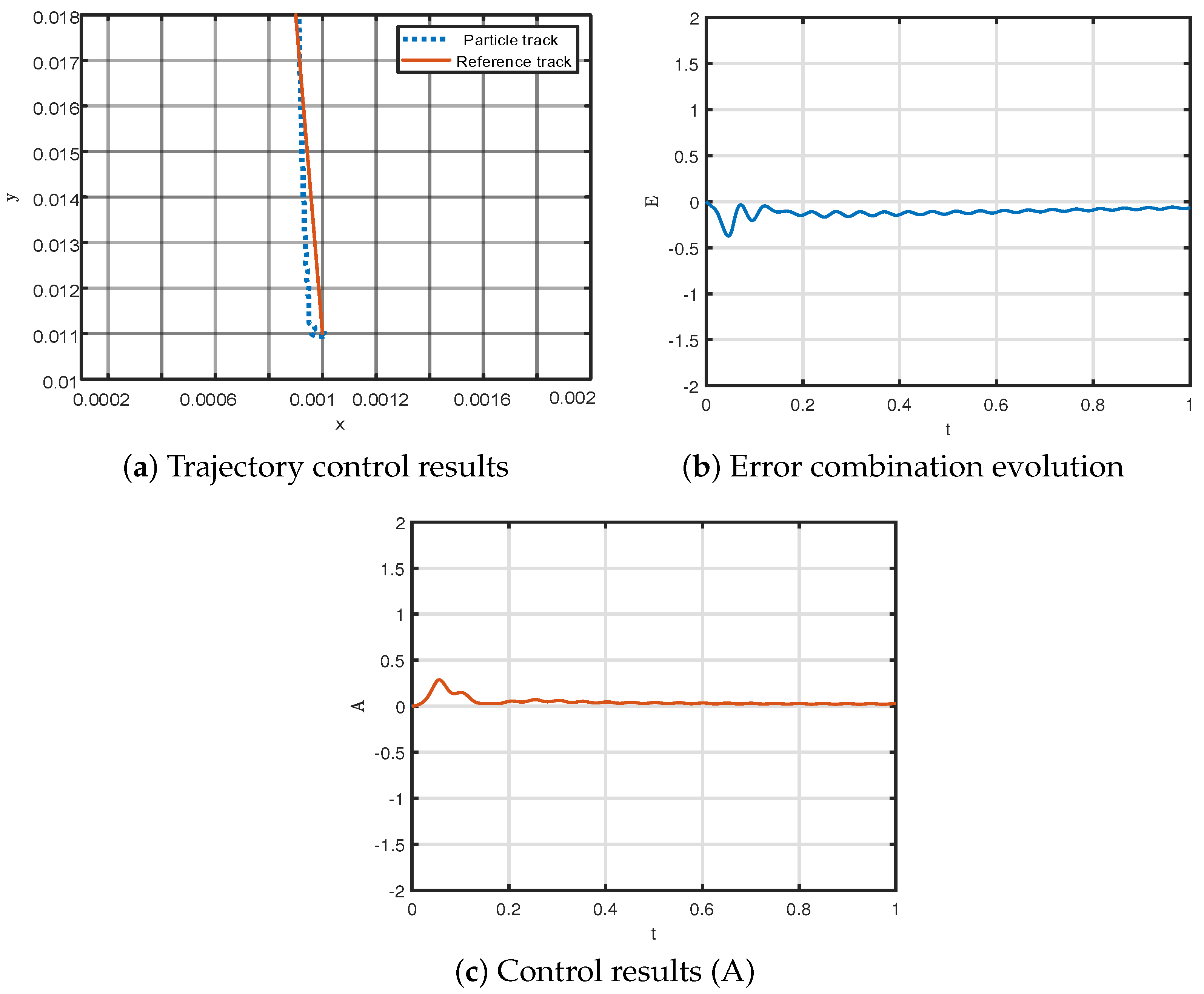
4.2. Control Results Simulation

Section 4.1 explains the control principle and concept. The path following task for the sliding region is implemented here. The start point must be located on the sliding region of the thin plate during this process, and a reference trajectory must be established first. The ultimate position of the particle should also be within the sliding area to ensure the validity of the particle model. From Figure 3, the particle sliding region is regularly distributed on the surface of thin plate. Here, two cases of different starting points and reference paths are displayed, whose routes are located in various sliding areas of the thin plate.

For the first case, the start point was set as (0.001, 0.011), located in the first quadrant of the sheet coordinates, $x_r=0.001-0.0001t,y_r=0.011+0.007t$, the reference trajectory. The relative parameters were $b_1=30,{\omega }_0=3.5,K_p=45,K_d=25,K=80$. The start point of the second case was placed as (−0.001, 0.001), the second quadrant of the sheet coordinates, $x_r=-0.001-0.0001t,y_r=0.001+0.009t$, the reference trajectory, and the relative parameters were $b_1=11,{\omega }_0=3.5,K_p=8,K_d=25,K=3.1$. The orange track represents the reference trajectory in the simulation results given in Figure 8a and Figure 9a; the blue dotted line track represents the tracking outcomes. It is worth mentioning that the particle trajectory can not only complete the tracking task, but also the displacement direction will not change frequently. From the comparison between the particle trajectory and reference trajectory, the particle traces the reference track under the control mechanism described in Section 4.1, and is guided by the control law to travel within the permissible error range. Additionally, the control target $E=0$ is also checked, as shown in the simulation results in Figure 8b and Figure 9b, and the control results (actual A) for two cases are, respectively, reported in Figure 8c and Figure 9c. It can be seen that the designed non-linear combination E is approximately equal to 0, which further reflects the control effects. On the whole, the particle trajectory can be controlled by LADRC with necessary mathematical support.

5. Conclusions

Acoustic manipulation is regarded as a novel method for controlling micro-nano targets, with little theoretical research and analysis available. This paper is concerned with particle motion on a thin plate and its control based on an acoustic signal driving it. First, a particle-based plate space coordinate system was created. The modes of particle motions on driven plates were identified by combining particle Newton kinematics analysis with the theory of thin plate vibration. The motions of bouncing, sliding, and fixing on the plate were uniquely determined under a specific vibration mode when the corresponding mathematical conditions were met. Furthermore, the rules of modes distributions according to the frequencies and amplitudes were summarized. Next, on the region of the particle sliding mode, the particle dynamics was deduced, and its trajectory characteristics were also revealed through numerical simulations. Finally, the particle path following control was performed using the LADRC method, resulting in a preliminary control effect for linear trajectory. More accurate and complex path control will be a key issue to discuss in the future to direct practical applications.

References

1. Utadiya, S.; Joshi, S.; Patel, N.; Patel, C.; Joglekar, M.; Cahhniwal, V.; O’Connor, T.; Javidi, B.; An, A. Integrated self-referencing single shot digital holographic microscope and optical tweezer. Light. Adv. Manuf. 2022, 3, 37. [Google Scholar] [CrossRef]
2. Kotnala, A.; Gordon, R. Double nanohole optical tweezers visualize protein p53 suppressing unzipping of single DNA-hairpins. Biomed. Opt. Express 2014, 5, 1886–1894. [Google Scholar] [CrossRef] [Green Version]
3. Tao, T.; Li, J.; Long, Q.; Wu, X. 3D trapping and manipulation of micro-particles using holographic optical tweezers with optimized computer-generated holograms. Chin. Opt. Lett. 2011, 9, 120010. [Google Scholar] [CrossRef]
4. Zhu, X.; Li, N.; Yang, J.; Chen, X. Revolution of trapped particle in counter-propagating dual-beams optical tweezers under low pressure. Opt. Express 2021, 29, 11169–11180. [Google Scholar] [CrossRef] [PubMed]
5. Thomas, R.G.; Unnithan, A.R.; Moon, M.J.; Surendran, S.P.; Batgerel, T.; Park, C.H.; Kim, C.S.; Jeong, Y.Y. Electromagnetic manipulation enabled calcium alginate Janus microsphere for targeted delivery of mesenchymal stem cells. Int. J. Biol. Macromol. Struct. Funct. Interact. 2018, 110, 465–471. [Google Scholar] [CrossRef]
6. Yu, S.; Cheng, J.; Li, Z.; Liu, W.; Cheng, H.; Tian, J.; Chen, S. Electromagnetic wave manipulation based on few-layer metasurfaces and polyatomic metasurfaces. Chem. Phys. Mater. 2022, 1, 6–16. [Google Scholar] [CrossRef]
7. Wang, Y.; Luo, L.; Ke, M.; Liu, Z. Acoustic Subwavelength Manipulation of Particles with a Quasiperiodic Plate. Phys. Rev. Appl. 2022, 17, 014026. [Google Scholar] [CrossRef]
8. Zhou, Q.; Sariola, V.; Latifi, K.; Liimatainen, V. Controlling the motion of multiple objects on a Chladni plate. Nat. Commun. 2016, 7, 12764. [Google Scholar] [CrossRef] [Green Version]
9. Wijaya, H.; Latifi, K.; Zhou, Q. Two-Dimensional Manipulation in Mid-Air Using a Single Transducer Acoustic Levitator. Micromachines 2019, 10, 257. [Google Scholar] [CrossRef] [Green Version]
10. Ahmed, D.; Ozcelik, A.; Bojanala, N. Rotational manipulation of single cells and organisms using acoustic waves. Nat. Commun. 2016, 7, 5120–5125. [Google Scholar] [CrossRef]
11. Lee, T.; Kwon, H.B.; Song, W.; Lee, S.; Kim, Y.J. Microfluidic ultrafine particle dosimeter using an electrical detection method with a machine-learning-aided algorithm for real-time monitoring of particle density and size distribution. Lab Chip 2021, 21, 1503–1516. [Google Scholar] [CrossRef] [PubMed]
12. Jia, W.N.; Neild, A. Multiple outcome particle manipulation using cascaded surface acoustic waves (CSAW). Microfluid. Nanofluid 2021, 25, 16. [Google Scholar]
13. Yiannacou, K.; Sariola, V. Controlled Manipulation and Active Sorting of Particles Inside Microfluidic Chips Using Bulk Acoustic Waves and Machine Learning. Langmuir 2021, 37, 4192–4199. [Google Scholar] [CrossRef]
14. Xu, D.; Cai, F.Y.; Chen, M. Acoustic manipulation of particles in a cylindrical cavity: Theoretical and experimental study on the effects of boundary conditions. Ultrasonics 2019, 93, 4192–4199. [Google Scholar] [CrossRef] [PubMed]
15. Hu, J.H. An introduction to acoustic micro/nano manipulations. Appl. Phys. 2016, 6, 114–118. [Google Scholar] [CrossRef]
16. Devendran, C.; Collins, D.J.; Neild, A. The role of channel height and actuation method on particle manipulation in surface acoustic wave (SAW)-driven microfluidic devices. Microfluid. Nanofluid. 2022, 26, 9. [Google Scholar] [CrossRef]
17. Luo, Y.; Feng, R.; Li, X.; Liu, D. A simple approach to determine the mode shapes of Chladni plates based on the optical lever method. Eur. J. Phys. 2019, 40, 065001. [Google Scholar] [CrossRef]
18. Tuan, P.H.; Wen, C.P.; Chiang, P.Y.; Yu, Y.T. Exploring the resonant vibration of thin plates: Reconstruction of Chladni patterns and determination of resonant wave numbers. J. Acoust. Soc. Am. 2015, 137, 2113–2123. [Google Scholar] [CrossRef] [Green Version]
19. Grabec, I. Vibration driven random walk in a Chladni experiment. Phys. Lett. A 2017, 381, 59–64. [Google Scholar] [CrossRef]
20. Greshilov, A.G.; Sukhinin, S.V. Chladni figures of acircular plate floating in bounded and unbounded water bodies with securing support at the center. Sib. Zhurnal Ind. Mat. 2017, 20, 31–40. [Google Scholar]
21. Ding, X.Y.; Lin, S.C.S.; Kiraly, B. On-chip manipulation of single microparticles, cells, and organisms using surface acoustic waves. Proc. Natl. Acad. Sci. USA 2012, 109, 11105–11109. [Google Scholar] [CrossRef] [PubMed] [Green Version]
22. Fornell, A. Droplet microfluidics. In Acoustic Manipulation of Cells and Microbeads in Droplet Microfluidics; Department of Biomedical Engineering, Lund University: Lund, Sweden; Publishing House: Lund, Sweden, 2018. [Google Scholar]
23. Teruyuki, K.; Takuya, Y.; Masahiro, T.; Shin-ichi, H. Two-dimensional acoustic manipulation in air using interference of standing wave field by three sound waves. Jpn. J. Appl. Phys. 2022, 62, SG1063. [Google Scholar]
24. Ali, N.; Mohsen, E.H.; Saeed, E.A.; Javad, V.A. Vibration of a thin rectangular plate subjected to series of moving inertial loads. Mech. Res. Commun. 2014, 55, 105–113. [Google Scholar]
25. Aman, K.; Anirvan, D. Wave-induced dynamics of a particle on a thin circular plate. Nonlinear Dyn. 2021, 103, 293–308. [Google Scholar]
26. Zaslavskii, O.B. Acceleration of particles by rotating black holes: Near-horizon geometry and kinematics. Gravit. Cosmol. 2011, 2, 139–142. [Google Scholar] [CrossRef]
27. Fleishman, D.; Asscher, Y.; Urbakh, M. Directed transport induced by asymmetric surface vibrations: Making use of friction. J. Phys. Condens. Matter 2007, 19, 096004. [Google Scholar] [CrossRef] [Green Version]
28. Zewei, H.; Zhitao, Z.; Zengyao, L.; Yongmao, P. Particles separation using the inverse Chladni pattern enhanced local Brazil nut effect. Extrem. Mech. Lett. 2021, 49, 101466. [Google Scholar]
29. Ikpe, A.E.; Ndon, A.E.; Etuk, E.M. Response variation of chladni patterns on vibrating elastic plate under electro-mechanical oscillation. Niger. J. Technol. 2019, 30, 540–548. [Google Scholar] [CrossRef] [Green Version]
30. Ali, N.; Fayaz, R.R. Parametric study of the dynamic response of thin rectangular plates traversed by a moving mass. Acta Mech. 2012, 223, 15–27. [Google Scholar]
31. Qinghua, S.; Jiahao, S.; Zhanqiang, L.; Yi, W. Dynamic analysis of rectangular thin plates of arbitrary boundary conditions under moving loads. Int. J. Mech. Sci. 2016, 117, 16–29. [Google Scholar]
32. Zheng, Y.; Tao, J.; Sun, Q.; Sun, H.; Chen, Z.; Sun, M.; Xie, G. Soft Actor-Critic based active disturbance rejection path following control for unmanned surface vessel under wind and wave disturbances. Ocean Eng. 2022, 247, 110631. [Google Scholar] [CrossRef]
33. Wang, Y.; Chen, Z.; Sun, M.; Sun, Q.; Piao, M. On Sign Projected Gradient Flow Optimized Extended State Observer Design for a Class of Systems with Uncertain Control Gain. IEEE T Ind. Electron. 2021, 70, 773–782. [Google Scholar] [CrossRef]
34. Bie, G.; Chen, X. UAV trajectory tracking based on ADRC control algorithm. In ITM Web of Conferences; EDP Sciences: Les Ulis, France, 2022; Volume 47, p. 02017. [Google Scholar]
35. Karimi, A.H.; Alahdadi, S.; Ghayour, M. Dynamic analysis of a rectangular plate subjected to a mass moving with variable velocity on a predefined path or an arbitrary one. Thin-Walled Struct. 2021, 160, 107340. [Google Scholar] [CrossRef]
36. Park, I.; Lee, U.; Park, D. Transverse Vibration of the Thin Plates: Frequency-Domain Spectral Element Modeling and Analysis. Math. Probl. Eng. Theory Methods Appl. 2015, 24, 1–15. [Google Scholar] [CrossRef] [Green Version]
37. Henk, J.G.; Martin, A.; Devaraj, M.; Ko, W. Inversion of Chladni patterns by tuning the vibrational acceleration. Phys. Rev. E 2010, 82, 012301. [Google Scholar]
38. Bettayeb, M.; Mansouri, R.; Al-Saggaf, U.M.; Al-Saggaf, A.U.; Moinuddin, M. New LADRC scheme for fractional-order systems. Alex. Eng. J. 2022, 61, 11313–11323. [Google Scholar] [CrossRef]
39. Chang-Mei, H.U.; Ren, J. Study and Application of LADRC for Drum Water-Level Cascade Three-Element Control. Electr. Power 2014, 47, 1–4. [Google Scholar]
Figure 1. Acoustic manipulation platform.
Mathematics 10 04156 g001
Figure 2. Thin plate space coordinate system.
Mathematics 10 04156 g002
Figure 3. Particle motion modes distribution results of the first three vibration modes with A = 0.1 .
Mathematics 10 04156 g003
Figure 4. Particle motion modes distribution results with A = 10 .
Mathematics 10 04156 g004
Figure 5. Particle trajectory simulation in sliding region of the first quadrant.
Mathematics 10 04156 g005
Figure 6. Particle trajectory simulation in sliding region of the third quadrant.
Mathematics 10 04156 g006
Figure 7. Mechanism of linear trajectory control.
Mathematics 10 04156 g007
Figure 8. Control effects with initial conditions ( x P = 0.001, y P = 0.011).
Mathematics 10 04156 g008
Figure 9. Control effects with initial conditions ( x P = −0.001, y P = 0.001).
Mathematics 10 04156 g009