1. Introduction
Community detection is a fundamental task in complex network analysis, which aims to partition a network into multiple substructures (communities). Usually, a community is defined as a set of nodes with a different affiliation from the rest of the network [
1]. Community detection has been extensively studied and applied in many real-world network problems, such as recommendation [
2], anomaly detection [
3], and terrorist organization identification [
4]. Classical community detection methods usually utilize probabilistic models and statistical inference methods. These methods employ different varieties of prior knowledge to infer community structure. For example, classical community detection methods, spectral clustering [
5], GN algorithm [
6], etc. However, traditional community detection algorithms usually focus only on the network structure and often ignore the attributes of nodes, resulting in a lack of semantic community division. In the real world, the attributes of nodes are becoming more affluent and more prosperous, and a more reasonable solution is to consider both the relationships between nodes and semantic information. For community detection in attribute networks, a balance should be achieved between the following two properties: (1) structural closeness, i.e., nodes within a community are structurally close to each other, while nodes in different communities are not, and (2) attribute homogeneity, i.e., nodes in a community have similar attributes, while nodes in different ones are different [
7].
Community detection is a typical application of graph clustering. For attributed graph clustering, capturing the network topology and utilizing the content information of nodes is a crucial problem. The method based on graph embedding obtains the node low-dimensional vector representation by learning the network topology and node content [
8]. On this basis, the current research focus is the application of clustering methods such as K-means to solve the problem of community detection. The autoencoder is the mainstream solution for graph embedding-based methods [
9], because the autoencoder-based representation can be applied to unsupervised scenarios. Inspired by the above methods, we use an autoencoder and a graph neural network as the basic framework for attribute graph clustering.
In this paper, we propose a community detection fusing graph attention network (CDFG) model. The main contributions are: (1) we fuse the autoencoder and the graph attention network with high-order neighborhood information for the first time. (2) We design the feature fusion module. Specifically, the graph attention layer in the graph attention network [
10] aggregates node feature information in the neighborhood by trainable weights and considers the different extent of influence of neighborhood nodes on the target node. Then we obtain the high-order neighborhood information of the target node by calculating the topological correlation matrix. The correlation between nodes is fully utilized. The feature fusion module calculates the self-correlation matrix by taking the hidden layer representation obtained from the graph attention network and then multiplies the obtained autocorrelation matrix with the matrix obtained from the graph attention module to obtain the final node representation using the principle of jump connection. The results of conducted experiments on six real datasets and evaluating the model using four evaluation metrics show that the model performs better than other methods.
2. Related Work
2.1. Traditional Methods
Traditional methods are based on network topology for community detection, which can be divided into graph partitioning, statistical inference, hierarchical clustering, dynamic methods, spectral clustering, density-based methods, and optimization methods according to the principles applied [
11]. These methods only capture the shallow structure of the network and have a high computational complexity for large-scale network data. With the increasing richness of information in the real world, traditional community detection methods can no longer meet demands.
2.2. Graph Embedding Methods
Graph embedding methods can map high-dimensional sparse vectors into low-dimensional dense vectors with the advantage of using high-dimensional nonlinear features (e.g., network topology information) and high-dimensional relational features (e.g., node attribute information) represented by nodes, neighbors, edges, subgraphs (e.g., communities), and encoded features [
12]. In this kind of method, the nodes in a complex network are represented by low-dimensional real-value vectors, and the traditional clustering method can be used to solve the community detection problem. At present, deep clustering approaches focuses on the graph convolutional network-based approaches and autoencoder-based approaches.
Clustering methods based on graph convolutional networks (GCN) [
13] to learn graph structure and node attributes have been widely studied [
14,
15,
16,
17,
18,
19,
20,
21,
22,
23]. For attribute graphs, neighboring nodes and nodes with similar characteristics may gather in the same community. Graph autoencoders (GAE) and variational graph autoencoders (VGAE) [
14] integrate graph structures into node attributes by iteratively aggregating the neighborhood representation around each central node. Deep attentional embedded graph clustering (DAEGC) [
15] uses a graph structure and node attributes at the same time. It captures the importance of the neighborhood nodes through a graph attention network as an encoder and uses KL-divergence loss to supervise the training process of graph clustering. On the basis of DAEGC, the deep-neighbor-aware embedding for node clustering in attributed graphs (DNENC) [
16] uses GCN as the encoder, which complements the contrast experiments. The experimental results show the effectiveness of the proposed framework. According to the setting of DAEGC, the adversarially regularized graph autoencoder (ARGA) [
17] further developed an adversarial regulator to guide the learning of potential representations. Structural deep clustering network (SDCN) [
18] integrates an information transfer operator, a dual self-supervised learning mechanism, an autoencoder, and a graph convolution network into a unified framework for better representation learning better. Experiments show that the autoencoder can alleviate the over-fitting phenomenon. The hierarchical attention network (HiAN) [
23] designs the hierarchical attentive aggregator to fuse rich interpretable interactive information. These GCN-based methods still have the problem of smoothing. Meanwhile, GCN only aggregates neighborhood information equally when learning structural representation.
Many deep clustering methods based on the autoencoder also have been proposed [
24,
25,
26,
27]. The autoencoder (AE) [
28] is the most commonly used solution for unsupervised community detection. Deep embedded clustering (DEC) [
24] first trains the encoder and then uses a pretrained network to iteratively optimize the KL divergence-based clustering loss with the help of self-learning-assisted target distributions so that the representation learned by the autoencoder is closer to the center of the clusters and improves the cohesiveness of the clusters. To improve the accuracy of the target distribution, the improved deep embedded clustering (IDEC) [
25] jointly optimizes the clustering assignment and learns features suitable for clustering while maintaining local structure. These methods help the autoencoder learn data representations with higher relevance to clustering by computing clustering loss, exploiting the features of the data itself but not incorporating structural information.
3. The Proposed Model
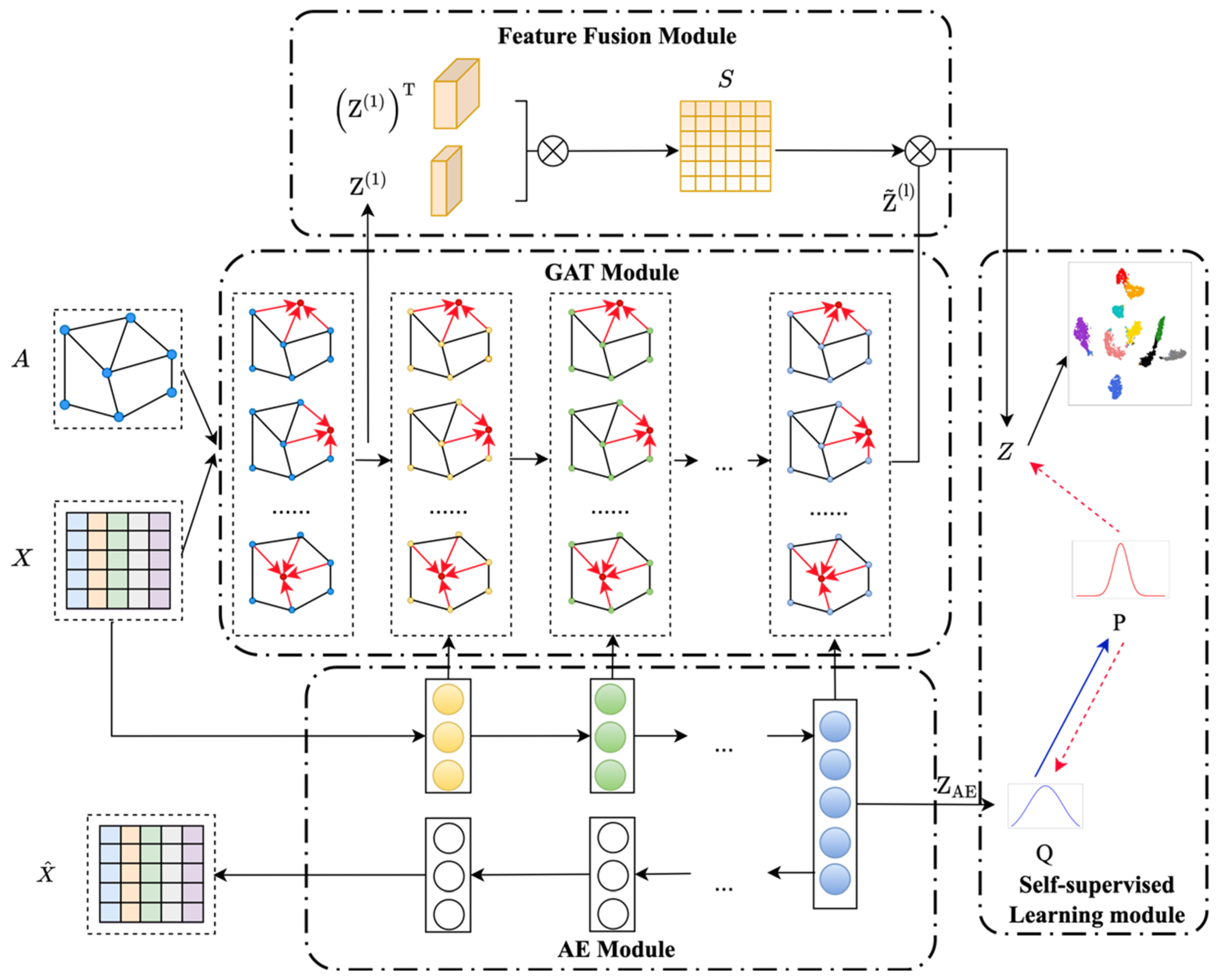
In this section, we present the community detection fusing graph attention network (CDFG) shown in
Figure 1. We first introduce the notation and the problem definition. In the following subsections, we describe the CDFG model in detail in four modules, i.e., the autoencoder module (AE), the graph attention network module (GAT), the feature fusion module, and the self-supervision learning module.
A complex network whose nodes have attributes is an attribute network. Given an attribute network , where is the set of nodes, is the set of edges. is the number of nodes. is the feature matrix, where denotes the attribute vector of node . Here, is the attribute dimension. The topology of the graph can be represented by the adjacency matrix and if , , otherwise .
Problem Definition. Given an attribute network , it is divided into several disjoint groups, i.e., . Each community is a partition of the network , and represents the number of communities divided from the original network with common properties of clustering. Nodes in the same community should satisfy to be structurally tightly connected and have more similar attributes, while nodes in different communities are sparsely connected and have different attributes. means that there is no intersection between communities, indicating non-overlapping community detection.
3.1. AE Module
A basic autoencoder [
28] is used for unsupervised representation learning of the data from the perspective of generality to extract valid information from the attribute features of the data itself. The autoencoder consists of an encoder and a decoder. The encoder maps the input data to a particular feature space to obtain the hidden layer representation, and the decoder maps the hidden layer representation to the input space. It makes the hidden layer representation retain the features of the input data through the reconstruction of the input data. We suppose there are
layers in the autoencoder and
denotes the
-th layer of the autoencoder, then the learning representation
of the
-th layer of the encoder part is formulated as:
where
is the activation function,
is the
-th layer weight matrix, and
is the bias of the
-th layer in the encoder.
The decoder and the encoder are symmetric, and the corresponding learning representation
is calculated as:
where
is the
-th layer weight matrix and
is the bias of the
-th layer in the decoder.
The objective function can be obtained by minimizing the loss between the original data and the reconstruction:
where
is the reconstruction of the original data
and
denotes the Frobenius norm. The reconstruction loss of the autoencoder is used as part of the global loss of the model.
3.2. GAT Module
After obtaining the attribute features of the data from the autoencoder, it lacks the structural information of the data. We use the graph attention network to encode the structural features and fuse the representation obtained from the two sub-module complexes by balancing a parameter with the autoencoder. The representation of each layer learned by the autoencoder is transferred to the graph attention layer by the balancing parameter, which realizes the fusion of structure information and attribute information.
The essential component of the graph attention network is the graph attention layer, which is based on the principle of learning the implicit representation of nodes by aggregating their neighbors. Each neighbor is given a different weight in the attention mechanism to measure the importance of different neighbors. Furthermore, the high-order neighborhood information of the nodes is considered when calculating the topology. We use both the attribute values and the adjacency matrix as the input of the graph attention module. Then, the learned representation of the autoencoder is combined with the learned representation of the graph attention neural network to obtain more comprehensive information.
The learning representation
of the
-th layer of node
in the attention layer of the graph is calculated as:
where
is the hidden layer representation of node
,
denotes the set of neighbors of node
,
is the attention coefficient of node
to node
, and
denotes the learnable parameter matrix. The attention coefficients are calculated from the attribute values and topological distances, respectively. In terms of attributes, it can be regarded as a single-layer neural network with weight vector attribute value concatenation.
From a topological point of view, neighboring nodes influence the target node through connected edges. While the classical GAT considers only first-order neighborhoods, the graph attention layer used in this paper considers high-order neighborhoods of the graph.
where
is the transition matrix and
if edges exist at nodes
and
, otherwise
and
is the degree of node
.
denotes the topological correlation of node
and node
up to
orders. Here,
can be chosen flexibly according to different datasets.
The attention coefficients are usually normalized for comparison between nodes using the softmax function. The final attention coefficient after adding the topological weights and activation functions can be expressed as:
The representation obtained by the autoencoder is passed to the graph attention layer for each layer by balancing the parameters
. The fused representation
of the autoencoder, and the graph attention layer is obtained as follows:
where
is the output of the graph attention layer and
is the output of the autoencoder
layer, and the final representation is obtained by fusing the two learned representations layer by layer with a balancing parameter. In this way, the hidden layer representation inherits more attributes from the attribute space of the original graph, preserving features that can be better clustered.
3.3. Feature Fusion Module
This module performs feature fusion of the node representations obtained from the graph attention module using the principle of skip connection.
Firstly, a self-correlated learning mechanism is introduced. The latent representation
obtained by encoding the first layer of the graph attention module is transposed and then multiplied with itself. The normalized self-correlated matrix
is obtained using the softmax function:
Then,
is used as the correlation coefficient and multiplied with the node representation
obtained from the graph attention module to calculate the node representation
:
Finally, we use the softmax function for multiple classifications:
The result denotes that the probability of the node belongs to the -th clustering centre. is considered as a probability distribution.
3.4. Feature Fusion Module
After unifying the above three components in a framework, it is necessary to make it oriented to the clustering task. We adopt the self-supervised learning mechanism for model optimization.
For the
-th node and the
-th clustering centre, the similarity between the embedding representation and the clustering centre is measured using the Student’s
-distribution as a kernel:
where
is the
-th row of
,
is obtained by the autoencoder initialized by K-means pretraining,
is the degree of freedom of the Student’s
-distribution,
is viewed as the probability of assigning the
-th sample to the
-th clustering centre, and
is the distribution of all samples.
In order to make the obtained embedding representation closer to the cluster center, the target distribution is calculated as:
The values of
in the objective distribution
are normalised by the sum of squares so that the results obtained have a high confidence level and the target function is obtained in the following form:
By minimizing the KL-divergence loss between the
and
distributions, the target distribution
can help the autoencoder module learn a better representation of the clustering task by bringing the data closer to the cluster centres. Similarly, in order to train the graph attention neural network, the KL-divergence loss is as follows:
By this way, GAT and AE optimize on the same objective, making their results converge during the training process. Since the objective of the AE module and the GAT module is to approximate the target distribution , these two modules can supervise each other’s learning.
The reconstruction loss, cluster learning loss, and graph attention neural network classification loss obtained from the autoencoder are jointly optimized, and the final loss function is:
where
is a hyperparameter to balance the cluster optimisation and local structure preservation, and
is a coefficient to control the interference of GAT on the embedding space.
The final clustering result of the nodes is the soft distribution of the distribution
, i.e., the clustering result of
-th sample:
4. Experiments
4.1. Datasets
We conduct experiments on six public datasets with the statistical information shown in
Table 1, including three non-graph datasets and three graph datasets. USPS [
29], HHAR, [
30] and REUT [
31] are non-graph datasets lacking graph structure information. For non-graph datasets, the method of constructing a KNN graph in SDCN is used for graph construction with the values of K being 3, 5, and 1, respectively. ACM, DBLP, and CITE are classical graph datasets. There are significant differences among the six datasets in average path length, clustering coefficient, and diameter.
4.2. Experiments Setup
Baselines. We compare our method with two types of methods: AE-based clustering and GCN-based graph clustering.
AE [
28] is a deep clustering approach that performs a K-means algorithm on the representation learned by the autoencoder.
DEC [
24] designs a clustering target to guide the embedding process.
IDEC [
25] adds reconstruction loss to DEC to learn better embedding results.
GAE and VGAE [
14] are unsupervised graph embedding methods that use GCN to learn data representations.
DAEGC [
15] uses graph attention networks as encoders to learn node representations and uses clustering losses to supervise the graph clustering process.
SDCN [
18] integrates autoencoder and GCN to learn the data representations.
Parameters Setting. First, we pretrain the autoencoder to initialize the clustering center using all data with 30 iterations, and the learning rate is 0.001. For fair comparisons, the number of neural units for GAT and autoencoder is set to -500-500-2000-10 as in the SDCN, with being the feature dimension of the input data. The structure of nodes with two-hop neighbors is more common in graph data, and is set to 2 for the generality of the model. is 0.1 and is set to 0.01 in the loss function. The value of the balance parameter is kept the same as that of the SDCN. To ensure the convergence of the clustering results, we trained uniformly for all datasets for 500 iterations. To prevent extreme cases, we run 10 times for each dataset. The average and standard deviation are calculated as the final results.
Evaluation Metrics. We use the four common metrics to evaluate the effect of clustering, including accuracy (ACC), normalized mutual information (NMI), adjusted rand index (ARI), and F1 score (F1). The higher value of each metric indicates a better result of clustering.
4.3. Clustering Results
The clustering results of our proposed method on the six datasets are shown in
Table 2, with the bolded numbers indicating the optimal results.
From the clustering results in
Table 2, we notice that the model with the addition of the graph attention layer and feature fusion module performs well on most of the datasets. It is due to GAT’s better representation learning ability compared to GCN in the learning graph structure. In addition, the feature fusion module further enhances the features. The model can learn better about neighborhood information after adding the graph attention layer and also considers the high-order neighborhood information of the nodes. The feature fusion module makes a secondary fusion of structural and attribute features.
For the three non-graph datasets, USPS, HHAR, and REUT, all metrics perform well. As far as the average is concerned, compared to the SDCN method, there is a more significant improvement in HHAR. Our approach improves 4.2% on ACC, 2.8% on NMI, 4.7% on ARI, and 5.7% on F1. The HHAR dataset has a longer average path length and network diameter compared with the other two non-graph datasets. We consider the high-order neighborhood information and learn more informative node representations. For REUT, there is a more significant improvement on ACC, NMI, and ARI than USPS. From the viewpoint of network features, REUT has a smaller clustering coefficient and higher feature dimension than USPS.
For DBLP, the improvement is 6.7% on ACC, 2.1% on NMI, 6.5% on ARI, and 6% on F1. For CITE, the improvement is 3.2% on ACC, 3.5% on NMI, and 4.2% on ARI. For DBLP, there is a greater improvement on ACC and ARI than CITE because DBLP has a longer average path length and network diameter than CITE, and a smaller clustering coefficient. The effect is not improved for the ACM dataset because the network clustering coefficient is higher and aggregation is higher than the other two graph datasets. There will not be much difference in learning between GCN and GAT. The average path length and network diameter are smaller for the ACM dataset, and there will not be much difference considering high-order information.
In all metrics, our method significantly improved the graph dataset DBLP compared to the non-graph dataset HHAR. In other words, the model performs better for the data with graph structure than the data constructing the KNN graph. Since the edges in the KNN graph are not real and there is some noise, it is necessary to construct an effective KNN graph to improve the model’s effectiveness. In terms of the characteristics of the network, the model proposed in this paper is more suitable for networks with longer average path length and network diameter and smaller clustering coefficient.
4.4. Ablation Study
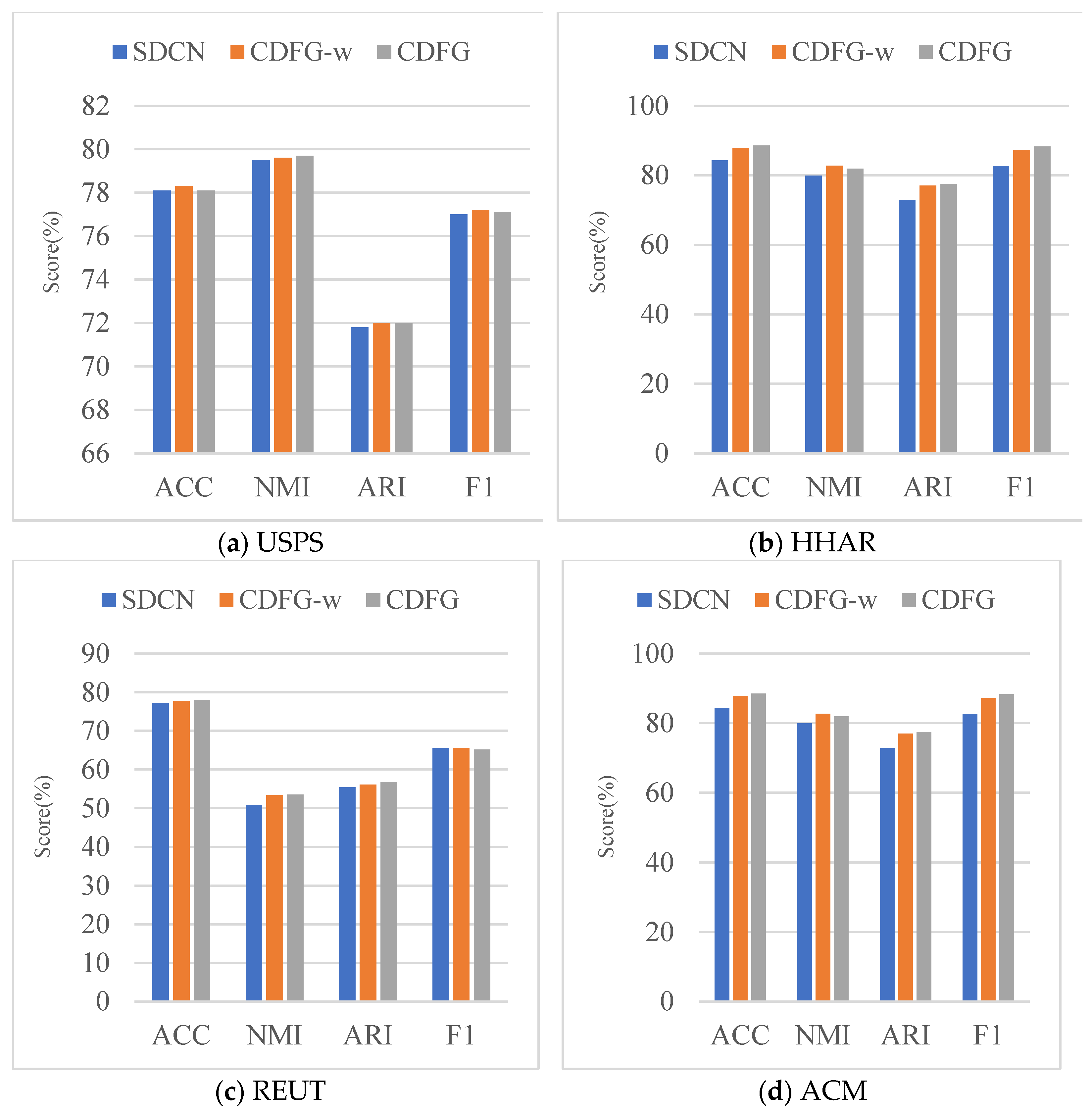
We conduct an ablation study to evaluate the effectiveness of the GAT module and the feature fusion module. The results are reported in
Figure 2.
Analysis of the GAT module. From
Figure 2, we can see that CDFG-w has a 0.1% to 4.6% improvement over the SDCN method, which shows the effectiveness of the graph attention network module. For non-graph datasets, the CDFG-w method performs better on HHAR than the other two non-graph datasets. For graph datasets, the CDFG-w method performs better on DBLP and CITE. The improvement is greater for networks with longer average path lengths and network diameters and smaller clustering coefficients, i.e., HHAR, DBLP, and CITE, which means that the graph attention layer considering high-order neighborhood information is more effective for this type of network.
Analysis of the feature fusion module. The CDFG has a 0.1% to 4.3% improvement over the CDFG-w method, which demonstrates the effectiveness of the feature fusion module. We can find that CDFG method performs better on graph datasets than non-graph datasets. For graph datasets, the CDFG method performs better on DBLP than on CITE. Similarly, the feature fusion module is more effective for networks with long average path length and network diameter and a small clustering coefficient. In addition, the feature fusion module improves the dataset with actual graph structure to a greater extent than the KNN graph because the dataset with actual graph structure reflects the characteristics of the data more accurately. Moreover, the model learns better after further enhancement of the features.
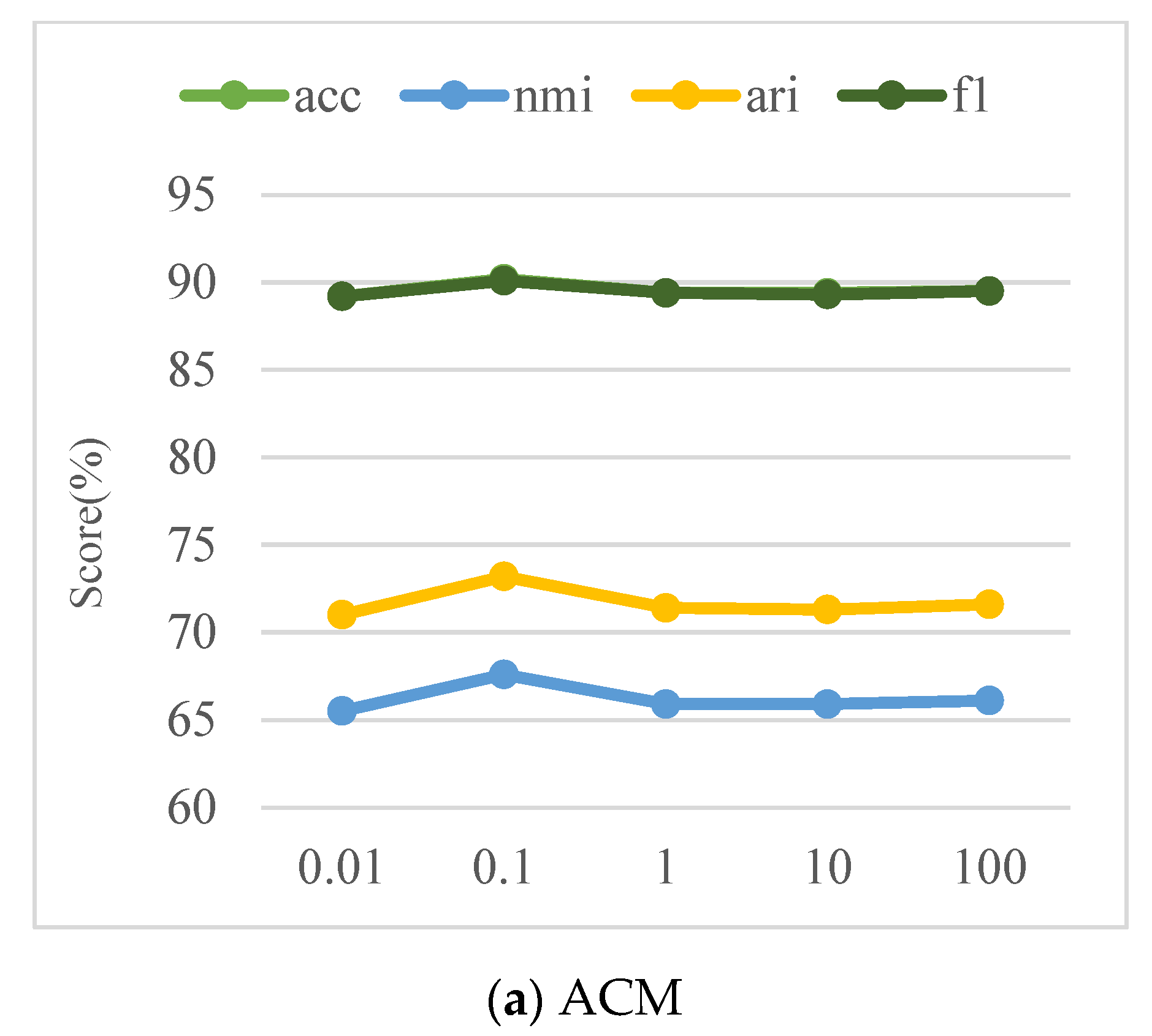
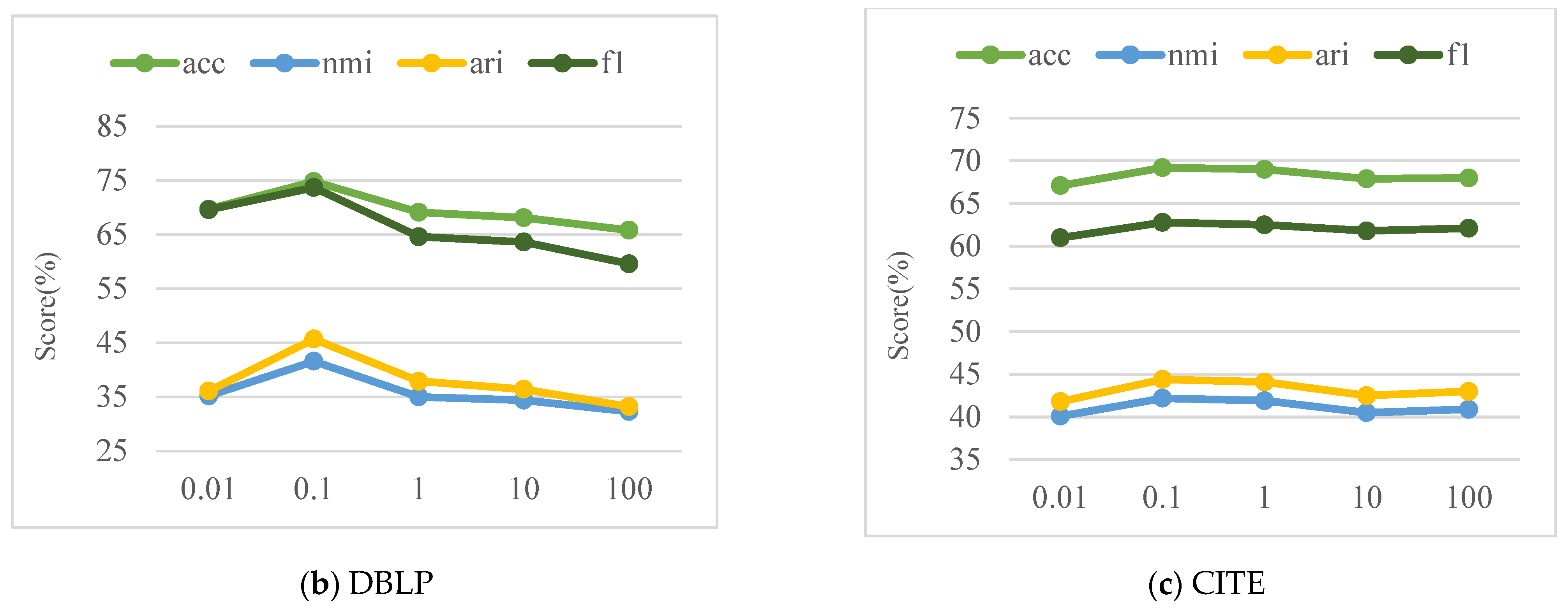
4.5. Parameter α Sensitivity Analysis
We conduct parameter sensitivity analysis of
in the loss function, which is an important parameter for balancing the clustering loss and other losses. To evaluate the effect of parameter
on model performance, the CDFG model is experimented with three graph datasets, including ACM, DBLP, and CITE, by setting
with fixed
. We do not discuss
here because the CDFG method is insensitive to
. We ran our method 10 times independently for each dataset and report the average results. The results of each metric are shown in
Figure 3.
From
Figure 3, we can observe that the parameter
has a certain influence on the clustering effect, and all three datasets reach the optimal value when
. For ACM and CITE, the trend of changes is gentler with the parameter
. However, for DBLP, the variation is more significant compared to ACM and CITE. From the viewpoint of network characteristics, networks with longer average path length and network diameter and smaller clustering coefficient are more sensitive to the change of parameter
.
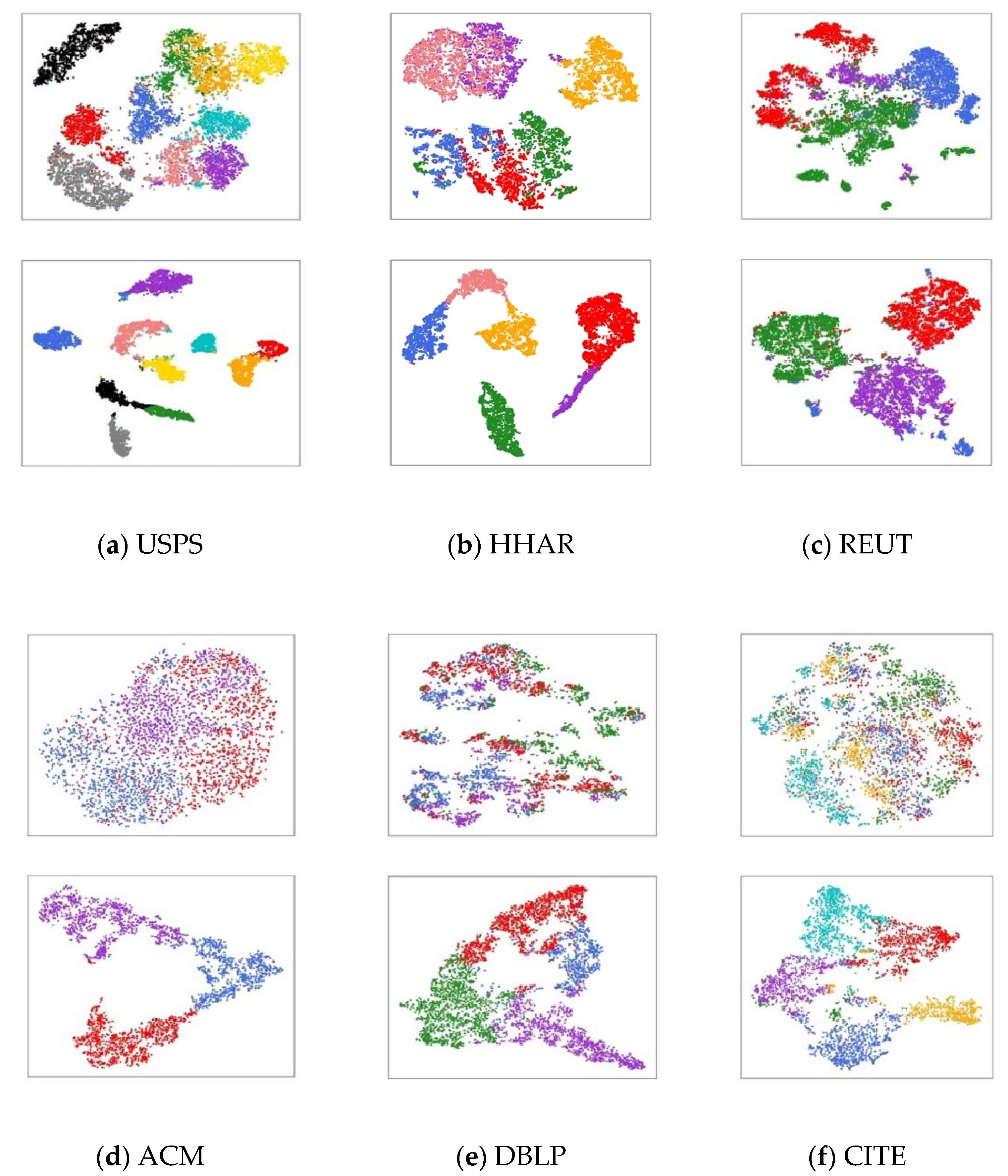
4.6. Network Visualisation
In order to verify the validity of the model more intuitively, we conduct an experiment visualizing the clustering results. For the original data, we use PCA firstly to reduce the dimension as the embedding representation obtained by CDFG, and use the t-SNE [
32] method for 2D visualization. For the learned embedding results, we directly visualize the data samples in 2D space by using the t-SNE method. The visualization results are shown in
Figure 4. The data points of the same color indicate the same category. The clearer the boundary between clusters composed of sample points of different colors, the better the clustering results.
The visualization results show that the original data distribution is more scattered, and the boundary is more confusing, while after the representation learning of the model, the same category is more aggregated, and the boundary between categories is clearer, which can verify the validity of the CDFG.
5. Conclusions
In this paper, we propose a community detection model fusing the graph attention layer and the autoencoder. The innovation of the model is that it fuses the autoencoder and the graph attention network with high-order neighborhood information for the first time. In addition, the feature fusion module is designed to achieve secondary fusion. The graph attention layer learns structural features better by considering the importance of neighborhood information. Adding high-order neighborhood information is more robust and effective for networks with longer mean paths and network diameters. The autoencoder learns the data characteristics, and a balance parameter fuses the two parts. The feature fusion module makes a secondary fusion of structural and attribute features. The experimental results show that the proposed model performs better on network datasets with longer mean paths and network diameters and smaller clustering coefficients. Compared with various state-of-the-art methods, CDFG has better performance for community detection.
This is because the use of the graph attention network calculates the influence weight of the neighborhood node on the target node through the attention mechanism, taking into account the difference of the influence of different neighborhood nodes. At the same time, high-order neighborhood information is added to the graph attention layer. The final node representation contains more information. On the other hand, the feature fusion module further fuses the structure information and the attribute information, and enhances the feature.
Currently, the model only supports non-overlapping community detection and it is a research direction to make model support overlapping community detection in the future. How to improve the efficiency of the algorithm while keeping the excellent performance of the model is also worth studying.
Author Contributions
Conceptualization, R.G. and W.W.; methodology, R.G. and J.Z.; software, Q.B.; validation, Q.B. and X.C.; formal analysis, W.W.; investigation, R.G. and J.Z.; resources, R.G. and J.Z.; data curation, W.W.; writing—original draft preparation, Q.B.; writing—review and editing, W.W.; visualization, X.C.; supervision, R.G.; project administration, W.W.; funding acquisition, R.G. All authors have read and agreed to the published version of the manuscript.
Funding
This research was funded by the People’s Livelihood Project of the Key R&D Program of Hebei Province (20375701D) and the Central Guidance on Local Science and Technology Development Fund of Hebei Province (226Z1808G).
Data Availability Statement
Conflicts of Interest
The authors declare no conflict of interest.
References
- Bo, Y.; Liu, D.; Liu, J. Discovering Communities from Social Networks: Methodologies and Applications. In Handbook of Social Network Technologies & Applications; Springer: Berlin/Heidelberg, Germany, 2010; pp. 331–346. [Google Scholar]
- Satuluri, V.; Wu, Y.; Zheng, X.; Qian, Y.; Wichers, B.; Dai, Q.; Tang, G.M.; Jiang, J.; Lin, J. SimClusters: Community-Based Rep-resentations for Heterogeneous Recommendations at Twitter. In Proceedings of the 26th ACM SIGKDD Conference on Knowledge Discovery and Data Mining, Virtual Event, CA, USA, 6–10 July 2020; ACM: New York, NY, USA; pp. 3183–3193. [Google Scholar]
- Keyvanpour, M.R.; Shirzad, M.B.; Ghaderi, M. AD-C: A new node anomaly detection based on community detection in social networks. Int. J. Electron. Bus. 2020, 15, 199. [Google Scholar] [CrossRef]
- Saidi, F.; Trabelsi, Z.; Ghazela, H.B. A novel approach for terrorist sub-communities detection based on constrained evidential clustering. In Proceedings of the 12th International Conference on Research Challenges in Information Science (RCIS), Nantes, France, 29–31 May 2018. [Google Scholar]
- Amini, A.A.; Chen, A.; Bickel, P.J.; Levina, E. Pseudo-likelihood methods for community detection in large sparse networks. Ann. Stats 2013, 41, 2097–2122. [Google Scholar] [CrossRef]
- Girvan, M.; Newman, M.E. Community structure in social and biological networks. Proc. Natl. Acad. Sci. USA 2002, 99, 7821–7826. [Google Scholar] [CrossRef] [PubMed]
- Chunaev, P. Community detection in node-attributed social networks: A survey. Comput. Sci. Rev. 2020, 37, 100286. [Google Scholar] [CrossRef]
- Wu, Z.; Pan, S.; Chen, F.; Long, G.; Zhang, C.; Yu, P.S. A Comprehensive Survey on Graph Neural Networks. IEEE Trans. Neural Netw. Learn. Syst. 2021, 32, 4–24. [Google Scholar] [CrossRef] [PubMed]
- Cao, S.; Lu, W.; Xu, Q. Deep neural networks for learning graph representations. Proc. AAAI Conf. Artif. Intell. 2016, 30, 1145–1152. [Google Scholar] [CrossRef]
- Velikovi, P.; Cucurull, G.; Casanova, A.; Remero, A.; Lio, P.; Bengio, Y. Graph Attention Networks. arXiv 2018, arXiv:1710.10903. [Google Scholar]
- Su, X.; Xue, S.; Liu, F.; Wu, J.; Zhou, C.; Hu, W.; Paris, C.; Nepal, S.; Jin, D.; Sheng, Q.Z. A Comprehensive Survey on Community Detection with Deep Learning. IEEE Trans. Neural Netw. Learn. Syst. 2021, 1–21. [Google Scholar] [CrossRef]
- Lecun, Y.; Bengio, Y.; Hinton, G. Deep learning. Nature 2015, 521, 436–444. [Google Scholar] [CrossRef]
- Kip, F.T.N.; Welling, M. Semi-Supervised Classification with Graph Convolutional Networks. arXiv 2016, arXiv:1609.02907. [Google Scholar]
- Kip, F.T.N.; Welling, M. Variational Graph Autoencoders. arXiv 2016, arXiv:1611.07308. [Google Scholar]
- Wang, C.; Pan, S.; Hu, R.; Long, G.; Jiang, J.; Zhang, C. Attributed Graph Clustering: A Deep Attentional Embedding Approach. arXiv 2019, arXiv:1906.06532. [Google Scholar]
- Wang, C.; Pan, S.; Yu Celina, P.; Hu, R.; Long, G.; Zhang, C. Deep neighbor-aware embedding for node clustering in attributed graphs. Pattern Recognit. 2022, 122, 108230. [Google Scholar] [CrossRef]
- Pan, S.; Hu, R.; Fung, S.F.; Long, G.; Jiang, J.; Zhang, C. Learning Graph Embedding with Adversarial Training Methods. IEEE Trans. Cybern. 2020, 50, 2475–2487. [Google Scholar] [CrossRef]
- Bo, D.; Wang, X.; Shi, C.; Zhu, M.; Lu, E.; Cui, P. Structural Deep Clustering Network. In Proceedings of the Web Conference (WWW 20), Taipei, Taiwan, 20–24 April 2020; pp. 1400–1410. [Google Scholar]
- Tu, W.; Zhou, S.; Liu, X.; Guo, X.; Cai, Z.; Zhu, E.; Cheng, J. Deep Fusion Clustering Network. In Proceedings of the AAAI Conference on Artificial Intelligence, Virtually, 2–9 February 2021; pp. 1–10. [Google Scholar]
- Kim, D.; Oh, A. How to Find Your Friendly Neighborhood: Graph Attention Design with Self-Supervision. arXiv 2021, arXiv:2204.04879. [Google Scholar]
- Liao, H.; Hu, J.; Li, T.; Du, S.; Peng, B. Deep linear graph attention model for attributed graph clustering. Knowl. Based Syst. 2022, 246, 108665. [Google Scholar] [CrossRef]
- Dong, Y.; Wang, Z.; Du, J.; Fang, W.; Li, L. Attention-based hierarchical denoised deep clustering network. World Wide Web 2022, prepublish. [Google Scholar] [CrossRef]
- Zhao, Q.; Ma, H.; Guo, L.; Li, Z. Hierarchical attention network for attributed community detection of joint representation. Neural Comput. Appl. 2022, prepublish. [Google Scholar] [CrossRef]
- Xie, J.; Girshick, R.; Farhadi, A. Unsupervised Deep Embedding for Clustering Analysis. In Proceedings of the 33rd International Conference on Machine Learning, New York, NY, USA, 19–24 June 2016; pp. 478–487. [Google Scholar]
- Guo, X.; Gao, L.; Liu, X.; Yin, J. Improved Deep Embedded Clustering with Local Structure Preservation. In Proceedings of the Twenty-Sixth International Joint Conference on Artificial Intelligence (IJCAI-17), Melbourne, Australia, 19–25 August 2017; pp. 1753–1759. [Google Scholar]
- Huang, X.; Hu, Z.; Lin, L. Deep clustering based on embedded auto-encoder. Soft Comput. 2021. prepublish. [Google Scholar] [CrossRef]
- Peng, Z.; Jia, Y.; Liu, H.; Hou, J.; Zhang, Q. Maximum Entropy Subspace Clustering Network. IEEE Trans. Circuits Syst. Video Technol. 2022, 32, 2199–2210. [Google Scholar] [CrossRef]
- Hinton, G.E.; Salakhutdinov, R.R. Reducing the Dimensionality of Data with Neural Networks. Science 2006, 313, 504–507. [Google Scholar] [CrossRef] [PubMed]
- Cui, Y.L.; Matan, O.; Boser, B.; Denker, J.S.; Henderson, D.; Howard, R.E.; Hubbard, W.; Jacket, L.D.; Baird, H.S. Handwritten zip code recognition with multilayer networks. In Proceedings of the International Conference on Pattern Recognition, Atlantic City, NJ, USA, 16–21 June 1990; IEEE: Piscataway, NJ, USA. [Google Scholar]
- Stisen, A.; Blunck, H.; Bhattacharya, S.; Prentow, T.S.; Kjargaard, M.B.; Den, A.K.; Sonne, T.; Jensen, M.M. Smart devices are different: Assessing and mitigating mobile sensing heterogeneities for activity recognition. In Proceedings of the Acm Conference on Embedded Networked Sensor Systems, Seoul, Korea, 1–4 November 2015; ACM: New York, NY, USA, 2015. [Google Scholar]
- Lewis, D.D.; Yang, Y.; Rose, T.G.; Li, F. RCV1: A New Benchmark Collection for Text Categorization Research. J. Mach. Learn. Res. 2004, 5, 361–397. [Google Scholar]
- van der Maaten, L.; Hinton, G. Visualizing data using t-sne. J. Mach. Learn. Res. 2008, 9, 2579–2605. [Google Scholar]
| Publisher’s Note: MDPI stays neutral with regard to jurisdictional claims in published maps and institutional affiliations. |
© 2022 by the authors. Licensee MDPI, Basel, Switzerland. This article is an open access article distributed under the terms and conditions of the Creative Commons Attribution (CC BY) license (https://creativecommons.org/licenses/by/4.0/).


